Galaxy systems in the optical and infrared

Abstract

In these three lectures a review is provided of the properties of galaxy systems as determined from optical and infrared measurements. Covered topics are: clusters identification, global cluster properties and their scaling relations, cluster internal structure and dynamics, and properties of cluster galaxy populations.

1 Identification, global properties, and scaling relations

1.1 Identification

Historical identifications of clusters of nebulæ  date back to the late years of the XVIII century [1]. The first modern method of galaxy clusters identification and classification was implemented by Abell [2] in 1958. Abell worked out apparent overdensities of galaxies in the sky by eye inspection of photographic plates of the Palomar Observatory Sky Survey. He used the apparent magnitudes of galaxies to determine approximate cluster distances which he then used to convert apparent sizes to physical sizes. Abell characterized clusters by their richness, i.e. the number of galaxies in the 2 mag range $m_{3}$ to $m_{3}+2$ in a circle of radius 2.1 Mpc, corrected for the contamination by fore- and back-ground galaxies. We now refer to this radius as the ’Abell radius’; it is still widely used as a typical cluster size since it is rather close to the virial radius, $r_{200}$, of a massive cluster with a velocity dispersion $\sigma_{v}\simeq 900$ km s^-1.

Abell’s catalog contained 2712 clusters, later extended to the southern hemisphere [3] to a total of 4073 clusters. Thanks to Abell’s early work, galaxy clusters started to be studied as a class and not only as individual objects. Abell’s catalog has formed the basis of the largest galaxy cluster-specific spectroscopic survey completed so far, the ESO Nearby Abell Cluster Survey (ENACS [4, 5]).

Abell’s cluster sample suffers however from two main problems, incompleteness and contamination by projection effects [6, 4], although these problems are less severe than it is usually stated [7]. Incompleteness and contamination are crucial issues, in particular for cosmological studies, like e.g. the determination of the cluster mass function and its redshift evolution (see Sect. 1.4). Ideally one would like to have a cluster sample with zero contamination and 100% completeness. Since this is not possible, it becomes essential that contamination and incompleteness can be precisely estimated, so that the statistical sample can be corrected for. A precise estimate of the contamination and incompleteness of a cluster catalog can be obtained by applying the cluster identification technique to mock galaxy samples extracted from cosmological numerical simulations. This of course requires the identification technique to be exactly reproducible, and Abell’s eye is not.

The main difference of today’s clusters identification techniques with respect to Abell’s is that they are both automated and objective. Automatization requires either that photographic plates be digitized, or that data are digital in origin, coming from CCD cameras [8]. Besides automatization and objectiveness, modern clusters identification techniques also have a well-understood selection function and impose minimal a priori constraints on the properties of the systems to be identified [9]. These characteristics are now common to many cluster identification methods which have been developed over the years. Among these, some have been specifically developed to be used on photometric galaxy samples and some on spectroscopic galaxy samples.

Among the methods applicable to samples of galaxies without redshift information, the most used is the Matched Filter (MF hereafter [10]). In summary, the method works as follows. The spatial and luminosity distribution of observed galaxies in a given field is modeled as the sum of two contributions, one from the field, another from the cluster

$$D(R,m)=b(m)+N_{c}N(R)\phi(m).$$ (1)

The term $b(m)$ represents the background galaxy counts at a given magnitude, $m$. The cluster term is itself the product of three factors. $N(R)$ is the projected radial profile of the cluster galaxies as a function of the projected radial distance from the cluster center, $R$, $\phi(m)$ is the differential cluster luminosity function (LF hereafter; see Sect. 1.2), and $N_{c}$ is a measure of the cluster richness, or multiplicity. Both $N(R)$ and $\phi(m)$ can depend on free parameters, typically a characteristic length scale and a characteristic magnitude. The best-fit free parameters are found through a Maximum Likelihood procedure aimed at minimizing the difference between the observed galaxy distribution, $D(R,m)$, and the model. Clusters are identified by searching for local maxima within a moving box of given size centered on each pixel of the filtered galaxy map array (or at each galaxy position [11]). If the central pixel in the box is a local maximum, and if the maximum exceeds a given threshold (which depends on the background noise), a candidate cluster is registered. An estimate of the cluster redshift results from assuming a universal value for the absolute characteristic magnitude of the LF. Several variants of the MF method have been proposed [11, 12, 13].

Among the methods applicable to samples of galaxies with redshift information, by far the most used is the friends-of-friends percolation algorithm (FoF hereafter, see [14, 15]). This method links together all galaxies within a chosen linking volume centered on each galaxy. At variance with Abell’s method, galaxy systems are identified within a physical overdensity, not within a physical (fixed) size. Since the density of galaxies in a flux-limited survey depends on redshift, the linking volume is also scaled with redshift. In practice, specifying the linking volume is equivalent to specifying two linking lengths, one in the plane of the sky, another along the redshift direction. Different works have adopted different linking lengths, and different scalings with the galaxy density (compare, e.g., [14] to [16]). The linking lengths have been chosen using a priori knowledge of the physical characteristics of the galaxy systems one is looking for [17], or by minimizing the differences between the recovered and intrinsic properties of systems identified in a mock galaxy sample [18].

While originally conceived to work on imaging surveys, in its modified versions the MF method can also be applied to spectroscopic surveys [11, 13]. Symmetrically, when the redshift information is not available, it is still possible to adopt the FoF method, using photometric, rather than spectroscopic, redshifts [19]. Nevertheless, applications of the MF (respectively, FoF) method have so far mostly concerned data from photometric (respectively, spectroscopic) surveys.

The MF algorithm has been applied to data from the ESO Imaging Survey [20, 12], the Sloan Digital Sky Survey (SDSS [21]), the 2 Micron All Sky Survey (2MASS [22]), and several other surveys [23, 24, 25, 26, 19]. Clusters in the resulting catalogs are detected out to $z\sim 1$ and beyond, and down to masses $\sim 10^{14}\,M_{\odot}$, depending on the depth of the photometric survey. Spectroscopic follow-ups show the photometrically identified high-$z$ cluster candidates to be real [27, 28]. Comparison to mock catalogs show that completeness can reach $\sim 100$% for $\sim 10^{14}\,M_{\odot}$ mass clusters out to intermediate-$z$, and $\sim 50$% for very massive clusters ($\sim 10^{15}\,M_{\odot}$) out to $z\sim 1.5$ [19, 13]. In comparison to X-ray cluster surveys, these optical cluster surveys have been able to detect lower-mass clusters [24, 29] and clusters with an X-ray luminosity below what expected given their mass (see, e.g., [30, 31, 32]). Less than 10% of X-ray detected clusters with $z\leq 0.5$ are missed in these optical cluster surveys [33].

The FoF method has been applied to many spectroscopic surveys, e.g. the Center for Astrophysics Redshift Survey [15, 16, 34], the Southern Sky Redshift Survey [35], the Las Campanas Redshift Survey [36], the ESO Slice Project survey [37], and, more recently, the SDSS, the Two Degree Field Galaxy Redshift Survey (2dFGRS), and the 2-Micron All Sky Redshift Survey (2MRS) [17, 38, 18, 39, 40, 41]. The resulting catalogs list up to several thousands of galaxy systems. Most of them are small galaxy groups, with median velocity dispersion and mass $\sigma_{v}\sim 200$ km s^-1, $M\sim 10^{13}\,M_{\odot}$. Clearly, identification in 3-d space (spatial coordinates and redshifts) allows to detect lower-mass systems than identification in projected spatial distribution only. On the other hand, the higher depth of photometric surveys allows the detection of (rather massive) clusters out to higher-$z$.

Several other cluster identification methods have been implemented. Some methods start with a FoF identification, then provide a first estimate of the mass of the identified system, and use this estimate to determine which galaxies belong to the group, in an iterative way [42, 43, 44]. These variants of the FoF method try to minimize contamination by galaxies that are close in redshift but not in real space (interlopers). This is crucial when the contamination risk is high, like in medium- or high-$z$ samples. An application of this technique to the Canadian Network for Observational Cosmology (CNOC) $2^{nd}$ survey has produced a catalog of $\sim 200$ galaxy groups at a median $z=0.33$ [42].

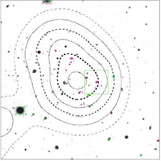
Figure 1: Color composite image of a cluster identified with the CRS technique [46]. The cluster is located at an estimated redshift of 0.952. Red-sequence galaxies are displayed with a reddish color in the figure, and red-sequence galaxy isodensity contours are displayed. The rectangle identify the BCG. The image size is $15^{\prime}\times 15^{\prime}$, i.e. $\sim 7\times 7$ Mpc at the cluster estimated distance. Note how the galaxy colors are helpful in identifying the cluster against the background.

The Cluster Red Sequence (CRS hereafter [45]) method is based on the observation that all rich clusters, at all redshifts up to $z\sim 1$, have a more or less well defined red sequence of galaxies in a color–magnitude diagram, where the color is defined by two photometric bands bracketing the 4000 Å  break feature of galaxy spectra. Since the 4000 Å  break is redshifted into different observational bands depending on the galaxy $z$, with a suitable set of filters it is possible to define color-cuts to select galaxies at a redshift close to the cluster mean redshift. By comparison with spectrophotometric models, the CRS method also provides estimates of the mean redshifts of the detected clusters, with an accuracy superior to that reached by the MF method [45]. Roughly speaking, the method consists in slicing a given galaxy catalog in color, computing the galaxy surface density of that slice, and identifying significant overdensities. An example of a cluster detected with this technique [46] at an estimated redshift $z\sim 1$ is shown in Fig. 1.

The CRS method has been first tested on the CNOC-2 data-set, for which spectroscopy is available, using only two-band photometry. In practice, this is a comparison of the photometric CRS vs. the spectroscopic FoF methods. The fraction of clusters detected with the CRS and undetected with the FoF method, i.e. the fraction of false positive CRS detections, is only 1/23 out to $z=0.5$, and the CRS photometric $z$-estimates are accurate to $\Delta z=0.03$. Given that many of the identified systems are groups rather than rich clusters, the performance of the CRS method is remarkable. Application of this method to mock data-sets extracted from the Millennium simulation has shown that projection effects are of relatively minor importance in the great majority of the identified systems (80 to 90%, depending on $z$) [47].

The CRS method has been applied to photometric data obtained in two wavebands with large format mosaic cameras at CFHT and CTIO. The resulting catalog (the Red-sequence Cluster Survey, see [46, 48]) contains almost 1000 cluster candidates among which more than a hundred at $z\sim 1$, some of which have been spectroscopically confirmed [49, 46].

The CRS method has been applied to infrared (IR hereafter) data obtained with the IRAC camera onboard Spitzer [50, 51]. At higher $z$ the 4000 Å  break is progressively shifted towards the IR, hence deep IR observations are needed to detect cluster red-sequences at $z>1$. Hundreds of candidate clusters out to an estimated redshift $z=1.85$ have been found so far by this method using data from Spitzer surveys, of which more than one hundred above $z=1$ [50, 51]. Other spectral features than the 4000 Å  break can be used to define IR color cuts aimed at reducing the field galaxy contamination, e.g. the $\simeq 1.6\,\mu$m peak in the flux distribution of stellar populations [52]. Based on this spectral feature $z>1$ clusters can be selected by using two Spitzer IRAC bands (3.6 and 4.5 $\mu$m) which will still be in operation in the Spitzer postcryogenic era. Recently, data from the Japanese IR satellite AKARI have been used to detect candidate clusters at $0.9<z<1.7$ by exploiting both the 4000 Å  break and the $1.6\,\mu$m peak features [53].

Another cluster identification method that relies upon the existence of a red sequence for cluster galaxies, is maxBCG [21, 9]. The maxBCG method also relies on the location of the brigthtest cluster galaxy (BCG) near the cluster center. Application of this method to the SDSS data [54] has provided a catalog of 13,823 clusters with $\sigma_{v}>400$ km s^-1, out to $z=0.3$, with photometric $z$ estimates accurate to $\Delta z\simeq 0.01$. Comparison with a cluster catalog constructed by applying the MF method on the same data-set has shown that $\sim 80$% of the systems are identified by both the maxBCG and the MF method [21]. The imperfect matching may be due to the presence of substructures (see Sect. 2.5) identified as distinct clusters by the maxBCG method, and to the presence of false positives in both catalogs. Comparison with mock catalogs indicates the maxBCG cluster catalog is 90% pure and 85% complete for clusters with masses $\geq 10^{14}\,M_{\odot}$.

Relying upon the existence of a red sequence for cluster galaxies has certainly proven to be a very effective way of selecting galaxy clusters. On the other hand, unrelaxed, low-mass galaxy clusters in which this sequence is not established yet, or at least not very prominent [24], may be missed by CRS methods and alike. This is particularly true at high $z$, since the fraction of early-type galaxies (ETGs in the following) decreases with $z$ (see Sect. 3.1) making the red sequence less and less prominent. For this reason, other cluster detection methods make use of multi-band photometry to allow a wider selection of galaxy spectral types, star-forming galaxies included. Typically, but not exclusively, this is done by defining photometric-$z$ through the comparison of the galaxy spectral energy distributions with model templates. The Cut and Enhance (CE) [55] and the C4 methods [56] have been developed to make full use of the SDSS 4-bands photometry.

At high $z$, IR photometry proves essential to identify galaxy cluster candidates. A clear demonstration of the potential of cluster searches conducted in the IR is the detection of a $z=1.41$ cluster [57]. This cluster has been identified in the Spitzer IRAC Shallow survey as an overdensity of IR-selected galaxies (see also [58, 50]). Each galaxy was assigned a photometric-redshift probability distribution, which was then used to weigh the density maps within overlapping redshift slices. A wavelet technique was adopted to smooth the density field, in which significant peaks were then looked for. The $z=1.41$ cluster is only the highest-$z$ confirmed detection among 335 galaxy cluster and group candidates (average mass $\sim 10^{14}\,M_{\odot}$) found with this technique in a 7.25 deg² region in the Spitzer IRAC Shallow survey [59, 50]. Over a hundred of the cluster candidates have a redshift above unity, with an estimated spurious detection rate of 10%. Twelve of the $z>1$ candidates have already been spectroscopically confirmed. Unfortunately, the photometry is not deep enough to identify clusters much beyond $z\approx 1.5$ [59].

IR-color selection is also useful to improve the efficiency of spectroscopic follow-ups of high-$z$ clusters identified in other wavebands, e.g. in X-rays [60, 61].

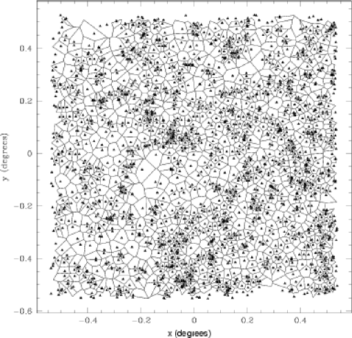
Figure 2: An example of Voronoi tesselation of a galaxy field. Each triangle represents a galaxy position on the plane of the sky [62].

A rather different method for the identification of galaxy systems is the Voronoi Galaxy Cluster Finder (VGCF [62]). In this method, the projected space is divided in cells according to the Voronoi tesselation technique, each cell containing a single point (i.e. a galaxy; see Fig. 2). The inverse of the cell area defines the local galaxy density. Clusters are defined as ensembles of adjacent cells with a density above a given threshold. The search for clusters is done in magnitude bins. The main advantages of this method is that it is nonparametric and as such it does not require a priori hypotheses on the cluster properties, such as cluster size, density profile, or shape. The VGCF method has been shown to be competitive with (or even better than) the MF method [63]. A comparison between the CE, MF, maxBCG, and VCGF methods has shown that at low redshifts ($z<0.4$) the CE is more complete, but pays the price of a higher rate of false detections ($\sim 30$%) as measured from Monte Carlo simulations [55].

If multicolor photometry is available, the VGCF method can be applied to subsamples selected in the color-magnitude diagram, thus reducing the field contamination by the same technique adopted in the CRS method [64]. This VGCF+CRS method has been used to detect clusters in fields previously observed by the Chandra X-ray satellite [65]. The optical detection fraction of X-ray-detected clusters was 46% vs. an X-ray detection fraction of optically-detected clusters of only 11%. While part of the optical detections may be spurious, the cluster detection threshold was clearly lower in the optical catalogs than in the X-ray catalogs. Galaxy-rich clusters without X-ray counterparts are also detected, suggesting the existence of a population of underluminous (perhaps not yet virialized) X-ray clusters (see, e.g., [30, 31, 32]). Sufficiently deep photometric data-sets allow the VGCF method to detect clusters as far as $z\sim 1$ and beyond [19].

With some modifications [66], the VGCF method has also been used on 3-d data-sets, such as the DEEP2 Galaxy Redshift Survey, resulting in a catalog of 105 galaxy systems with median $z=0.86$, and median $\sigma_{v}=480$ km s^-1 [67].

Eventually, when the data are too shallow to rely on galaxy number counts, it is possible to identify cluster candidates as positive surface-brightness fluctuations (SBF) in the background sky [68, 69]. An application of the SBF method to a drift-scan survey has produced a catalog of $\sim 1000$ cluster candidates at $z\leq 0.8$, the Las Campanas Distant Cluster Survey (LCDCS [68, 70]). At $z<0.3$, the catalog contains systems with masses typical of galaxy groups. This catalog has formed the basis for the ESO Distant Cluster Survey (EDisCS [71]), in which 20 LCDCS candidate clusters have been followed up spectroscopically with VLT/FORS2.

Going to the next step of the cosmic hierarchy, catalogs of clusters can be used to define superclusters [72]. Superclusters have been identified either by the FoF percolation technique [73, 74, 75, 76], or as overdensities in smoothed cluster-density fields [77, 78, 79]. Large-scale structure morphology has also been characterized statistically, without the need of defining superclusters, e.g. by the Genus statistics [80], or by the use of Minkowski functionals [81] and their combination (the Shapefinder statistic, see [82]).

1.2 Global properties: richness, luminosity, mass

In order for cluster catalogs to be useful in cosmological studies, they should also provide cluster mass estimates. Cluster masses can be estimated directly, by applying dynamical methods (virial theorem, Jeans equation, …) to the sample of cluster galaxies, if redshifts are available; by solving the hydrostatic equation for the X-ray emitting intra-cluster plasma; or by analyzing the effects of gravitational lensing on background galaxies in the cluster field. All these methods are very expensive in terms of telescope time, hence it is customary to use cheaper global cluster quantities that can serve as mass proxies. In optical cluster studies, the most used mass ($M$ hereafter) proxies are the cluster richness (or multiplicity), $N$, namely the number of galaxies contained in a cluster, and the cluster luminosity, $L$, both measured in a certain magnitude range and out to a certain radius from the cluster center.

$N$ and $L$ are evaluated by counting galaxies and, respectively, summing their luminosities, in a given region of space where we know the sample is uniformly complete down to a certain magnitude, $m_{c}$. If the sample suffers from incompleteness, a correction must be applied. Both $N$ and $L$ must then be corrected by subtracting the expected contamination by field galaxies (which can be estimated in a comparison empty field or from the number counts of general field galaxy surveys, see, e.g., [83]). In comparing the $N$ and $L$ estimates of clusters at different distances, the limiting magnitudes used must be accordingly scaled.

If one is looking for a mass proxy, the summed luminosity of the brightest galaxies could suffice. On the other hand, if what is needed is the total cluster luminosity, an extrapolation is required to account for the contribution of the faint galaxies with $m>m_{c}$. Such an extrapolation is done by fitting a suitable function to the observed magnitude distribution, and then integrating this function from $m_{c}$ to the magnitude of the faintest galaxies. By far, the most widely used function is the Schechter LF [84]

$$\phi(l)dl=\phi_{\star}\,(l/l_{\star})^{\alpha}\,\exp(-l/l_{\star})\,d(l/l_{\star}),$$ (2)

where $l$ is the galaxy luminosity, $l_{\star}$ and $\phi_{\star}$ are the characteristic luminosity and number density, respectively, and $\alpha$ is the faint-end power-law exponent. Galaxy luminosities are derived by converting galaxy apparent magnitudes into absolute magnitudes via knowledge of the cluster luminosity distance and of the Galactic extinction in the observational photometric band (see, e.g., [85]). In order to get an estimate of the total cluster luminosity within a given radius, e.g. the overdensity radius $r_{200}$, one must determine the luminosity density profile, Abel-invert it to obtain the 3-d profile (see eq. (10) in Sect. 2.1), and finally extrapolate it to the desired radius with a suitable fitting function (e.g. a projected ’NFW’ profile [87, 88]; see also Sect. 2).

By the same technique it is in principle possible to get an estimate of $N(<r_{200})$. However, extrapolation to fainter magnitudes is in this case dangerous, since faint galaxies largely outnumber bright galaxies, while their integrated contribution to the total luminosity is only marginal. A more robust estimate of a cluster richness is provided by the $B_{gc}$ parameter [89], the galaxy cluster center correlation amplitude. It is measured by counting galaxies in a fixed aperture around the cluster center, it requires an assumption about the shape of the correlation function and the LF, and it must be corrected for the field galaxy contamination. $B_{gc}$ is almost independent of the fixed aperture and chosen limiting magnitude [90].

The most classical direct method to determine $M$, the cluster mass, is by applying the virial theorem to the projected phase-space distribution of cluster galaxies (e.g. [86]). This method has been in use since the ’30s, when Zwicky and Smith [91, 92, 93] provided the first preliminary mass estimates of the Coma and Virgo clusters. Their studies marked the discovery of dark matter (DM hereafter; see, e.g. [1]). The virial theorem is obtained by integrating the equation of hydrostatic equilibrium for the galaxy distribution in the potential well of a cluster (the Jeans equation, see [86]). In terms of the observables the virial theorem can be expressed as follows,

$$M=3\pi\,P\,\sigma_{v}^{2}\,R_{h}/G,$$ (3)

where $G$ is the gravitational constant, $\sigma_{v}$ is the line-of-sight velocity dispersion of cluster galaxies, and $R_{h}$ is the harmonic mean radius of the projected spatial distribution of cluster galaxies,

$$R_{h}=\frac{1}{2}\frac{n(n-1)}{\sum_{i>j}\,R_{ij}^{-1}},$$ (4)

where $R_{ij}$ is the projected distance between two cluster galaxies, and $n$ is the number of cluster galaxies. The factor $3\pi$ corrects for projection effects [94, 96]. The factor $P$ is the surface pressure term [95, 96]. It is a correcting factor needed when the entire cluster is not included in the observed sample. It can be understood as follows. Suppose you have a galaxy orbiting a cluster with its apocenter at radius $a$ and you observe the cluster only out to the radius $r_{l}$, with $r_{l}<a$. Making the wrong assumption that the entire cluster has been observed corresponds to imposing a smaller apocenter to the galaxy, since $a$ cannot be larger than $r_{l}$ under this assumption. Given the galaxy velocity, the same orbital anisotropy, and the same cluster density profile, imposing a smaller value for the galaxy orbital apocenter corresponds to forcing a larger mass inside $r_{l}$. The correction factor can be evaluated as follows:

$$P=1-4\pi r_{l}^{3}\frac{\rho(r_{l})}{\int_{0}^{r_{l}}4\pi x^{2}\rho dx}\,\frac{\sigma_{r}^{2}(r_{l})}{\sigma^{2}(<r_{l})},$$ (5)

where $r_{l}$ is the limiting observational radius, $\rho(r)$ is the tracer mass density distribution, $\sigma_{r}$ is the radial component of the velocity dispersion, and $\sigma(<r_{l})$ is the integrated velocity dispersion within $r_{l}$ [96]. Knowledge of $\rho(r)$ and of the galaxy velocity anisotropy profile is formally needed in order to solve for $P$; in practice one uses theoretical prejudice in order to make reasonable assumptions for these profiles. The resulting $P$ estimate is therefore only an approximation, but this is preferable to no correction at all, since the correction factor is systematic, $P<1$ (typically, $P\simeq 0.8$–0.9 for a typical cluster observed out to $r_{l}\simeq 2$ Mpc [97]).

Since one is using the velocity and spatial distribution of cluster galaxies in eqs. (3,4), the resulting $M$ estimate will only be correct if the galaxies are distributed like the mass [95, 98]. Given that different galaxy populations are distributed differently in projected phase-space (see, e.g., [99]), the choice of the tracer may change the $M$ estimate rather substantially. Analysis of the mass profiles of galaxy clusters have shown that the distribution of ETGs and red-sequence galaxies is similar to that of the cluster mass (see Sect. 2.2), hence they are to be preferred over late-type, star-forming (blue) galaxies as tracers of the potential when using the virial theorem to determine the cluster mass. Virial masses estimated using late-type (emission-line) galaxies can be 50% higher than those derived from ETGs [100].

How reliable are the cluster masses derived by applying the virial theorem to cluster galaxies? An analysis of clusters extracted from cosmological numerical simulations has shown that their masses are only 10% overestimated by application of the virial theorem to samples of $n\geq 60$ particles (galaxies) [97]. Part of the overestimation is caused by the presence of interlopers, part by the presence of subclustering. Selecting only ETGs or only relaxed clusters reduces the bias in the mass estimate. Since much of the problem lies in the estimate of $R_{h}$, an alternative mass estimate based on $\sigma_{v}$ only can be a viable alternative to the virial mass estimate [101, 97].

Recent analyses of medium-distant clusters (CNOC, EDisCS) have shown that virial mass estimates based on cluster galaxies are entirely consistent with mass estimates based on gravitational lensing and/or on intra-cluster gas X-ray emission [102, 103], thus confirming the consistency found on local cluster samples [96, 104]. Other analyses have found that virial mass estimates are generally higher than the mass estimates based on X-ray emission [105, 106, 107, 108, 109, 110]. In general, the largest discrepancies between different mass estimates are found for dynamically unrelaxed clusters [108, 110, 111, 112].

An indirect confirmation of the reliability of virial mass estimates has come from the comparison of the values of cosmological parameters obtained using these mass estimates, with the values obtained by the Wilkinson Microwave Anisotropy Probe (WMAP [109, 113]).

1.3 Scaling relations

For a $M$-proxy to be effective, it is important to know precisely its scaling relation with the cluster mass, as well as the intrinsic scatter in this relation (see, e.g. [114]). The smaller this scatter, the better is the mass–proxy relation constrained. Moreover, it is important to know how scaling relations evolve with redshift. In fact, scaling relations are generally determined locally, on the best observational samples, yet they have to be applied over a wide redshift range in order to improve the constraints on cosmological parameters.

On the cluster scale, both $N$ and $L$ have been shown to be $M$ estimators of similar or even better accuracy than $L_{X}$ [89, 32, 115, 90]. The typical accuracy with which a cluster $M$ (within a given overdensity) can be predicted by $N$ or $L$ is $\sim 30-40$% [116, 117, 89, 118, 119, 56, 32, 90]. At least half of the observed scatter in the $M-N$ and $M-L$ relations appears to be intrinsic [90]. The scatter appears to increase at lower masses, although it is unclear how much of this increase is due to observational uncertainties and how much it is due to an intrinsic larger variance of the properties of low-mass galaxy systems [120]. The scatter decreases when irregular and substructured clusters are removed from the sample [121, 56].

The $M-N$ and $M-L$ relations are almost linear on the cluster scale, but not quite so, and most studies (with some notable exceptions [21, 22]) indicate a mild [122, 123, 116, 118, 119, 124, 32, 125, 90] or very mild [120, 54, 126] increase of the $M/L$ and $M/N$ ratio with cluster mass, $M/L\propto M^{a}$ with $a\simeq 0.2\pm 0.1$. The $M/L$ ratio is not however well described by a simple power-law from the cluster to the group mass scale. It steepens considerably for masses below $\simeq 3\times 10^{13}\,M_{\odot}$ reaching a minimum at $\sim 10^{12}\,M_{\odot}$ [116, 127, 128, 129] (see Fig. 3). The non-linearity of the $M-L$ relation at low masses is however of little concern for most cosmological studies based on cluster number density, since the completeness required by these studies is generally achievable only at the high-$M$ end, at least at high-$z$.

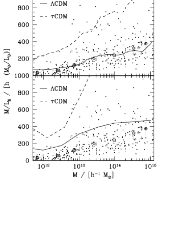
Figure 3: Observed $M/L$ ratio for clusters and groups (dots) and their median values (circles) with 90% confidence levels error bars, are compared with theoretical predictions from two semi-analytical models (upper panel: [130], lower panel: [131]). From [116].

The $M/L$ variation with $M$ in galaxy systems is well fit by the theoretical predictions of semi-analytical models (e.g. [130]; see Fig. 3) in which the efficiency of galaxy formation is inhibited by the reheating of cool gas on small-mass scales, and by the long cooling times of hot gas on large-mass scales (see, e.g. [127].) Other models that could produce the observed $M/L$ variation require galaxy merging and/or destruction to occur with different efficiency in galaxy systems of different mass. These mechanisms seem however to be ruled out by the similar shape of the LFs of clusters with different masses [126], and by the lack of any significant evolution of the cluster $N-M$ relation up to $z\sim 1$ [132, 133, 48, 134].

In order to understand the possible biases involved in converting a given proxy into an $M$ estimate, it is useful to compare scaling relations involving different proxies, or, equivalently, to determine the relations between them. In particular, it is interesting to compare optical and X-ray properties of galaxy clusters.

In the comparison of X-ray and optical properties of galaxy clusters, two anomalies emerge: (i) there is a population of optically selected clusters with too low an X-ray luminosity, $L_{X}$, for their $\sigma_{v}$ or optical richness (see Fig. 4; [30, 31, 135, 136, 65, 137, 32]), and (ii) there is a population of X-ray bright galaxy groups with too small a $\sigma_{v}$ for their X-ray temperature or luminosity [138, 139, 140].

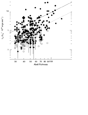
Figure 4: The relation between X-ray luminosity and richness for a sample of nearby optically-identified clusters. Filled circles are detections, open symbols are upper limits in X-ray luminosity (i.e. optically identified clusters undetected in X-ray). The solid (dotted) line is the relation that fits the data excluding (including) the non-detections. From [145].

The X-ray underluminous clusters appear anomalous only with respect to the $L_{X}-N$ relation established for X-ray-selected cluster samples. As a matter of fact, low-mass X-ray selected clusters do follow the same scaling relations established for clusters of higher masses [141]. But X-ray selection excludes low-$L_{X}$, high-$N$ clusters from the sample, leading to an $L_{X}-N$ relation that is biased high relative to the true underlying relation [24, 142, 143]. The true $L_{X}-N$ relation is characterized by a large dispersion of the $L_{X}$ values at given $N$. This can be partly explained by systematic errors in both the X-ray and optical estimates (see, e.g., [144]). However, part of the dispersion may be intrinsic and related to different properties of the X-ray underluminous clusters relative to the normal X-ray emitting cluster population. X-ray underluminous clusters appear in fact more irregular [145], and the properties of their galaxies are reminiscent of those of infalling field galaxies [32]. In other words, the X-ray underluminous clusters look like unvirialized systems.

While X-ray underluminous clusters may be systems at an early stage of their dynamical evolution, X-ray bright groups with abnormally small $\sigma_{v}$ may be systems at an advanced stage of their dynamical evolution. A possible way to reduce the group $\sigma_{v}$ is to slow down galaxies by the process of dynamical friction [146]. Although the characteristic time of this process is generally longer than a Hubble time for cluster galaxies, it is shorter than this for massive group galaxies [140]. Another possibility is that tidal interactions transfer part of the orbital kinetic energy of group galaxies to their internal energy [140]. It cannot however be excluded that the intrinsic group $\sigma_{v}$ are underestimated because of projection, if these groups have a flattened distribution of galaxies with an anisotropic velocity dispersion tensor [140].

In order to remove possible biases in the selection of galaxy clusters, and therefore in the determination of cosmological parameters, we need to better understand the nature of these outliers from the relations between optical and X-ray properties.

1.4 Constraints on cosmological parameters and future surveys

A traditional way of constraining $\Omega_{m}$ is by determining the mean luminosity density, $\rho_{L}$, and the mean mass-to-light ratio of the universe, $<M/L>$, via $\Omega_{m}=<M/L>\times\rho_{L}/\rho_{c}$, where $\rho_{c}$ is the universe critical density. This is known as the Oort technique. This technique works if the systems used to measure $<M/L>$ are representative of the universe as a whole. $M/L$ is an increasing function of $M$ at the galaxy and group scales and flattens at the cluster scales (see Sect. 1.3). Hence, the average $<M/L>$ of rich, massive clusters should be representative of the universal value. This is also expected from the fact that clusters are assembled from regions $>10$ Mpc across, so they should contain a sufficiently large collapsed volume to provide a representative sample of the average $M/L$ of the universe [90]. Note however that if the galaxy correlation function on these scales is not unbiased with respect to total matter, the value for $\Omega_{m}$ one obtains from the average $M/L$ of clusters via the Oort method does also depend on $\sigma_{8}$, the amplitude of mass fluctuations on 8 $h^{-1}$ Mpc scales [147].

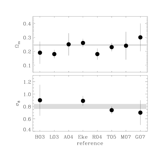
Figure 5: Recent estimates of $\Omega_{m}$ and $\sigma_{8}$ obtained via the Oort method or via the determination of $n(M,z)$ for optically-selected cluster samples. The shaded regions represent the WMAP 5-yrs allowed range for the same parameters [158]. References for the plotted points are: B03=[117], L03=[85], A04=[109], Eke=[128] (upper panel) or [159] (lower panel), R04=[124], T05=[147], M07=[90], G07=[48]. 1-$\sigma$ error bars (as given by the authors) are displayed. Note that, when needed, $\Omega_{m}$ has been estimated given $\sigma_{8}$ from [158] as a prior, and vice versa.

The first application of Oort’s technique probably dates back to 1965 when Abell [148] was able to constrain $\Omega_{m}$ in the interval $0.1-1.0$ (using number- rather than luminosity-density). The constraints based on this technique tightened significantly in the 1990’s, yielding $\Omega_{m}\simeq 0.2\pm 0.1$ and therefore indicating a low-density universe with high statistical significance [149, 150, 151, 152].

Another way of constraining the cosmological parameters is by estimating the number density of galaxy clusters (and superclusters), as a function of their mass, $n(M)$. Constraints on the combination of the $\Omega_{m}$ and $\sigma_{8}$ parameters can be obtained by comparing the observed $n(M)$ with theoretical predictions (e.g. [153, 154, 155]). The study of the evolution of $n(M)$ with $z$, $n(M,z)$, can provide even stronger constraints on cosmological models, allowing to break the $\Omega_{m}$–$\sigma_{8}$ degeneracy [156, 157].

Recent analyses of optically-selected cluster samples, some based on the Oort technique, some based on $n(M,z)$, provide estimates for $\Omega_{m}$ and $\sigma_{8}$ in agreement with the values obtained by WMAP 5-yrs [158] (see Fig. 5; [117, 85, 128, 124, 109, 147, 159, 90, 48]).

Superclusters can be used to constrain the evolution of cosmic structure in a more linear regime than applicable to galaxy clusters. It has been found that the Millennium simulation lacks very rich superclusters compared to the real universe [78]. Similarly, the existence of a very massive and compact supercluster recently detected at $z\simeq 0.9$ [134] is a rather unlikely event to be expected a priori in the currently favored cosmology.

While these results are encouraging, they are not yet competitive with those obtained with X-ray cluster surveys (see, e.g., [160]). However, X-ray cluster selection, as well as X-ray cluster mass estimates may suffer from their own systematics (see, e.g., [161, 162]). Moreover, at $z>1$ X-ray selection of clusters does not seem to be as efficient as IR selection [59, 50], and large samples of optical/IR-selected clusters are expected to come from ongoing and future very large ($\sim$ thousands of square-degrees) optical/IR surveys. Among these, the currently ongoing Red Sequence Cluster Survey 2, RCS-2 is the largest systematic search for galaxy clusters ever undertaken. It is based on the deg² MegaCam imager on the CFHT, it will image $\sim 1000$ deg² down to $g^{\prime}=25.3,r^{\prime}=24.8,z^{\prime}=22.5$, and will detect clusters of galaxies up to $z\sim 1$ using the CRS technique. It is estimated that upon completion, the survey will provide a sample of several thousand clusters. With such a sample it should be possible to constrain $\Omega_{m}$ to an accuracy of $\pm 0.02$ and $\sigma_{8}$ to an accuracy of $\pm 0.05$, and to estimate the equation of state of dark energy, $w$, to within 10% [163].

Other very ambitious surveys, most of them aimed at the characterization of the equation of state of dark energy and its evolution, are currently planned. They will prove very useful for distant cluster searches. A four-band survey is planned at the Panoramic Survey Telescope And Rapid Response System, Pan-STARSS, being developed at the University of Hawaii’s Institute of Astronomy. It will cover 1200 deg² down to $g=27$ in four bands. The Kilo-Degree Survey, KiDS, is a 1500 deg² public imaging survey in the five SDSS bands that will use the OmegaCAM instrument at the VLT Survey Telescope to go 2 magnitudes deeper than SDSS. It will be complemented by a near-IR survey, the VISTA Kilo-degree INfrared Galaxy survey, VIKING. The Dark Energy Survey, DES will cover 5000 deg² in 5 bands ($g,r,i,z,Y$) with a wide-field camera to be installed at the Blanco 4 m telescope at CTIO [164].

Not only imaging, also spectroscopic surveys are planned, from which catalogs of clusters of galaxies will probably be extracted. The Baryon Oscillation Spectroscopic Survey, BOSS, will observe 10,000 deg² and obtain redshifts for 1,5 million red luminous galaxies to $z=0.7$, using the SDSS 2.5m telescope and spectrographs. BOSS is part of the SDSS-III and should provide the first data-release in July 2011. Another planned spectroscopic survey (1 million galaxies in 100 nights) is the Hobby-Eberly Telescope Dark Energy Experiment, HETDEX.

From space, a significant increase in the number of $z>1$ clusters can come from a mid-IR survey to be conducted with the Spitzer Space Telescope during its warm mission , expected to last for about 2 years (see, e.g., [52]). In the longer term, an unprecedented amount of data may be provided by two proposed space-based missions, ESA’s Euclid, the merging of two proposed missions, DUNE and SPACE (see, e.g., [165]), and JDEM the Joint Dark Energy Mission of NASA and the U.S. Department of Energy. Euclid could provide $\approx 1.5\times 10^{8}$ galaxy redshifts down to $H_{AB}=22$, and a high-resolution, 3-filters, 20,000 deg² photometric survey of $\geq 2\times 10^{9}$ galaxies out to $z\sim 2$.

2 Structure and dynamics

Early determinations of cluster masses (e.g. [91, 92, 93]) from application of the virial theorem to cluster galaxy distributions, implicitly assumed that galaxies are fair tracers of the cluster gravitational potential, the so-called light traces mass hypothesis. However, the result of these analyses did not provide support for this assumption, since the derived masses were orders of magnitude larger than the sum of the masses of the visible galaxies. What if galaxies were not distributed like the total mass? Virial mass estimates could be biased high or low [95, 98]. Comparison with other cluster mass estimates [96, 104], and analyses of simulated clusters extracted from cosmological simulations [97] have since proven that the virial mass estimates are more or less correct. This then suggests that the projected spatial and velocity distribution of cluster galaxies is not very different from that of the total mass. However, proving this is not so simple, one must compare the distribution of the tracer population to the distribution of the total mass (see Sect. 2.3).

Knowing the mass distribution within clusters (also in relation to the distribution of the different cluster components) not only is important for a correct estimate of cluster masses, but also because it provides important clues on the formation and evolution of galaxy clusters and their components (e.g. [166, 167, 168]), and on the nature of DM (e.g. [169, 170, 171]). E.g. warm DM is expected to produce lower density halo cores than cold DM (CDM). If DM is cold, halos should be characterized by density profiles with a central cusp, such as the NFW profile [172],

$$\rho_{NFW}=\frac{\rho_{0}}{(cr/r_{200})(1+cr/r_{200})^{2}},$$ (6)

where $c$ is the concentration parameter. Modifications of the NFW profile have been suggested, all characterized by the central cusp [173, 174, 175]. Another widely used cuspy density profile is the Hernquist model [176],

$$\rho_{Hernquist}=\frac{\rho_{0}}{r\,(r+r_{H})^{3}}.$$ (7)

On the other hand, observations of galaxy rotation curves have revealed the presence of a central core (e.g. [177, 178, 179, 180, 181]). Cores could be created in the mass distribution if the DM particles are self-interacting [169], or if galaxies are able to pump energy into the DM component via dynamical friction [146, 182]. Cored mass density models have been suggested [183, 184], such as the Burkert profile,

$$\rho_{Burkert}=\frac{\rho_{0}}{(1+r/r_{c})[1+(r/r_{c})^{2}]},$$ (8)

characterized by the core radius $r_{c}$. Another widely used mass profile is the softened isothermal sphere,

$$\rho_{SIS}=\frac{\rho_{0}}{1+(r/r_{c})^{2}}.$$ (9)

Note that at large radii $\rho_{Burkert}\propto r^{-3}$ like the NFW profile, while $\rho_{SIS}\propto r^{-2}$.

Given the problems that the NFW model has at small scales, it is important to test its validity on larger scales, i.e. on cluster- and group-sized halos. Hence determination of the cluster mass profile, $M(r)$, becomes a crucial test for the CDM cosmological model (see Sect. 2.2).

2.1 Dynamical analysis: methods

The most commonly used method to determine the mass profile $M(r)$ of galaxy clusters is the Jeans method (see [86]) hereafter described.

Assuming spherical symmetry, the projected number density profile $N(R)$ of a tracer can be uniquely deprojected via the Abel inversion equation [86],

$$\nu(r)=-\frac{1}{\pi}\int_{r}^{\infty}\frac{dN}{dR}\frac{dR}{\sqrt{R^{2}-r^{2}}},$$ (10)

where $\nu(r)$ is the 3-d number density profile, $R$ and $r$ are the projected and, respectively, the 3-d radius (i.e. the distance from the cluster center). While this deprojection is straightforward, deprojecting the line-of-sight velocity dispersion profile, $\sigma_{v}(R)$, requires knowledge of the velocity anisotropy profile,

$$\beta(r)\equiv 1-\frac{\rm{<}v_{t}^{2}\rm{>}(r)}{\rm{<}v_{r}^{2}\rm{>}(r)},$$ (11)

where $\rm{<}v_{r}^{2}\rm{>}(r)$, $\rm{<}v_{t}^{2}\rm{>}(r)$ are the mean squared radial and tangential velocity components, which we can write as $\sigma_{r}^{2}(r)$ and $\sigma_{t}^{2}(r)$ respectively, in the absence of bulk motions and net rotation. In the simplest case of the isotropic velocity distribution, $\beta(r)\equiv 0$, the $\sigma_{v}$ deprojection reads

$$\sigma_{r}^{2}(r)=-\frac{1}{\pi\nu(r)}\int_{r}^{\infty}\frac{d[N\,\sigma_{v}^{2}]}{dR}\frac{dR}{\sqrt{R^{2}-r^{2}}}.$$ (12)

Through a more complicated set of equations it is possible to deproject $\sigma_{v}$ in the case of generic $\beta$ [185].

Given $\sigma_{r}(r)$ and $\beta(r)$ it is possible to determine the mass profile, $M(r)$, through the Jeans equation for a collisionless system of particles (e.g. galaxies),

$$M(r)=-\frac{r\sigma_{r}^{2}}{G}\left(\frac{d\ln\nu}{d\ln r}+\frac{d\ln\sigma_{r}^{2}}{d\ln r}+2\beta\right).$$ (13)

Similarly, given $M(r)$ and $\beta(r)$ it is possible to determine the observed, projected phase-space distribution of the tracers via

$$\nu(r)\,\sigma_{r}^{2}(r)=G\int_{r}^{\infty}\frac{\nu M}{\xi^{2}}\,\exp\left[2\int_{r}^{\xi}\frac{\beta dx}{x}\right]d\xi,$$ (14)

and

$$N(R)\sigma_{v}^{2}(R)=2\int_{R}^{\infty}\left(1-\beta\frac{R^{2}}{r^{2}}\right)\frac{\nu\,\sigma_{r}^{2}\,r\,dr}{\sqrt{r^{2}-R^{2}}}.$$ (15)

From the eqs. above it is clear that the same observed number density and velocity dispersion profiles $N(R)$ and $\sigma_{v}(R)$ can be obtained by a different combination of the mass and anisotropy profiles $M(r)$ and $\beta(r)$, and vice versa. Symmetrically, given the observables $N(R)$ and $\sigma_{v}(R)$ it is possible to obtain $M(r)$ only if $\beta(r)$ is known and $\beta(r)$ only if $M(r)$ is known [185, 186, 187, 188]. This is the so-called “mass–anisotropy” degeneracy.

In order to break this degeneracy, one must constrain $\beta(r)$ independently from $M(r)$. A possibility is to build distribution function models (see, e.g., [189]) and use them to compute the probability that a particle observed at a given projected radius $R$ have a line-of-sight velocity $v$ in a given interval $dv$. These probabilities are then used in a maximum likelihood analysis to determine the model that best represents the observed projected phase-space distribution of galaxies. The best-fit model can also be chosen by comparing the line-of-sight velocity distribution predicted by the model with the observed histogram of velocities of cluster galaxies. The comparison in this case can be done by considering moments of the velocity distribution higher than the second (e.g. [98, 189, 190, 191]). Robust estimates of these moments are obtained by the use of Gauss-Hermite polynomials.

Another way to break the mass–anisotropy degeneracy is to consider several independent tracers of the gravitational potential, then apply the Jeans procedure independently for each of the tracers. Subject to the constraint that different tracers should provide identical $M(r)$ solutions, it is possible to reduce the range of acceptable $[M(r),\beta(r)]$ (see, e.g., [192]).

The Jeans procedure outlined above also assumes that the system is in dynamical equilibrium. However, since clusters grow by accretion of field galaxies (e.g. [193, 100]) they are not steady-state systems. One should then include the time derivative term in the Jeans equation (eq. 4-29c in [86]). Fortunately, the rate of mass accretion onto low-$z$ clusters is small, $\simeq 8$% of the total mass in a dynamical time ($\sim 1/10$ the Hubble time) [194], although it increases with redshift [195]. Since the accretion process is not smooth, some clusters, even at low-$z$, may be observed during an intense accretion phase. These clusters are nevertheless easy to spot, since most of the accreted mass is in the form of groups [196] which can be identified as substructures in the projected phase-space distribution of cluster galaxies (see Sect. 2.5). More problematic is the case of galaxy groups [197] and of high-$z$ galaxy clusters, since several of these systems are likely to be detected when they are still in their collapse phase and far from dynamical equilibrium.

Other usual assumptions of the Jeans analysis are sphericity and the absence of net rotation. Deviation from spherical symmetry has been shown not to be a major problem for individual clusters [189, 198] and there is little if any evidence for net rotation in galaxy clusters [199].

The Jeans equation applies to a collisionless system of particles. Galaxies do behave as quasi-collisionless particles when they move at high speed, which is the case in galaxy clusters. High-speed galaxy encounters produce little tidal damage and do not lead to mergers [200], and only the most massive galaxies have their motions slowed down by dynamical friction [201]. As the mass of the host system of galaxies decreases, dissipative processes become more important. Groups in particular, are very favorable sites for galaxy mergers [139] so the collisionless Jeans equation may not be applicable for these systems [202].

Interlopers are another serious problem when one is trying to determine a cluster mass profile. Interlopers are foreground/background galaxies that happen to lie in the same projected phase-space region occupied by cluster galaxies. Several methods exist to get rid of them. Tests on cluster-scale halos extracted from cosmological simulations have shown these methods to perform relatively well (see in particular [97, 203, 204]). There are however interlopers that are impossible to distinguish from real cluster galaxies; in order to deal with these interlopers a statistical approach is generally adopted (e.g. [203]). In the statistical approach the projected phase-space distribution of galaxies observed in the cluster region is assumed to be contaminated by a certain fraction of interlopers with a well known spatial and velocity distribution (inferred from the analysis of simulated halos). Alternatively, one can use galaxy internal properties, such as, e.g., colors, spectral types, and morphologies, to improve the separation between cluster and field galaxies.

In order to determine a reliable cluster mass from the projected phase-space distribution, $\geq 60$ galaxies are needed [97], but about an order of magnitude more are required for the determination of a cluster mass profile (see, e.g., [205]). Spectroscopic samples of several hundred member galaxies per cluster are still rare, hence it is common practice to build a ’composite’ cluster by stacking together the data of several clusters (see, e.g., [151, 189, 206, 207, 208]). The projected phase-space distributions of different clusters can be put together by scaling galaxy radii and velocities with virial quantities ($r_{200},v_{200}$). This procedure is supported by the results of cosmological numerical simulations, that suggest that halos at the cluster mass scale are a quasi-homologous family of objects, their mass profiles changing only slightly with the halo mass [172, 209].

By stacking clusters together it is possible to deal with samples of a few thousand cluster galaxies. These samples are obtained from cluster-dedicated spectroscopic surveys, such as ENACS [4, 5] and the CNOC [210, 211], and also from field spectroscopic surveys wherein clusters have been identified, such as the 2dFGRS [212, 213] and the SDSS (see e.g. [56, 214]). The most recent cluster-dedicated spectroscopic surveys are the Las Campanas/Anglo Australian Telescope Rich Cluster Survey (LARCS [215]), the Cluster and Infall Region Nearby Survey (CAIRNS [216]), the WIde Field Nearby Galaxy-clusters Survey (WINGS [217]), and the EDisCS [71].

In recent years, another technique, usually referred to as the Caustic method ([218, 219]) has been developed. In this method, a cluster $M(r)$ is obtained from the amplitude of the caustics delineated by the projected phase-space distribution of galaxies in the cluster region. This amplitude is related to the gravitational potential through a function ${\cal F}$ of the projected radius, $R$, of the gravitational potential, and of $\beta(r)$ (see eqs. 9 and 10 in [219]). Also this method suffers from the mass–anisotropy degeneracy, but only in the central cluster regions, since numerical simulations indicate ${\cal F}\approx\rm{const}$ at large radii, $R>r_{200}$ (see Fig. 2 in [219]). Hence the Caustic mass estimate is relatively robust at large radii, exactly where the Jeans estimate may be more affected by problems of interlopers and deviations from dynamical equilibrium. On the other hand, the Jeans method is more robust at small radii, where imperfect knowledge of ${\cal F}$ increases the systematic uncertainty in the Caustic mass estimate.

The Caustic and Jeans methods have been shown to produce consistent cluster mass profiles [206, 216]. Through analyses based on samples of cluster-sized halos extracted from cosmological numerical simulations, both methods have been shown to be reliable [219, 198, 205]. There are only a few direct comparisons of mass profiles determined from the distribution of cluster galaxies with those determined using the X-ray-emitting intra-cluster gas or via gravitational lensing. In general, lensing mass profiles are in agreement with those determined via the Caustic [220] and Jeans [221] methods. On the other hand, the agreement is less good between X-ray determined mass profiles and those determined from the distribution of cluster galaxies [220, 222].

2.2 Mass profiles

Application of the Caustic technique to the CAIRNS sample [223, 224, 225, 216, 124] has shown that the cluster mass density profile $\rho(r)$ resembles the NFW model, except at large radii, $r>2\,r_{200}$, where its slope seems to be somewhat steeper (between $-3$ and $-4$). SIS models are rejected. The best-fit values of the NFW concentration parameter range between 5 and 17. Very similar results have recently been obtained by application of the same Caustic technique to a new sample of 72 X-ray selected clusters extracted from the SDSS (the CIRS sample [214]).

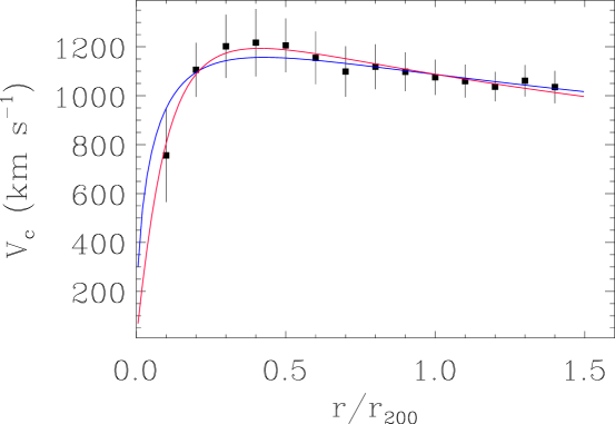
Figure 6: The DM circular velocity profile ($V_{c}=\sqrt{GM/r}$) of the stacked cluster from the ENACS data-set [227] (points with 1-$\sigma$ random $+$ systematic error bars). The best-fitting NFW and Burkert models are indicated with a blue and red line, respectively.

A combination of the Jeans and Caustic analysis was used to determine the mass profile of a composite cluster extracted from the 2dFGRS [206]. By stacking together 43 nearby clusters, a total sample of 1345 cluster galaxies was obtained. Late-type galaxies (LTGs in the following) were excluded from the sample, and isotropy was assumed for the Jeans analysis. The resulting $M(r)$ was found to be well described by a $c\simeq 6$ NFW profile over the radial range 0–2 $r_{200}$. If a cored profile is fitted to $M(r)$, the core radius is constrained to be small, $<0.1\,r_{200},$ i.e. not much larger than the size of the BCG which generally sits at the cluster center.

A composite of 1129 ETGs was constructed from 59 clusters from the ENACS sample [207]. By comparing the velocity distribution of cluster ETGs with distribution function models, stringent constraints on $\beta$ were obtained. The ETGs were shown to move on nearly isotropic orbits, hence $\beta\equiv 0$ was adopted in the Jeans analysis. It was found that $\rho\propto r^{-2.4\pm 0.4}$ at $r=r_{200}$, fully consistent with the NFW asymptotic slope. Two models were shown to provide an adequate fit to the data, a NFW profile with $c=4\pm 2$, and a Burkert profile with a rather small core radius ($\leq 0.1\,r_{200}$). The $M(r)$ solution obtained by using ETGs as isotropic tracers was later confirmed by using another tracer of the gravitational potential, i.e. cluster Sa–Sb galaxies [226].

The mass distributions of a few individual nearby clusters (including Coma) have also been determined [190, 205, 204]. In order to break the mass-anisotropy degeneracy not only the projected velocity dispersion profile but also the velocity kurtosis profile were derived and modeled. All cluster mass profiles turned out to be well described by an isotropic NFW model, with a median$(c)=7$.

The ENACS data-set was re-analyzed to determine the relative contributions of baryons and DM to the total mass profile [227]. Since the DM contribution is dominant, the resulting DM $M(r)$ does not differ significantly from the total mass $M(r)$, it is only slightly more concentrated (NFW $c=5\pm 1$, Burkert $r_{c}=0.12\pm 0.02$; see Fig. 6). If the subhalos DM contribution is subtracted from the whole DM component, what is left is the diffuse DM associated with the main halo (cluster), which appears to be even more concentrated (NFW $c=7\pm 1$, Burkert $r_{c}=0.09\pm 0.02$). Note however that splitting the DM $M(r)$ into its halo and subhalo components is very model-dependent.

Figure 7: The velocity anisotropy $\sigma_{r}/\sigma_{t}$ vs. the NFW concentration $c\equiv r_{200}/r_{s}$ parameter as determined for a stacked sample of 26 X-ray-emitting small groups, mostly from the GEMS sample [139]. 1-$\sigma$ contours are shown [234].

These results show that central cuspy models such as NFW and Hernquist provide an adequate fit to the mass profile of nearby galaxy clusters. The Burkert profile is also acceptable, as far as the core radius is small, of order the size of the BCG or smaller. Since galaxies are treated as point-like tracers of the potential in the Jeans analysis, the size of the core radius is close to the resolution size of the analysis. The upper limit on the size of the core radius can be used to constrain the DM scattering cross section by comparison with simulations [170]. The resulting upper limit, $<2$ cm² g^-1, effectively rules out Self-interacting DM as a possible way to explain the cored mass density profile of dwarf galaxies [169, 228]. The absence of a significant core in the cluster mass distribution also implies that dynamical friction is not very effective in transferring cluster galaxy kinetic energy to DM particles [182]. This is consistent with observational estimates of galaxy luminosity segregation in clusters (see, e.g., [99]).

While the inner slope of the density profile is essentially unconstrained, at large radii the asymptotic slope of the density profile is constrained to lie between $-3$ and $-4$, consistent with the NFW, Hernquist, and Burkert models, but not with the SIS model.

At higher redshifts the constraints are less strong. Results based on the analysis of 16 stacked CNOC clusters confirm that NFW is an acceptable mass profile model on cluster scales also at $0.17\leq z\leq 0.55$ [151, 229, 189].

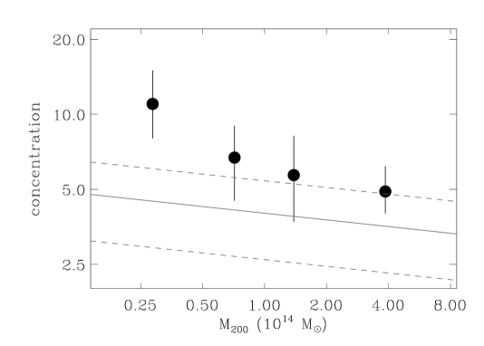
Figure 8: The NFW concentration $c\equiv r_{200}/r_{s}$ parameter vs. the virial mass $M(r_{200})$ as determined on four samples of groups and clusters [234, 230, 206, 227] characterized by different average masses (points with 1-$\sigma$ error bars). The solid and dashed lines indicate the median and $\pm 1$-$\sigma$ predictions for a $\Lambda$CDM cosmology with WMAP5 cosmological parameters [235].

The CDM-motivated NFW model fits well the mass profiles of cluster-sized halos, and does not fit the mass profiles of galaxy-sized halos. Hence it is important to test the model at intermediate scales (groups of galaxies). Unfortunately, the results for the group $M(r)$ are still controversial so far. From the analysis of 588 galaxies in 20 stacked groups the group density profile was found to be consistent with the Hernquist model [230], but using a sample twice as large the same authors concluded that a single power-law model is a better representation of the data [231]. Both results are inconsistent with those obtained for a higher redshift group sample ($0.1\leq z\leq 0.55$) whose average mass density profile is characterized by a very shallow-slope and a central core [42].

Discrepant results probably arise as a consequence of different selections of the group samples, since not all groups are dynamically virialized systems [197, 232, 200, 230]. A proper characterization of the group mass profile awaits a careful definition of the group sample, based on the group characteristics. Such a sample may be provided by the groups of the Group Evolution Multiwavelength Study (GEMS [139]) for which both X-ray and optical data are available. Comparing optical and X-ray group properties helps constraining the group dynamical status [129]. A preliminary analysis of this sample suggests consistency of the average group mass profile with the NFW model, with a higher concentration parameter than for clusters, in line with predictions from $\Lambda$CDM (see Fig. 7; [233, 234]).

In Fig. 8 results for the best-fit NFW concentration parameter are collected from the literature. The $c=c(M)$ trend is somewhat above recent predictions from $\Lambda$CDM cosmological numerical simulations [235].

2.3 The relative distribution of dark and baryonic matter

In order to answer the question raised in Sect. 2, i.e. are galaxies distributed like the DM, the mass density profiles of galaxy systems must be compared with their galaxy number- or luminosity-density profiles. These can be evaluated by counting galaxies or, respectively, summing galaxy luminosities, in concentric annuli around the cluster center, taking into account the completeness correction, if needed. The mass-density to luminosity- (or number-) density profiles ratio is called the mass-to-light ($M/L$) profile.

Since different cluster galaxy populations have different distributions (see Sect. 3.1) there is not a unique $M/L$ profile. Depending on the photometric band used to select the cluster galaxies, the relative fraction of red and blue, quiescent and star-forming, early- and late-type galaxies in the resulting sample may vary. Modulo the selection in type or color, the $M/L$ profiles found by different authors are generally in agreement [206, 207, 124, 227]. The cluster $M/L$ profile increases from the center to $0.2\,r_{200}$, flattens out to $r_{200}$, and then decreases, by a factor $\times 2$ out to the turnaround radius. The trend near the center is caused by the presence of the BCG which sits at the bottom of the cluster potential well. The external, decreasing trend is instead caused by the increasing fraction of late-type, blue galaxies with radius. Selecting only the red, early-type, quiescent cluster galaxies (or selecting galaxies in the $K$ band) flattens the $M/L$ profile in the outer parts. Removing the BCG flattens the $M/L$ profile near the center. Hence, the light of red cluster galaxies (except the brightest one) does indeed trace the mass, but the light of blue cluster galaxies does not. Applying the virial theorem to the distribution of red cluster galaxies (BCG excluded) should then provide unbiased mass estimates for dynamically relaxed clusters [97].

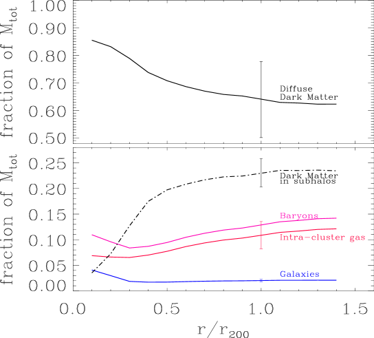
Figure 9: The fractional mass distributions of the different components of galaxy clusters, i.e. diffuse DM, DM associated with subhaloes, and baryons (intra-cluster gas plus galaxies) [227]. Representative 1-$\sigma$ (random $+$ systematic) error bars are indicated.

While galaxies are useful tracers of the cluster potential, they are by far a negligible component not only of the cluster mass, but also of the baryonic mass. Most of the baryonic mass is in the intra-cluster, X-ray emitting gas. The intra-cluster gas-to-total mass fraction increases with radius as $r^{0.4}$ [227]. Hence, the baryonic mass is less concentrated than the total mass at all radii, except near the very center, where the baryons of the BCG dominate the mass budget (see Fig. 9).

Exploring the evolution of the $M/L$ profile with redshift can provide useful information on when and how the different galaxy populations settle in galaxy clusters. The poor constraints existing so far for clusters at $z\approx 0.3$ seem to confirm that $M/L\approx$ constant out to the virial radius, when only red galaxies are selected [189].

Since the average mass profile of low-mass galaxy systems (groups) is not yet well constrained, results on their $M/L$ profile are controversial [230, 42]. Cosmological numerical simulations indicate that groups have more concentrated mass profiles than clusters (see e.g. [172, 209]), while observations indicate that groups have less concentrated galaxy number density profiles than clusters [126], hence groups might be characterized by steeper $M/L$ profiles than clusters.

2.4 The orbits of galaxies and mass accretion

According to the hierarchical model for the formation and evolution of cosmic structures, clusters grow from accretion of galaxies and galaxy groups from the field. CDM cosmological numerical simulations have shown that DM particles accrete onto clusters on moderately radially elongated orbits, i.e. with a radial velocity anisotropy that increases moving out to the virial radius (e.g. [236, 237, 219, 238]). Observational evidence supporting the hierarchical build-up of galaxy clusters has been provided by the discovery that cluster ETGs and LTGs have different kinematics [193, 239, 201, 151, 100]. LTGs are characterized by a larger $\sigma_{v}$ than ETGs, and this has been interpreted as evidence that LTGs are an infalling, unvirialized population. However, kinematical evidence alone cannot prove the LTGs are indeed an infalling population, full dynamical modeling is required (see Sect. 2.1).

One of the first full dynamical modeling of a cluster was made in the early 80s for the Coma cluster [240]. It was concluded that the galaxy orbits are not primarily radial. Consistently, many recent dynamical modeling of low-$z$ galaxy clusters, mostly based on stacked cluster samples from the ENACS, CNOC, and SDSS data-sets, have concluded for quasi-isotropic orbits of ETGs [229, 230, 241, 190, 207]. Since ETGs are the dominant cluster galaxy population, also the mean velocity anisotropy (see eq. 11) of cluster galaxies altogether is found to be $\beta\approx 0$ [189, 216, 205]. Interestingly, full dynamical analysis does not support the interpretation of LTGs as an unvirialized infalling population. Probably the details of the results depend on how accurately are interlopers rejected from the sample of cluster members. Anyway, both for nearby and medium-$z$ clusters LTGs are found to be in dynamical equilibrium within the cluster potential. At variance with ETGs, however, LTGs have moderately radially anisotropic orbits [229, 230, 241, 226, 242], with an anisotropy that increases with radius [226, 233, 243] (see Fig. 10). A finer distinction of the LTG population into two classes, Sa–Sb on one side and Sbc–Irr on the other, has shown that the radial anisotropy is characteristic of the latter class only, while the orbits of Sa–Sb are isotropic within observational uncertainties [226].

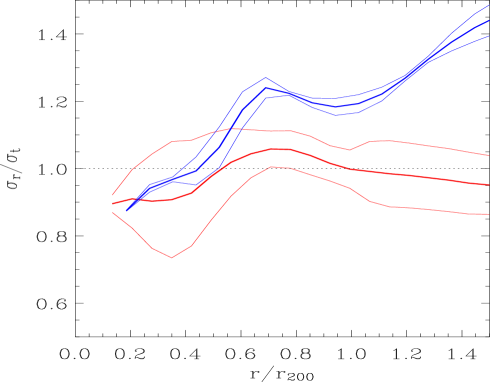
Figure 10: A preliminary determination of the velocity anisotropy profiles of the red and blue galaxies in the CIRS clusters and their $\pm 1$-$\sigma$ confidence levels [243].

The velocity anisotropy profile of LTGs is remarkably similar to that of DM particles in clusters extracted from cosmological numerical simulations (see, e.g., [237, 219, 238]). The orbital characteristics of DM particles are reminiscent of their almost radial accretion onto clusters along the surrounding filaments. By analogy, also the predominantly radial orbits of LTGs can be taken as an indication that these galaxies retain the dynamical memory of their infalling motions into the clusters. They are probably newcomers of the cluster environment, where they have spent too little time for the dynamical memory of their initial infall to be totally erased. ETGs, on the other hand, have had time to undergo sufficient energy and angular momentum mixing, capable of isotropizing their orbits (see, e.g., [244] and references therein). Such energy and angular momentum mixing occurs in galaxy systems mostly via phase- and chaotic-mixing or violent relaxation [245, 246, 247, 248, 249], which occur when the system gravitational potential changes rapidly, i.e. at the time of the system assembly or on the occurrence of major mergers [250, 251, 252]. Another process capable of isotropizing galaxy orbits is the secular growth of cluster mass [101].

LTGs have probably entered the cluster environment after the last major merger. Consistent with this hypothesis is the fact that they still retain most of their gas content, which cluster-related environmental processes will eventually strip given sufficient time (see Sect. 3.6). Numerical simulations confirm that recently accreted satellites in a host halo have more radially extended and less bound orbits [253, 254].

Independent, direct evidence for the accretion of field spirals (S) onto clusters has been obtained from the analyses of the distance–velocity diagram around the Virgo clusters and other nearby galaxy systems [255, 256, 257]. Unfortunately, distance measurements are affected by large uncertainties and cannot yet be used to assess the infall process in a statistically significant sample of massive clusters.

There is no direct estimate of the evolution with $z$ of the ETG and, separately, the LTG $\beta(r)$. However, an indirect argument can be used to rule out significant evolution at least up to $z\simeq 0.3$. The projected phase-space distributions of ETGs and, separately, LTGs in the $z\simeq 0.1$ ENACS clusters and in the $z\simeq 0.3$ CNOC clusters are remarkably similar [233], except for the normalization (the fraction of blue galaxies is higher in more distant clusters, the so-called Butcher-Oemler effect – see Sect. 3.2). Also the average $M(r)$ of ENACS and CNOC clusters are very similar [207, 189]. Similarity of the observed projected phase-space distributions and of the mass profiles then imply, from the Jeans analysis (see Sect. 2.1), similarity of the velocity anisotropy profiles. This implies, in particular, that, just like their low-$z$ counterparts, also the CNOC LTGs are newcomers of the cluster environment. Given that their fraction decreases with time, cluster LTGs must either transform in ETGs or dim with time (or both). If they do undergo color and morphological transformation, they need at the same time undergo orbital isotropization since ETG orbits are isotropic and LTG orbits are moderately radial. This observation could prove useful in constraining the mechanisms that drive galaxy evolution in clusters (see Sect. 3.6).

The mass accretion rate can be estimated by measuring the mass outside the virial cluster region which is bound to infall into the cluster in the future. Using the Caustic method it has been estimated that $M(r<r_{200})\approx M(r_{200}<r<r_{t})$, where $r_{t}\approx 5\,r_{200}$ is the turnaround radius, i.e. the characteristic radius that separates accretion from outflow regions [214]. According to $\Lambda$CDM cosmological N-body simulations, clusters will reach their final $M_{200}$ mass when they are 32 Gyr old [258]. The Caustic estimate then implies a future average accretion rate of $\dot{M}\approx 0.06\,M_{200}/\mbox{Gyr}$. This estimate is in excellent agreement with an independent estimate obtained by summing up the mass of recently accreted groups in the Coma cluster [194], $\dot{M}\simeq 0.02-0.11\,M_{200}/\mbox{Gyr}$. The analysis of the density profiles of cluster galaxies in different redshift bins has allowed estimates of the stellar mass accretion rates [195] , $\dot{M_{\star}}\sim 0.06\,M_{\star}/\mbox{Gyr}$ at $z=0.45$ and $\dot{M_{\star}}\sim 0.02\,M_{\star}/\mbox{Gyr}$ at $z=0.20$, implying a significant $z$-evolution of the mass accretion rate. These estimates depend on the timescale for halting star formation (SF in the following) in the accreting blue galaxies, assumed here to be $\sim 1$ Gyr. A timescale of $\sim 0.5$ Gyr would double these estimates, and make them more similar to those obtained by the other techniques mentioned above.

2.5 Subclusters

In Sect. 2.4 evidence has been provided that clusters evolve by accreting galaxies from the surrounding field. A large fraction of field galaxies occur in groups, hence in fact clusters not only accrete isolated galaxies but also groups of galaxies. When groups of galaxies enter the cluster environment they are subject to tidal forces that tend to disrupt them (see, e.g., [259, 260, 261]). The time of disruption is longer for less massive groups [260, 261], that can resist for several Gyr [260, 262]. Observationally, groups accreted by clusters and not yet totally disrupted will appear as secondary, statistically significant overdensities in the distribution of cluster galaxies. They are usually called “subclusters” or cluster “substructures” (see [263] for a review).

In reality, not all observationally-identified subclusters are the surviving remnants of galaxy systems which have been accreted into a cluster gravitational potentials. Groups that are in the cluster foreground or background can also be identified as local galaxy overdensities, and hence confused with real subclusters. Among the foreground and background groups, those that are dynamically bound to the cluster will eventually be accreted and become real subclusters in the future [264].

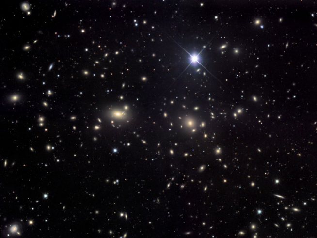
Figure 11: The central region of the Coma cluster ($1.13\times 0.65$ Mpc² at the cluster redshift, $z=0.0233$) displaying a clear bimodal distribution of galaxies concentrated around the two BCGs (from http//www.mistisoftware.com/astronomy/Galaxies_ComaCluster.htm).

It is important to identify and study subclusters. They provide information on the accretion process itself and ultimately serve as constraints to cosmological models (see, e.g., [265, 266]). For instance, the total mass of subclusters in the Coma cluster region (see Fig. 11) has been used to provide an estimate of the Coma cluster accretion rate (see Sect. 2.4). The distribution of subcluster luminosities has been compared to the distribution of subhalo masses thereby providing a test for theories of structure formation [267]. In the so-called ’bullet’ cluster the distributions of the total and baryonic masses are displaced as the result of a very energetic collision of the cluster with an infalling group [268]. A measure of this displacement has been used to set an upper limit to the cross-section of DM particles [269, 270].

Another aspect of the importance of subcluster studies is that internal cluster dynamics can be affected by the very energetic ($\sim 10^{55}$ J) cluster–subcluster collisions. Part of the energy and of the angular momentum of the collision is transferred to the cluster and subcluster galaxies. As a consequence, the collision affects the velocity distribution of cluster members, typically broadening, skewing, and/or flattening an initially Gaussian distribution [271, 272], but also generating mean velocity gradients along the collision axis [273, 274]. Also the spatial distribution of galaxies is affected, and becomes less centrally concentrated [272, 99]. As a consequence, cluster masses and velocity dispersions are generally overestimated during and some time after the collision (see, e.g., [275, 272, 97]). Typically, masses are overestimated by $\sim 30$%, but depending on many parameters (e.g. the relative angle of the collision and line-of-sight axes, the mass ratio of the subcluster and main cluster, the time after the collision, the observational sampling, etc.) the mass can be overestimated by up to a factor $\sim 5$ or even underestimated by a factor $\sim 3$ in extreme cases [272, 97].

Cluster–subcluster collisions can also have important effects on galaxy properties. They produce rapid variations in the cluster gravitational field that can stimulate non-axisymmetric perturbations in the galaxies involved in the collisions, and increase the rate of galaxy–galaxy interactions, leading to bursts of SF [276, 277, 278, 279]. Moreover, collisions are likely to displace the central BCG from the bottom of the cluster potential well, thus effectively halting the accretion process of satellite galaxies onto the BCG (see, e.g., [280, 281, 267]).

Several methods have been developed to identify subclusters in the optical (see, e.g., [272] and [263]). Depending on the data-set, the different methods are more or less effective. Generally speaking, all these methods look for deviations from symmetry in the spatial and/or velocity distribution of cluster galaxies, or for significant secondary peaks in the surface density or projected phase-space distributions.

The most widely used of these techniques has been developed in the late 80s [282]. In its original formulation, the method consists in considering all possible subgroups of 10 neighbors around each cluster galaxy. The mean velocities and velocity dispersions of all these subgroups are calculated, as well as their differences with respect to the corresponding global cluster quantities. The sum of the squares of these differences constitutes the $\Delta$ statistics,

$$\Delta=\sum_{i=1}^{N}(11/\sigma_{v}^{2})[(\overline{v}_{i}-\overline{v})^{2}+(\sigma_{i}-\sigma_{v})^{2}],$$ (16)

where $\sigma_{v}$ and $\overline{v}$ are the velocity dispersion and mean velocity of the whole cluster, $\sigma_{i}$ and $\overline{v}_{i}$ are the corresponding quantities for any group $i$ of 11 galaxies, and the sum is over all $N$ cluster galaxies. Montecarlo simulations are then run to establish the statistical significance of $\Delta$.

After its original formulation, this method has been modified and adapted by several authors [283, 284, 99]. This was done in particular for extending the scope of the method, initially meant to estimate the probability that a cluster contains subclusters, and later adapted to find which galaxies have the highest likelihoods of residing in subclusters.

Among clusters analyzed with the $\Delta$ technique, $\simeq 1/3$ show significant evidence for subclustering, both at low and medium-to-high redshifts (see, e.g., [100, 285]). A similar fraction has been found with other techniques (see, e.g., [286, 115]), but this fraction is likely to be a lower limit, since other, deeper analyses have discovered subclusters in clusters previously thought to contain none (see, e.g., [284, 267]). Presumably any cluster would show evidence for subclustering if examined in sufficient detail, because of the very nature of the process by which these objects form (hierarchical clustering). Today’s analyses are aimed at determining not the fraction of clusters with subclusters, but the mass distribution of subclusters [267] and its redshift evolution, and to compare it with the prediction of cosmological numerical simulations, in order to learn about the process of structure formation and evolution.

Other constraints can come from comparing the observed distribution of subclusters in clusters with that predicted by cosmological models. Observational estimates of the number density profile of subcluster galaxies agree with estimates from $\Lambda$CDM cosmological numerical simulations [226, 261]. Moreover, the subcluster orbits are found to be tangential [226], which is consistent with the idea that subclusters on radially elongated orbits are selectively destroyed by tidal effects [253, 287].

2.6 Summary and perspectives

The analyses of cluster dynamics based on galaxies as tracers of the gravitational potential have come to the following conclusions.

• $M(r)$ is consistent with the prediction of CDM cosmological numerical simulations.

• A cored $M(r)$ is not excluded, but the core, if exists, has to be small, of order the size of the central bright galaxy, essentially ruling out self-interacting DM as a way to explain galaxy rotation curves.

• At large clustercentric radii, $r\geq 2r_{200}$, the mass density profile slope is $\simeq-3.5\pm 0.5$, still consistent with NFW, but somewhat steeper.

• The red/early-type/passively-evolving cluster galaxies are characterized by nearly isotropic orbits, while the blue/late-type/star-forming cluster galaxies have increasingly radial anisotropy with increasing clustercentric radius.

There is a lot that remains to be done and that will be made possible by exploiting already existing and forthcoming databases, such as the Imacs Cluster Building Survey. The constraints that have been obtained so far can be put on a more solid statistical basis. E.g. it should be possible to rule out either the cuspy NFW or the cored Burkert with a $\sim 5$ times larger data-set than the ones used so far. The currently loose constraints on the relation between mass and concentration can be made tighter, in order to confirm or reject the apparent (albeit marginal) discrepancy with the theoretical predictions [288, 235]. While constraints on the shape of $c=c(M)$ relation can only come by sampling the group mass scales, constraints on the normalization can also come by sampling the cluster mass scales alone, where kinematical methods are more powerful (because the number of available galaxies per cluster is larger). On the other hand, constraining the group $M(r)$ is extremely important by itself, since group masses are intermediate between cluster masses, where cosmologically motivated $M(r)$ models appear to work, and galaxy masses, where they do not.

Individual cluster samples with $\geq 500$ galaxy velocities are currently rare. With future, larger samples it will become possible to constrain individual cluster concentrations and eventually compare the $c$-distribution of a complete cluster sample with theoretical predictions, which indicate a skewed distribution (e.g. [289]). Maybe it will even be possible to check whether it is indeed the concentration that changes from cluster to cluster, or whether it is the shape of the density profile [290, 291].

Models and simulations indicate that cluster mass profiles depend on their accretion history [292, 293, 294, 295, 296]. This could be tested by characterizing the mass profiles of galaxy clusters as a function of their degree of internal dynamical relaxation (or, inversely, of subclustering). Determining the detailed properties of subclusters in a complete cluster sample can provide another interesting test of cosmological models. Knowledge of the cluster and subcluster masses, and their relative velocities is required [297].

With a substantially larger data-base that the ones used so far, it will also be possible to determine orbital constraints for several classes of cluster galaxies, distinguished by color and internal structure. These are galaxy properties that are unlikely to evolve simultaneously (see Sect. 3.2) and orbital isotropization can be used as a clock for galaxy evolution in clusters. It is also important to determine the orbital characteristics of different cluster galaxy populations as a function of cluster mass and/or cluster structure, since orbital isotropization may occur at different epochs and proceed with different speeds depending on the global cluster properties. As a matter of fact, in some clusters ETGs and LTGs move with similar orbital anisotropies [242].

Numerical simulations and analytical models predict that the shapes of the mass-density and anisotropy profiles of cosmological halos are closely related [298, 299, 300]. With current data-sets it is not possible to independently constrain cluster mass- and anisotropy-profiles to the accuracy level required to test this predictions, but with future, larger data-sets, it will.

Investigating the redshift evolution of cluster mass- and anisotropy-profiles and of cluster mass accretion can provide interesting constraints on the hierarchical model of cluster formation and galaxy evolution in clusters. Cosmological numerical simulations predict two phases of CDM halo assembly. The initial gravitational collapse phase is responsible for establishing the central slope of the mass density profile, while the external slope is established by the later accretion phase [244, 249]. It should then be possible to test this evolutionary scenario by determining the mass density profiles of clusters at different redshifts.

As far as the mass accretion rate is concerned, this is predicted to increase with $z$ by cosmological simulations (e.g. [301]), in a way that depends on the cosmological parameters $\sigma_{8}$ and $\Omega_{m}$, and which can be observed as an increase of subclustering or of cluster ellipticity (see, e.g., [265, 302]). The evolution of cluster subclustering in different redshift bins can therefore be used as a cosmological probe. Features indicative of massive subclustering seem to be found more often in distant clusters than in nearby ones [263, 303], as expected. Although some results on the ellipticity evolution with redshift have been obtained from samples of nearby clusters [304, 305], a more systematic analysis of a well-controlled sample of clusters over a wide redshift range is still lacking.

3 Properties of cluster galaxy populations

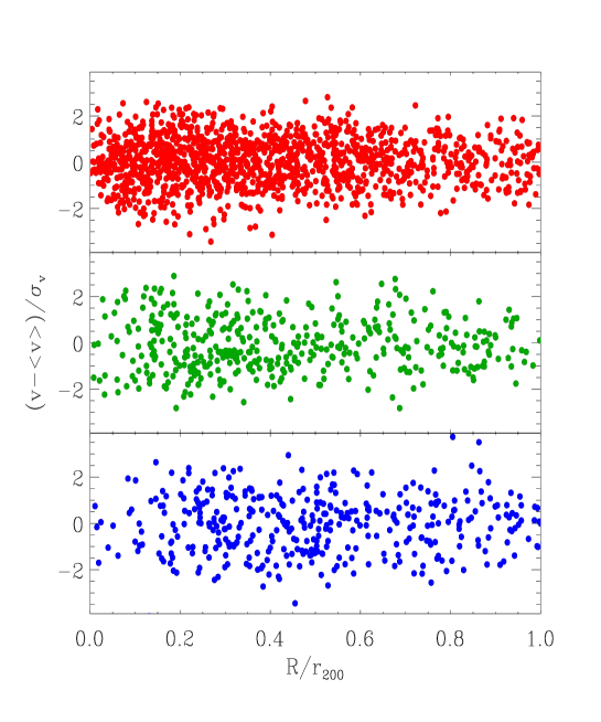
Figure 12: The projected phase-space distributions of different galaxy populations in ENACS clusters. Top panel: Es and S0s; middle panel: early-type S; bottom panel: late-type S and Irr. Galaxy clustercentric distances have been scaled with the cluster virial radii, and galaxy velocities relative to their cluster mean velocities have been scaled with the cluster velocity dispersions, in order to stack 59 cluster samples together. Galaxies in subclusters have been removed from the sample. From [99].

The most striking characteristics of the cluster galaxy population is its morphology mix. Nearby clusters contain a larger fraction of ETGs than of LTGs, exactly the opposite of what is observed in the general field. The morphological difference is so striking that it was noted even before the extragalactic nature of nebulae was established (see, e.g., [1]). Today, a modern version of the relation between galaxy properties and their environments is expressed by the segregation of different cluster galaxy populations in projected phase-space (see Fig. 12). ETGs populate higher-density cluster regions than LTGs, which are also characterized by a larger $\sigma_{v}$ at all radii. The very bright ellipticals (Es) occupy denser and lower-velocity regions than any other cluster galaxy population. Within the LTG population, the projected phase-space distribution of early-type spirals (Sa–Sb) is more similar to that of the ETGs than to that of late-type spirals and irregulars (Irr). Finally, galaxies in substructures appear to be avoiding the cluster centers and to move at relatively low velocities.

Why do galaxies care about their environment? Why different populations of galaxies occupy different regions of the phase-space? By analyzing the properties of galaxies as a function of their environment and of redshift it is possible to constrain the mechanisms of galaxy formation and evolution (see, e.g., [306]). Hereafter, the observational properties of galaxies in and around clusters, as a function of their environment and redshift are presented. Physical processes capable of shaping galaxy properties in clusters are then reviewed. Finally, an evolutionary scenario based on the observational phenomenology is proposed.

3.1 Morphology

The galaxy morphology mix changes with some regularity over many decades of projected galaxy number density, the fractions of Es and S0s increase with increasing local density and the fractions of S and Irr decrease [307, 308]. This is the so-called “morphology–density relation” (MDR in the following). Given the strong anti-correlation between local density and clustercentric distance (radius), the MDR is often reported as a variation of the morphological fractions with radius (see, e.g., [309]).

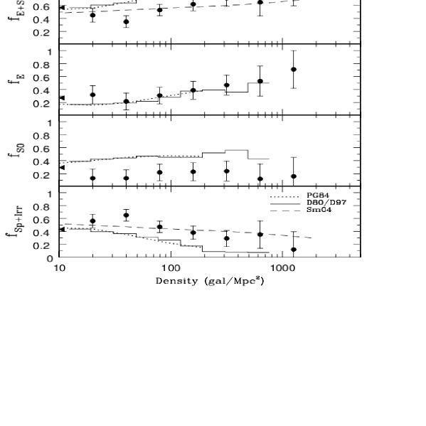
Figure 13: The MDR for $z\sim 1$ clusters (circles with error bars from [312], dashed line from [313]) compared with the same relation in local clusters (solid line from [307, 314], dotted line from [308]). From [312].

A less strong correlation exists between the morphologies and the velocities of cluster galaxies, Es and S0s having a narrower velocity distribution than S and Irr ([310, 193, 239, 311]; see also [1] and references therein). The MDR and the morphology–velocity relation together can be viewed as a segregation of different cluster galaxy populations in projected phase-space [99].

The MDR is present at least up to $z\sim 1$ in massive clusters [312, 313], while in low-mass, irregular clusters at $z\sim 0.5$ there is no evidence of the MDR [314]. The MDR is anyway evolving also in massive clusters, as the ETG fraction ($f_{ETG}$) decreases from $z\sim 0$ to $z\sim 1$ [314, 315, 316, 312, 313] (see Fig. 13). The observed $f_{ETG}$ evolution does not concern Es, which seem to be in place in the cluster environment well before $z>1$, but S0s, or rotationally supported spheroidals [317], whose fraction increases with decreasing $z$ at the expense of S and Irr in the highest density regions. The S0 fraction is $0.46\pm 0.06$ in local clusters, and decreases by a factor $\sim 2$ in $z\sim 1$ clusters [312]. In $z\sim 1$ clusters, S0s are $\sim 0.5$ Gyr younger than Es of similar luminosities [318]. Most of the S0 fraction evolution occurs at $z\leq 0.5$ [319] and concerns low-luminosity galaxies [320].

3.2 Colors

Most cluster galaxies are distributed in a narrow band in a color vs. magnitude diagram, the so-called color-magnitude relation, CMR hereafter [321, 322, 323]. In nearby groups and clusters the CMR is defined all the way down to dwarf galaxies [324, 325, 326]. The CMR is well defined also in high-$z$ clusters [327, 61, 318] and even for $z\approx 2$ protoclusters, but not so much for $z\approx 3$ protoclusters [328]. The mean color of the CMR galaxies indicates their stellar populations were formed at $z\geq 2.5$ [329, 330, 331].

The CMR is rather tight in nearby clusters, but its mean color and scatter increase with clustercentric distance and decreasing local density [332, 333, 334, 335] and at the fainter end of the LF [336]. The increased scatter suggests a younger average stellar population for the CMR galaxies in lower density regions, with an age gradient of 2.5 Gyr from the cluster center to its outskirts [334]. A smaller age gradient is also seen in high-$z$ clusters [318]. Spectral analyses show the field ETGs to be $\sim 1$ Gyr older than their cluster counterparts [337].

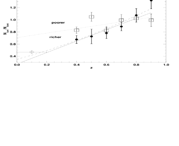
Figure 14: The ratio of luminous-to-faint CMR galaxies as a function of redshift, shown separately for richer (circles) and poorer (squares) clusters. A low-$z$ reference is also shown (diamond). From [338].

The CMR faint-end becomes less populated in high-$z$ clusters [339, 340, 331, 341] and this evolution occurs at different epochs depending on the cluster richness [338] (see Fig. 14). Hence the faint-end of the red cluster galaxy LF flattens [342, 343], and the dwarf-to-giant red-galaxy number-ratio decreases [344, 345, 346], with increasing $z$. As the number of faint red cluster galaxies diminishes with $z$, the number of blue cluster galaxies increases [338]. Such variations of the CMR with magnitude and $z$ are however not seen in all clusters [347, 348, 327], and this indicates that there is a significant cosmic variance in the evolution of cluster galaxy properties [334].

The $z$-evolution of the CMR was already noticed 30 years ago by Butcher & Oemler [349, 350]. They measured the red-galaxy fractions in two $z\simeq 0.4$ clusters, and found them to be significantly lower than in nearby clusters. This phenomenology has since been known as the Butcher-Oemler effect (BOe hereafter). The BOe can also be seen as an increase of the clustering strength of blue galaxies with increasing $z$ [351]. The BOe was initially suspected of being caused by field galaxies contamination, but spectroscopic observations have later confirmed the physical reality of the effect. As the fraction of blue cluster galaxies increases with $z$, also the fraction of galaxies with spectra characteristics of a young stellar population (e.g. the E+A galaxies) increases [353, 354, 355], a phenomenology known as the spectroscopic BOe. IR observations have discovered a population of IR-bright emitters in medium-$z$ clusters, not seen in nearby clusters [356, 357, 358, 359, 360, 361, 362], a phenomenology known as the IR-BOe. The BOe is stronger for fainter galaxies [363, 364] and in the more external parts of galaxy clusters [365, 195].

Altogether, studies of the CMR and BOe indicate that the color evolution of cluster galaxies occurs later for fainter galaxies, in lower-density regions, and in less massive clusters. The analyses of the MDR find exactly the same trends for the morphological evolution of cluster galaxies. Since there is a clear correlation between galaxy morphology and color, the obvious question is whether the morphology and color environmental dependences describe in fact the same physical phenomenon. There is evidence that galaxies in low-$z$ clusters do not show any MDR at fixed age (as deduced from their spectral energy distributions), suggesting the MDR is in fact an age–density relation [366]. Similarly, the MDR of galaxies in $0.4\leq z\leq 0.8$ clusters can be derived from the SF–density relation (which is strictly related to the age–density relation) by using the average SF per morphological class [367]. On the other hand, the radial increase of the CMR scatter has been shown to be too strong to be entirely accounted for by the MDR [333]. Hence the relation between galaxy colors and environment seems to be more fundamental than the MDR.

Morphological and color evolution do not seem however to proceed at the same speed. Morphological evolution seems to take longer than color evolution. This is indicated by the analysis of the evolution of the galaxy mass function [368], by the presence of passive, red cluster galaxies with spiral morphologies [369, 355, 370], and by the presence of early-type S which have the same age of S0s in the highest-density cluster regions [366].

3.3 Masses

The masses of cluster ETGs can be inferred from the analysis of the ETG fundamental plane (FP), a relation between the ETG internal velocity dispersions, their effective radii, and their effective brightnesses [371, 372, 373]. By studying the FP as a function of $z$, and based on spectrophotometric models, it is possible to constrain the ETG $M/L$ evolution, their average formation redshift ($z_{f}$), and the evolutionary history of their stellar populations [374]. FP studies indicate $z_{f}\geq 2$ for the most massive cluster ETGs, but more recent $M/L$ evolution and younger ages for ETGs of lower-masses [374, 375, 376, 377]. These studies also indicate that cluster ETGs are $\sim 0.4$ Gyr older than field ETGs [378], and that this age-difference increases with galaxy mass [375]. The $M/L$ of S0s and E+A galaxies are different from the $M/L$ of Es [379, 374], and this indicates that the former have experienced more recent episodes of SF.

Overall, the results obtained from the study of the FP support the conclusions reached from the studies of the CMR and MDR.

3.4 Luminosities

Many analyses have shown the LF of group and cluster galaxies to be different from the LF of field galaxies. In particular, compared to the LF of field galaxies, the LF of cluster galaxies is characterized by a steeper faint-end slope [380, 381, 83, 382, 383, 384, 385, 364, 386, 387, 388, 389, 390, 391, 392, 393], a brighter characteristic magnitude [394, 395, 396, 397], and a dip or plateau at intermediate luminosities [398, 380, 399, 400, 388] (see Fig. 15). According to other studies, however, there is no significant difference between the LF of cluster and field galaxies [401, 402, 403, 118, 404, 326, 405].

Different conclusions about the shape of the average LF of cluster galaxies may be reached if different clusters are characterized by different LFs, or if different studies consider different cluster regions and the LF changes with radius. While the cluster LF appears to be universal (see, e.g., [388]), there is evidence that its shape does change with radius, its faint-end slope being shallower (and hence similar to the field LF) in the central regions of clusters [83, 382, 406, 384, 407, 408, 409, 410, 386, 411, 388, 393]. It is also possible that the reported faint-end slopes of cluster LFs are overestimated because of incorrect field-count subtractions [412, 324, 393], or, vice versa, underestimated because of a biased selection against low surface-brightness galaxies [413].

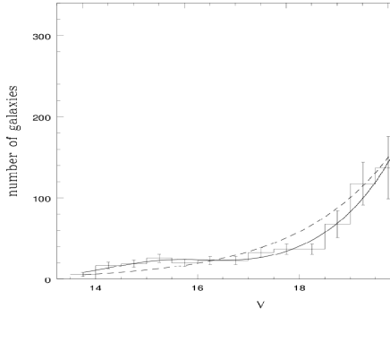
Figure 15: The LF of the Coma cluster of galaxies, showing the excess of bright galaxies relative to a Schechter function (dashed line), a steep faint-end upturn and a plateau at intermediate luminosities. The solid line is a Gaussian+Schechter fit to the data. From [83].

The ratio between the number of bright (giant) and of faint (dwarf) galaxies increases towards the cluster center, an effect known as luminosity segregation [1, 414]. Very bright cluster galaxies not only prefer the central regions, but are also closer to the mean cluster velocity, their $\sigma_{v}$ being only $\leq 1/2$ the global cluster $\sigma_{v}$ [201, 311]. Luminosity segregation is also found outside clusters (e.g. [415, 416]).

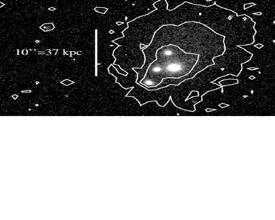
Figure 16: The central region of a $z=0.39$ X-ray selected galaxy cluster. Three companion galaxies are seen close to the BCG. Contours show $r$-band surface brightness levels and emphasize the presence of the ICL. Given the positions and velocities of the four galaxies, two of the companions are estimated to merge with the BCG in $\sim 0.1$ Gyr. From [428].

Two other characteristics distinguish the luminosity content of clusters from the field, the presence of BCGs and of the intra-cluster diffuse light (ICL in the following). BCGs are quite different from field ETGs of the same luminosities, in particular since their sizes are bigger [417, 418]. Moreover, BCGs are intimately related to their hosting cluster. In fact they live close to the bottom of the cluster potential [419, 267], their luminosities are correlated with the cluster total luminosities and masses [420], and their main axes are aligned along the main cluster axes [421].

There is evidence of some ongoing SF activity in many BCGs, probably activated by the cooling of the intra-cluster gas [422, 423], but overall the average color of the BCG stellar populations suggests they formed at $z\geq 2$ [424], and the total $K$-band luminosity of massive cluster BCGs evolves passively with $z$. On the other hand, BCGs in clusters of low masses do show substantial stellar mass evolution, with a factor 2–4 increase in mass since $z\sim 1$ [425, 426]. This is consistent with the fact that the fractional cluster luminosity in the BCG is anti-correlated with the total cluster light [420], as if BCGs in massive clusters completed their assembly before their counterparts in low-mass clusters.

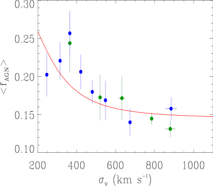
Figure 17: The AGN fraction as a function of the galaxy system velocity dispersion for two samples. The solid line is a model based on a galaxy merging-rate relation [459]. From [442].

Support for the hypothesis that at least some cluster BCGs have yet to complete their assembly comes from the observation that the luminosity ratio between the BCG and the second-ranked cluster galaxy is smaller for the less massive and irregular clusters [427, 267]. Direct evidence for ongoing build-up of BCGs in some $z\simeq 0.4$ clusters and groups has also been provided [428, 429] (see Fig. 16).

The amount of ICL in groups and clusters is not very well constrained. It is estimated to be $\sim 5$–25% of the total cluster light [430, 431, 432, 433, 434, 435], and as much as 50% near cluster centers [436]. The properties of the BCGs and the ICL are related, suggesting a direct, physical link. Their colors and elongation axes are in fact similar, and clusters with brighter BCGs have higher ICL surface brightnesses [437].

3.5 Nuclear activity

There is observational evidence that the fraction of active galactic nuclei ($f_{AGN}$) is higher in galaxy pairs [438] and in compact groups [439], and lower in clusters [353], relative to isolated field galaxies. However, other studies have found no environmental dependence of $f_{AGN}$ [440, 441].

The striking difference between $f_{AGN}$ in compact groups and in clusters suggests it is not the density of the environment that matters for the onset of the AGN activity. In fact, galaxy number densities in compact groups and clusters are both very high. On the other hand, cluster $\sigma_{v}$s are typically $\sim 3$ times larger than those of compact groups. Hence, the onset of AGN activity may depend more on the relative galaxy velocities, than on galaxy density. A study of several hundred groups and clusters has indeed shown that $f_{AGN}$ is anti-correlated with the velocity dispersion of the host galaxy system [442] (see Fig. 17).

3.6 Physical processes

Several physical processes are capable of affecting the properties of cluster (and group) galaxies. They result from the interactions among galaxies, with the cluster gravitational potential, and with the intra-cluster medium [443]. The most important of these processes are the following:

• dynamical friction [146, 444];

• galaxy-galaxy collisions [445, 446], leading to tidal effects and, eventually, mergers [447, 448];

• tidal forces induced by the cluster gravitational potential, resulting in tidal truncation of the galactic halos [449, 450, 237];

• ram-pressure stripping of the galaxy gas [451, 452].

Dynamical friction is the process that slows down a massive galaxy as it moves in a sea of dark matter particles. These particles are gravitationally focused in the wake of the galaxy itself. The galaxy therefore feels a braking force resulting from the excess mass density of the dark matter particles in the direction opposite to its motion. The characteristic timescale of this process is

$$t_{df}\propto\frac{v_{g}^{3}}{m_{g}\rho},$$ (17)

where $v_{g}$ is the galaxy velocity, $m_{g}$ its mass, and $\rho$ is the dark matter density [146, 453]. Hence dynamical friction is more effective in higher density environments and for more massive galaxies and not very effective when the galaxy moves fast.

Collisions and mergers drive substantial galaxy morphological modifications [448, 454], and induce starburst episodes in the central galaxy regions [455, 456, 457], which then consume the available gas content. Gas can also be expelled from the galaxies as these collide and eventually merge [448, 458], since the total mass of the merger product is generally less than the sum of the progenitor masses. The characteristic timescale for a galaxy to experience a collision with another galaxy is

$$t_{c}\propto\frac{1}{\nu r_{g}^{2}v_{g}},$$ (18)

where $v_{g}$ is the relative velocity between the two galaxies, $r_{g}$ the galaxy radius, and $\nu$ is the galaxy number density [277]. Hence collisions happen more frequently in higher density environments and between larger galaxies.

The impulsive tidal field produced by the collision produces collisional stripping [450]. This is most important for the material in the external regions of non-compact galaxies undergoing close encounters, since the tidal force is proportional to $r_{g}/d^{3}$, where $d$ is the distance to the colliding galaxy.

Galaxy-galaxy collisions may lead to mergers when the relative speed of the encounter is very low. The characteristic timescale for a merger to occur is

$$t_{m}\propto\frac{\sigma_{v}^{3}}{\nu r_{g}^{2}\sigma_{g}^{4}},$$ (19)

where $\sigma_{v}$ is the cluster velocity dispersion and $\sigma_{g}$ is the internal velocity dispersion of the galaxy [459, 460]. Mergers are therefore very effective in low-velocity dispersion, high-density environments, such as groups and cluster outskirts (filaments).

A galaxy moving on a circular orbit in the core of a cluster with core radius $r_{c}$ will suffer tidal truncation of its external parts, beyond a radius [450]

$$r_{t}\approx r_{c}\frac{\sigma_{g}}{2\sigma_{v}}.$$ (20)

Hence galaxies moving in massive and centrally concentrated clusters will be severely truncated, and their external (dark matter and gaseous) halos will become part of the intra-cluster matter as they come close to the cluster center [237]. Note however that galaxies sitting at the bottom of the cluster potential, i.e. BCGs, are not truncated by this mechanism since they feel symmetric external forces. Eq. (20) may however not be applicable to field galaxies entering the cluster along filaments, since their orbits are mildly radially anisotropic, and not circular [237, 226]. For these more general orbits, numerical simulations indicate that eq. (20) is still valid, once $r_{c}/2$ is replaced with the radius of the orbit pericenter [237, 461].

The tidal forces induced by the cluster potential also lead to the compression of galactic gas and can therefore stimulate SF [462, 457].

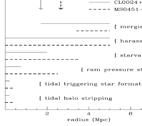
Figure 18: This diagram indicates the clustercentric radius over which the listed mechanisms are effective in shaping galaxy properties. Two clusters are considered, with $M_{200}$ masses $\simeq 9$ and $\simeq 14$ in units of $10^{14}M_{\odot}$ (Cl0024+17 and MS0451-03, respectively). Arrows indicate the cluster virial radii. The indicated tidal processes refer to interactions with the cluster potential, while the term “harassment” refers to the effect of galaxy-galaxy collisions. From [373].

A galaxy moving in a cluster will feel a pressure exerted by the intra-cluster diffuse gas onto the gas of its disk and the gas reservoir in its halo. The disk gas will be stripped under the condition that the ram pressure of the intra-cluster gas exceeds the gravitational restoring force per unit area on the disk,

$$\rho_{IC}v_{g}^{2}>2\pi G\Sigma_{\star}\Sigma_{gas},$$ (21)

where $\rho_{IC}$ is the intra-cluster gas density, and $\Sigma_{\star}$ and $\Sigma_{gas}$ are the stellar and gaseous surface densities of the disk, respectively [451, 463]. In fact, eq. (21) is strictly valid only if the baryons dominate the mass budget of the galaxy disk. As far as the gas in the galaxy halo is concerned, the stripping condition can be written as follows

$$\rho_{IC}v_{g}^{2}>\alpha\frac{Gm_{g}\rho_{gas}}{R_{g}},$$ (22)

where $R_{g}$ is the projected galaxy radius in the direction transverse to the galaxy motion, $\rho_{gas}$ is the 3-d galaxy gas-density profile and the $\alpha$ term, of order unity, depends on the precise shape of the gas and mass profiles of the galaxy [463]. From eqs. (21) and (22) it is clear that it is easier to strip the gas from a lower-mass galaxy moving at higher speed in a denser intra-cluster medium.

Ram-pressure, tidal truncation, collisional stripping can all lead to starvation [464, 465]. Present-day spirals would use their disk gas content in a few Gyr at their current SF rates. If these SF rates must be sustained over a Hubble time, the disks must be refueled by gas reservoirs in galaxy halos. Starvation results from removing the gas reservoir.

It is important to note that the effectiveness of the different processes depend on the clustercentric distances and on the cluster masses. E.g. merging will operate more effectively in the cluster outskirts and for lower-mass clusters, and ram-pressure stripping in the cluster inner regions and for higher-mass clusters (see Fig. 18).

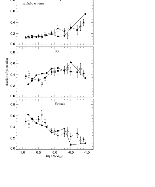
Figure 19: The morphological mix of galaxies as a function of clustercentric radius in simulations (dashed line; filled and open squares correspond to bright and faint galaxies) as compared to real data (solid line, from [309]). The agreement is excellent but the definition of ’numerical S0s’ has been widened to include ’numerical early-spirals’, otherwise a deficit of S0s compared to the observational sample would have resulted. From [166].

3.7 A scenario for the evolution of galaxies in clusters

What makes the properties of cluster galaxies differ from those of field galaxies? Do galaxies change their colors, morphologies, luminosities, and even nuclear activities, as they move from regions of lower density to regions of higher density under the influence of gravity? Or are galaxy properties established once and for ever since their formation? The two scenarios confront each other, but are not necessarily mutually exclusive.

Several characteristics of the cluster galaxy population argue in favor of the scenario in which galaxy properties are established ab initio. In particular, both the CMR and the MDR seem to be established already in $z\geq 1$ clusters, and the color and FP-inferred $M/L$-evolution of bright cluster ETGs indicate simple passive evolution since $z_{f}\geq 2$. However, other observations argue for a modification of the galaxy properties with time. In particular, there is a deficit of both faint ETGs and S0s in high-$z$ clusters, as indicated by studies of the CMR, the MDR and the LF. This deficit is more conspicuous for less massive and more irregular clusters. The analyses of the CMR, the FP, and the ETG spectra also show that the average age of the ETG stellar population increases with the local density.

A natural expectation of hierarchical cosmological models is biased galaxy formation (e.g. [466]), galaxies in denser environments form earlier, and are more massive than those formed later, because they form with an initially larger mass and undergo more mergers during their lifetime. These models are able to approximately reproduce the environmental dependences of galaxy properties [467, 166, 468, 469, 470] (see Fig. 19). Mergers increase the masses of galaxies, destroy spiral features and disks, reduce angular momentum. They also trigger a starburst that consumes part of the available galaxy gas. Mergers are therefore effective in driving a LTG to ETG transition.

A merger can also form and/or activate a central black hole, hence an AGN, perhaps with a certain delay after the starburst [471]. This is observationally supported by the fact that AGN host galaxies have colors and morphologies suggestive of a 1–4 Gyr old starburst associated with a merger event [472], and by the fact that a merger model fits the relation between $f_{AGN}$ and $\sigma_{v}$ of galaxy systems [442]. The resulting AGN feedback could quench any remaining SF activity [473, 474], more strongly so in more massive galaxies, characterized by larger black hole masses [475]. The AGN energy output into the intra-group medium can also explain the phenomenology of group X-ray scaling relations [476].

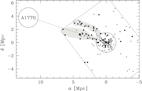
Figure 20: Spatial distribution of members of the A1763 galaxy cluster at $z\sim 0.2$. Starburst galaxies identified by their IR emission are indicated with filled dots. The triangle indicates an AGN. Circles of 1.5 Mpc are drawn around the central positions of A1763 and its neighbor A1770. Shaded regions highlight the kinematically-detected filaments, where most starburst galaxies are located [482].

Mergers of small galaxies or galaxy subunits should be able to form red Es at the cluster centers at times when cluster $\sigma_{v}$s have not yet become too high. A merger origin of cluster Es is indeed suggested by their flat metallicity and color gradients [477, 478]. Mergers become inefficient at later times in high density regions, when these become characterized by high values of $\sigma_{v}$ (see eq. 19). But mergers can still operate in lower-density regions. Hence, low-density regions should be populated by galaxies forming at later times, and hence grown up to smaller masses, in agreement with the observed trends of galaxy age with density and radius inferred from the analyses of the CMR relation. At intermediate $z$, the IR-BOe is suggestive of mergers among galaxies located in medium-density environments but outside the highest-density cluster regions [479]. At lower $z$, the merger activity is restricted to galaxies outside the cluster virial regions, as indicated by the high fraction of starburst galaxies detected in the relatively high-density, but low-$\sigma_{v}$ cluster-feeding filaments [480, 481, 482] (see Fig. 20). Most of these starburst galaxies have small stellar masses.

Summing up, high-density regions are the birthplace of massive galaxies, which assembly most of their mass at early times, before mergers become inefficient. Mergers stimulate SF and AGNs that successively quench any further SF. In lower-density environments less massive galaxies are formed, and the formation process is delayed. SF hence stops earlier in more massive galaxies in higher-density environments. At least qualitatively, this scenario is consistent with the observation that the critical mass above which SF is suppressed increases with $z$, and more rapidly in denser environments [483, 368], the so-called “downsizing” effect [484].

According to numerical simulations, mergers of cluster galaxies can also make BCGs [485, 301]. Support for a merger origin of BCGs comes from their shallow surface-brightness profiles [486]. BCG assembly can continue until very late, and is only $\sim 50$% finished by $z\sim 0.5$ [301]. Direct observational evidence that BCGs continue their mass growth at $z<0.5$ has recently been provided [428, 429]. The more recent mass evolution of BCGs in lower-mass clusters [425, 426] is just another manifestation of the downsizing process. Cluster $\sigma_{v}$s would generally be too high for BCGs to continue growing at recent times, even in relatively low-mass clusters, but dynamical friction can decrease the relative velocities of the more massive cluster galaxies orbiting the cluster central regions. Velocity segregation of the most luminous cluster galaxies is indeed observed [201] and is also predicted by numerical simulations [166]. Dynamical friction and mergers of the brightest galaxies in the central regions of galaxy systems can also account for the intermediate-luminosity dip and the brighter characteristic luminosity of the cluster LF, relative to the field LF [487, 488, 489].

Galaxy mergers must also be important in the formation of the ICL. The ICL characteristics are clearly related to the characteristics of the BCG, suggesting their common origin. The product of galaxy mergers is unlikely to contain 100% of the mass of their progenitors, as part of the stars of the initial galaxies are scattered away during the galaxy-galaxy collision. If $\sim 1/3$ of the stars of the merging galaxies are scattered into the ICL component at each merger event, it is possible to reconcile current hierarchical cosmological models with the lack of evolution since $z\sim 1$ of the stellar mass function at the high-mass end [490, 491, 492]. Numerical simulations predict that if the ICL is built through galaxy-galaxy collisions its fractional contribution to the total cluster light should be almost independent on cluster mass [493], a prediction consistent with some observational estimates [494], and in contrast with others [495]. Anyway, direct evidence for the ICL creation through galaxy-galaxy collisions comes from observations of compact groups [496]. Dwarf galaxies can form in the tidal tails of galaxy-galaxy collisions [497] contributing to steepen the LF faint-end of galaxy clusters. These tidal dwarfs are then rapidly destroyed in high-density regions by collisions with other galaxies, thus explaining why a flatter LF characterizes cluster central regions.

Mergers and dynamical friction are therefore important processes in the evolution of cluster and group galaxies. On the other hand, the abundance of S0 galaxies in clusters and its late-evolution are more difficult to explain [467, 166, 468]. Low-luminosity S0s could form from spirals through the fading of the spiral disks resulting from gas removal (starvation) [498, 373]. The production of S0s from spirals is suggested by the relative evolution of the LFs of blue and red galaxies [338] and by the presence of a cluster galaxy population intermediate between ETGs and LTGs, the population of passively-evolving galaxies with spiral arms and red disks [499, 373]. These passive spirals are generally also characterized by a very low-HI gas content given their stellar mass or luminosity (see, e.g., [500, 501]). The formation of S0s via the fading of spiral disks is also suggested by the analyses of the Tully-Fisher relation and the globular cluster fraction of cluster S0s [502, 503, 504], as well as by the smaller disk sizes of cluster spirals relative to field spirals [505, 506].

The precise mechanism by which cluster spirals loose their gas can vary, both with the mass of the accreting cluster, and with the distance from the cluster center [507, 373]. In the central regions of massive clusters, ram-pressure stripping is expected to be the dominant mechanism [508], but tidal shocks in the cluster potential can also be important if the cluster mass distribution is highly concentrated [509]. At larger radii, and in low-mass clusters and groups, galaxy-galaxy collisions and related tidal stripping should dominate [306, 510, 511]. These collisions can produce central bursts of SF, accelerating the disk gas consumption. There is indeed conspicuous observational evidence that at least some cluster (or group) S0s have experienced recent episodes of SF [512, 498, 513, 330, 514, 373, 515, 516]. If processes operating in the cluster outskirts are effective enough in removing the gas of infalling field spirals, processes operating near the cluster center may play little rôle in the evolution of cluster galaxies [306, 517, 469].

The fading of spiral disks reduces galaxy luminosities by $\geq 1$ mag, hence it is impossible to form bright S0s by this mechanism. In order to produce bright S0s from spirals, the spiral bulge mass must increase. This can occur by a central burst of SF [517] induced by minor mergers [518, 519] and/or major tidal heating. The tidal heating can be caused by galaxy-galaxy collisions or by the gradient of the cluster gravitational potential [277]. When galaxies collide at high speed, no merger can occur and tidal damage is limited, hence bright cluster S0s can only form at high-$z$ before the cluster $\sigma_{v}$ becomes too large. At low-$z$, bright S0s can form in small, low-$\sigma_{v}$ groups. As these groups are accreted by clusters, they then become part of the cluster galaxy population [488, 443, 520]. Accreted groups are identified as subclusters, and an excess of S0s in subclusters in the central regions of nearby clusters has indeed been observed [99].

Possible progenitors of the bright S0s are early-type spirals (Se). In fact, the bulge luminosities of Se are comparable to those of S0s [521], Se and S0s occupy regions of similar (albeit somewhat lower) local densities [522], the stellar populations of the Se and S0s that reside in high density environments have similar ages [366], and Se and S0s move on similar, nearly-isotropic, orbits [226]. Other plausible progenitors of the bright S0s are the E+A galaxies. Spectrophotometric modeling indicates that E+A cluster galaxies should passively evolve into bright S0s [523]. E+A galaxies have positive color gradients [524] and have close companions and/or tidal features indicative of interactions [525], all features consistent with a merger origin of these galaxies. Recently, a population of dusty starburst galaxies, bright enough to evolve into bright S0s after the SF episode has ceased, has been identified in $z\sim 0.5$ clusters, using observations with the Spitzer satellite [360, 361]. Many of these presumed S0-progenitors are found to reside in subclusters, where the galaxies can collide at relatively low speeds.

Albeit very sketchy, the scenario outlined above tries to account for a large part (if not all) of the observational evidences of the environmental dependence of galaxy properties as a function of $z$. With a precise theory of galaxy formation and evolution yet to be formulated, and an infinity of data yet to be collected, our current (rather modest) understanding of galaxy evolution in clusters will certainly have to be revised in the near future.

- [1] \BYBiviano A. in Constructing the Universe with Clusters of Galaxies, edited by , F. Durret and D. Gerbal, 2000, http://nedwww.ipac.caltech.edu/level5/Biviano2/frames.html, astro-ph/0010409
- [2] \BYAbell G.O. \INApJS31958211
- [3] \BYAbell G.O., Corwin H.G.Jr., \atqueOlowin R.P. \INApJS7019891
- [4] \BYKatgert P., Mazure A., Perea J. et al. \INA&A310199630
- [5] \BYKatgert P., Mazure A., den Hartog R. et al. \INA&AS1291998399
- [6] \BYLucey J.R. \INMNRAS204198333
- [7] \BYBriel U.G. \atqueHenry J.P. \INA&A2781993379
- [8] \BYGal R.R., de Carvalho R.R., Lopes P.A.A. et al. \INAJ12520032064
- [9] \BYKoester B.P., McKay T.A., Annis J. et al. \INApJ6602007221
- [10] \BYPostman M., Lubin L.M., Gunn J.E. et al. \INAJ1111996615
- [11] \BYKepner J., Fan X., Bahcall N. et al. \INApJ517199978
- [12] \BYLobo C., Iovino A., Lazzati D. \atqueChincarini G. \INA&A3602000896
- [13] \BYDong F., Pierpaoli E., Gunn J.E. \atqueWechsler R.H. \INApJ6762008868
- [14] \BYHuchra J.P. \atqueGeller M.J. \INApJ2571982423
- [15] \BYGeller M.J. \atqueHuchra J.P. \INApJS52198361
- [16] \BYRamella M., Geller M.J. \atqueHuchra J.P. \INApJ344198957
- [17] \BYEke V.R., Baugh C.M., Cole S. et al. \INMNRAS3482004866
- [18] \BYBerlind A.A., Frieman J., Weinberg D.H. et al. \INApJS167(2006)1
- [19] \BYvan Breukelen C., Clewley L., Bonfield D.G. et al. \INMNRAS3732006L26
- [20] \BYOlsen L.F., Scodeggio M., da Costa L. et al. \INA&A3451999681
- [21] \BYBahcall N.A., McKay T., Annis J. et al. \INApJS1482003243
- [22] \BYKochanek C.S., White M., Hucra J. et al. \INApJ5852003161
- [23] \BYWillick J.A., Thompson K.L., Mathiesen B.F. et al. \INPASP1132001658
- [24] \BYDonahue M., Scharf C.A., Mack J. et al. \INApJ5692002689
- [25] \BYPostman M, Lauer T., Oegerle W. \atqueDonahue M. \INApJ579200293
- [26] \BYDietrich J.P., Erben T., Lamer G. et al. \INA&A4702007821
- [27] \BYBenoist C., da Costa L., Jørgensen H.E. et al. \INA&A39420021
- [28] \BYOlsen L.F., Zucca E., Bardelli S. et al. \INA&A4422005841
- [29] \BYBasilakos S., Plionis M., Georgakakis A et al. \INMNRAS3512004989
- [30] \BYBower R.G., Castander F.J., Couch W.J., Ellis R.S. \atqueBöhringer H. \INMNRAS2911997353
- [31] \BYMcNamara B.R., Vikhlinin A., Hornstrup A. et al. \INApJ5582001590
- [32] \BYPopesso P., Biviano A., Böhringer H. \atqueRomaniello M. \INA&A4612007397
- [33] \BYSchuecker P., Böhringer H., \atqueVoges W. \INA&A420200461
- [34] \BYRamella M., Pisani A., \atqueGeller M.J. \INAJ1131997483
- [35] \BYMaia M.A.G., da Costa L.N., \atqueLatham D.N. \INApJS691989809
- [36] \BYTucker D.L., Oemler A.Jr., Hashimoto Y. et al. \INApJS1302000237
- [37] \BYRamella M., Zamorani G., Zucca E. et al. \INA&A34219991
- [38] \BYMerchán M.E. \atqueZandivarez A. \INApJ6302005759
- [39] \BYCrook A.C., Huchra J.P., Martimbeau N. et al. \INApJ6552007790
- [40] \BYDeng X.-F., He J.-Z., Jiang P., Luo C.-H., \atqueWu P. \INA&A474(2007)783
- [41] \BYTago E., Einasto J., Saar E. et al. \INA&A4792008927
- [42] \BYCarlberg R.G., Yee H.K.C., Morris S.L. et al. \INApJ5522001427
- [43] \BYYang X., Mo H.J., van den Bosch F.C., \atqueJing Y.P. \INMNRAS35620051293
- [44] \BYWeinmann S.M., van den Bosch F.C., Yang X., \atqueMo H.J. \INMNRAS36620062
- [45] \BYGladders M.D. \atqueYee H.K.C. \INAJ12020002148
- [46] \BYGladders M.D. \atqueYee H.K.C. \INApJS15720051
- [47] \BYCohn J.D., Evrard A.E., White M., Croton D. \atqueEllingson E. \INMNRAS38220071738
- [48] \BYGladders M.D., Yee H.K.C., Majumdar S. et al. \INApJ6552007128
- [49] \BYBarrientos L.F., Gladders M.D., Yee H.K.C. et al. \INApJ6172004L17
- [50] \BYEisenhardt P.R.M., Brodwin M., Gonzalez A.M. et al. \INApJ6842008905
- [51] \BYWilson G., Muzzin A., Lacy M. et al. in Infrared Diagnostics of Galaxy Evolution, edited by R.-R. Chary, H.I. Teplitz and K. Sheth, ASP Conf. Series, Vol.381 (2008) p.210
- [52] \BYPapovich C. \INApJ6762008206
- [53] \BYGoto T., Hanami H., Im M. et al. (2008) arXiv:0810.0529
- [54] \BYKoester B.P., McKay T.A., Annis J. et al. \INApJ6602007239
- [55] \BYGoto T., Sekiguchi M., Nichol R.C. et al. \INAJ12320021807
- [56] \BYMiller C.J., Nichol R.C., Reichart D. et al. \INAJ1302005968
- [57] \BYStanford S.A., Eisenhardt P.R., Brodwin M. et al. \INApJ6342005L129
- [58] \BYElston R.J., Gonzalez A.H., McKenzie E. et al. \INApJ6392006816
- [59] \BYBrodwin M., Eisenhardt P.R., Gonzalez A.H. et al. (2008) arXiv:0805.8013
- [60] \BYGilli R., Cimatti A., Daddi E. et al. \INApJ5922003721
- [61] \BYKurk J., Cimatti A., Zamorani G. et al. (2008) arXiv:0804.4126
- [62] \BYRamella M., Boschin W., Fadda D. \atqueNonino M. \INA&A3682001776
- [63] \BYBarrena R., Ramella M., Boschin W. et al. \INA&A4442005685
- [64] \BYKim R.S.J., Kepner J.V., Postman M. et al. \INAJ123200220
- [65] \BYBarkhouse W.A., Green P.J., Vikhlinin A. et al. \INApJ6452006955
- [66] \BYMarinoni C., Davis M., Newman J.A., \atqueCoil A.L. \INApJ5802002122
- [67] \BYGerke B.F., Newman J.A., Davis M. et al. \INApJ62520056
- [68] \BYGonzalez A.H., Zaritsky D., Dalcanton J. \atqueNelson A. \INApJS1372001117
- [69] \BYBartelmann M. \atqueWhite S.D.M. \INA&A3882002732
- [70] \BYGonzalez A.H., Zaritsky D., Simard L., Clowe D. \atqueWhite S.D.M. \INApJ5792002577
- [71] \BYWhite S.D.M., Clowe D.I., Simard L. et al. \INA&A4442005365
- [72] \BYAbell G.O. \INAJ661961607
- [73] \BYBahcall N.A. \atqueSoneira R.M. \INApJ277198427
- [74] \BYBatuski D.J. \atqueBurns J.O. \INAJ9019851413
- [75] \BYZucca E., Zamorani G., Scaramella R. \atqueVettolani G. \INApJ4071993470
- [76] \BYEinasto M., Tago E., Jaaniste J., Einasto J. \atqueAndernach H. \INA&AS1231997119
- [77] \BYKalinkov M \atqueKuneva I. \INA&AS1131995451
- [78] \BYEinasto J., Einasto M., Saar E. et al. \INA&A4592006L1
- [79] \BYEinasto J., Einasto M., Saar E. et al. \INA&A4622007811
- [80] \BYGott J.R.III, Melott A.L. \atqueDickinson M. \INApJ3061986341
- [81] \BYMecke K.R., Buchert T. \atqueWagner H. \INA&A2881994697
- [82] \BYBharadwaj S., Sahni V., Sathyaprakash B.S., Shandarin S.F \atqueYess C. \INApJ528200021
- [83] \BYLobo C., Biviano A., Durret F. et al. \INA&A3171997385
- [84] \BYSchechter P. \INApJ2031976297
- [85] \BYLin Y.-T., Mohr J.J. \atqueStanford S.A. \INApJ5912003741
- [86] \BYBinney J. \atqueTremaine S. Galactic Dynamics (Princeton: Princeton University Press) 1987
- [87] \BYNavarro J.F., Frenk C.S. \atqueWhite S.D.M. \INApJ4621996536
- [88] \BYMamon G.A. \atqueŁokas E.L. \INMNRAS3632005705
- [89] \BYYee H.K.C. \atqueEllingson E. \INApJ5852003215
- [90] \BYMuzzin A., Yee H.K.C., Hall P.B., \atqueLin H. \INApJ6632007150
- [91] \BYZwicky F. \INHelv. Phys. Acta6193310
- [92] \BYZwicky F. \INApJ861937217
- [93] \BYSmith S. \INApJ83193623
- [94] \BYLimber D.N. \atqueMathews W.G. \INApJ1321960286
- [95] \BYThe L.S. \atqueWhite S.D.M. \INAJ9219861248
- [96] \BYGirardi M., Giuricin G., Mardirossian F., Mezzetti M. \atqueBoschin W. \INApJ505199874
- [97] \BYBiviano A., Murante G., Borgani S. et al. \INA&A456200623
- [98] \BYMerritt D. \INApJ3131987121
- [99] \BYBiviano A., Katgert P., Thomas T., \atqueAdami C. \INA&A38720028
- [100] \BYBiviano A., Katgert P., Mazure A. et al. \INA&A321199784
- [101] \BYGill S.P.D., Knebe A., Gibson B.K., \atqueDopita M.A. \INMNRAS3512004410
- [102] \BYHicks A.K., Ellingson E., Hoekstra H. \atqueYee, H.K.C. \INApJ6522006232
- [103] \BYJohnson O., Best P., Zaritsky D. et al. \INMNRAS37120061777
- [104] \BYWu X.-P., Chiueh T., Fang L.-Z. \atqueXue Y.-J. \INMNRAS3011998861
- [105] \BYSmail I., Dressler A., Couch W.J. et al. \INApJ579199670
- [106] \BYWu X.-P., \atqueFang L.-Z. \INApJ483199762
- [107] \BYFinoguenov A., Reiprich T.H. \atqueBöhringer H. \INA&A3682001749
- [108] \BYEttori S., De Grandi S. \atqueMolendi S. \INA&A3912002841
- [109] \BYAndernach H., Plionis M., López-Cruz O., Tago E. \atqueBasilakos, S. in Nearby Large-Scale Structures and the Zone of Avoidance, edited by A.P. Fairall and P.A. Woudt, ASP Conf. Series, Vol.329 (2005) p.289
- [110] \BYPopesso P., Biviano A., Böhringer H., Romaniello M. \atqueVoges W. \INA&A4332005431
- [111] \BYCypriano E.S., Sodré L.Jr., Kneib J.-P., \atqueCampusano L.E. \INRMxAC262006111
- [112] \BYHashimoto Y., Henry J.P., Böhringer H. \atqueHasinger G. \INA&A468200725
- [113] \BYRines K., Diaferio A. \atqueNatarajan P. \INApJ6792008L1
- [114] \BYBorgani S., Rosati P., Tozzi P. et al. \INApJ561200113
- [115] \BYLopes P.A.A., de Carvalho R.R., Capelato, H.V. et al. \INApJ6482006209
- [116] \BYGirardi M., Manzato P., Mezzetti M., Giuricin G., \atqueLimboz F. \INApJ5692002720
- [117] \BYBahcall N.A., Dong F., Bode P. et al. \INApJ5852003182
- [118] \BYLin Y.-T., Mohr J.J., \atqueStanford S.A. \INApJ6102004745
- [119] \BYRamella M., Boschin W., Geller M.J., Mahdavi A., \atqueRines K. \INAJ12820042022
- [120] \BYBecker M.R., McKay T.A., Koester B. et al. \INApJ6692007905
- [121] \BYMuriel H., Quintana H., Infante L, Lambas D.G. \atqueWay M.J. \INAJ12420021934
- [122] \BYSchaeffer R., Maurogordato S., Cappi A. \atqueBernardeau F. \INMNRAS2631993L21
- [123] \BYAdami C., Mazure A., Biviano A., Katgert P. \atqueRhhe G. \INA&A3311998493
- [124] \BYRines K., Geller M.J., Diaferio A., Kurtz M.J. \atqueJarrett T.H. \INAJ12820041078
- [125] \BYPlionis M., Basilakos S. \atqueRagone-Figueroa C. \INApJ6502006770
- [126] \BYPopesso P., Biviano A., Böhringer H. \atqueRomaniello M. \INA&A4642007451
- [127] \BYMarinoni C. \atqueHudson M.J. \INApJ5692002101
- [128] \BYEke V.R, Frenk C.S., Baugh C.M. et al. \INMNRAS3552004769
- [129] \BYBrough S., Forbes D.A., Kilborn V.A. \atqueCouch W. \INMNRAS37020061223
- [130] \BYKauffmann G., Colberg J., Diaferio A. \atqueWhite S.D.M. \INMNRAS3031999188
- [131] \BYBenson A.J., Cole S., Frenk C.S. et al. \INMNRAS3112000793
- [132] \BYLin Y.-T., Mohr J.J., Gonzalez A.H. \atqueStanford S.A \INApJ6502006L99
- [133] \BYGilbank D.G., Yee H.K.C., Ellingson E. et al. \INAJ1342007282
- [134] \BYGilbank D.G., Yee H.K.C., Ellingson E. et al. \INApJ6772008L89
- [135] \BYGilbank D.G., Bower R.G., Castander F.J. \atqueZiegler B.L. \INMNRAS3482004551
- [136] \BYLubin L.M., Mulchaey J.S. \atquePostman M. \INApJ6012004L9
- [137] \BYFang T., Gerke B.F., Davis D.S. et al. \INApJ6602007L27
- [138] \BYHelsdon S.F. \atquePonman T.J. \INMNRAS3192000933
- [139] \BYOsmond J.P.F. \atquePonman T.J. \INMNRAS35020041511
- [140] \BYHelsdon S.F., Ponman T.J. \atqueMulchaey J.S. \INApJ6182005679
- [141] \BYValtchanov I., Pierre M., Willis J. et al. \INA&A423200475
- [142] \BYDai X., Kochanek C.S. \atqueMorgan N.D. \INApJ6582007917
- [143] \BYRykoff E.S., McKay T.A., Becker M.R. et al. \INApJ67520081106
- [144] \BYKocevski D.D., Lubin L.M., Gal R. et al. (2008) arXiv:0804.1955
- [145] \BYLedlow M., Voges W., Owen F.N. \atqueBurns J.O. \INAJ12620032740
- [146] \BYChandrasekhar S. \INApJ971943255
- [147] \BYTinker J.L., Weinberg D.H., Zheng Z. \atqueZehavi I. \INApJ631200541
- [148] \BYAbell G.O. \INARA&A319651
- [149] \BYBahcall N.A., Lubin L.M. \atqueDorman V. \INApJ4471995L81
- [150] \BYCarlberg R.G., Yee H.K., Ellingson E. et al. \INApJ462199632
- [151] \BYCarlberg R.G., Yee H.K. \atqueEllingson E. \INApJ4781997462
- [152] \BYAdami C., Mazure A., Katgert P. \atqueBiviano A. \INA&A336199863
- [153] \BYPress W.H. \atqueSchechter P. \INApJ1871974425
- [154] \BYSheth R.K. \atqueTormen G. \INMNRAS3081999119
- [155] \BYJenkins A., Frenk C.S., White S.D.M. et al. \INMNRAS3212001372
- [156] \BYBorgani S. \atqueGuzzo L. \INNature409200139
- [157] \BYEvrard A.E., MacFarland T.J., Couchman H.M.P. et al. \INApJ57320027
- [158] \BYDunkley J., Komatsu E., Nolta M.R. et al. (2008) arXiv:0803.0586
- [159] \BYEke V.R., Baugh C.M., Cole S., Frenk C.S., \atqueNavarro J.F. \INMNRAS37020061147
- [160] \BYSchuecker P., Böhringer H., Collins C.A., \atqueGuzzo L. \INA&A3982003867
- [161] \BYRasmussen J., Ponman T.J., Mulchaey J.S., Miles T.A. \atqueRaychaudhury S. \INMNRAS3732006653
- [162] \BYRasia E., Ettori S., Moscardini L. et al. \INMNRAS36920062013
- [163] \BYYee H.K.C., Gladders M.D., Gilbank D.G. et al. in Cosmic Frontiers, edited by N. Metcalfe and T. Shanks, ASP Conf. Series, Vol. 379 (2007) p.103
- [164] \BYHonscheid K., DePoy D.L., Abbott T. et al. (2008) arXiv:0810.3600
- [165] \BYCimatti A., Robberto M., Baugh C. et al. (2008) arXiv:0804.4433
- [166] \BYSpringel V., White S.D.M., Tormen G., \atqueKauffmann G. \INMNRAS3282001726
- [167] \BYEl-Zant A.A., Hoffman Y., Primack J., Combes F., \atqueShlosman I. \INApJ6072004L75
- [168] \BYGao L., De Lucia G., White S.D.M., \atqueJenkins A. \INMNRAS3522004L1
- [169] \BYSpergel D.N. \atqueSteinhardt P.J. \INPhys.Rev.Lett.8420003760
- [170] \BYMeneghetti M., Yoshida N., Bartelmann M. et al. \INMNRAS3252001435
- [171] \BYReed D., Governato F., Verde L. et al. \INMNRAS357200582
- [172] \BYNavarro J.F., Frenk C.S. \atqueWhite S.D.M. \INApJ4901997493
- [173] \BYMoore B., Quinn T., Governato F., Stadel J. \atqueLake G. \INMNRAS31019991147
- [174] \BYHayashi E., Navarro J.F., Power C. et al. \INMNRAS3552004794
- [175] \BYDiemand J., Zemp M., Moore B., Stadel J. \atqueCarollo M. \INMNRAS3642005665
- [176] \BYHernquist L. \INApJ3561990359
- [177] \BYde Blok W.J.G., \atqueBosma A. \INA&A3852002816
- [178] \BYBorriello, A., Salucci, P. \atqueDanese, L. \INMNRAS34120031109
- [179] \BYde Blok W.J.G., Bosma A. \atqueMcGaugh S. \INMNRAS3402003657
- [180] \BYGentile G., Salucci P., Klein U., Vergani D., \atqueKalberla P. \INMNRAS3512004903
- [181] \BYde Blok W.J.G., Walter F., Brinks E. et al. (2008) arXiv:0810.2100
- [182] \BYEl-Zant A., Shlosman I. \atqueHoffman Y. \INApJ5602001636
- [183] \BYBurkert A. \INApJ4471995L25
- [184] \BYArieli Y., \atqueRephaeli Y. \INNewA82003517
- [185] \BYMamon G. \atqueBoué G. (2009) in preparation
- [186] \BYBinney J. \atqueMamon G. \INMNRAS2001982361
- [187] \BYSolanes J.M. \atqueSalvador-Solé E. \INA&A234199093
- [188] \BYDejonghe H. \atqueMerritt D. \INApJ3911992531
- [189] \BYvan der Marel R., Magorrian J., Carlberg R.G. et al. \INAJ11920002038
- [190] \BYŁokas E.L. \atqueMamon G.A. \INMNRAS3432003401
- [191] \BYWojtak R., Łokas E.L., Gottlöber S. \atqueMamon G. \INMNRAS3612005L1
- [192] \BYBattaglia G., Helmi A., Tolstoy E. et al. \INApJ6812008L13
- [193] \BYMoss C. \atqueDickens R.J. \INMNRAS1781977701
- [194] \BYAdami C., Biviano A., Durret F. \atqueMazure A. \INA&A443200517
- [195] \BYEllingson E., Lin H., Yee H.K.C. \atqueCarlberg R.G. \INApJ5472001609
- [196] \BYZabludoff A.I. \atqueFranx M. \INAJ10619931314
- [197] \BYGiuricin G., Gondolo P., Mardirossian F., Mezzetti M. \atqueRamella M. \INA&A199198885
- [198] \BYSanchis T., Łokas E.L. \atqueMamon G.A. \INMNRAS34720041198
- [199] \BYHwang H.S. \atqueLee M.G. \INApJ6622007236
- [200] \BYMamon G. in 3rd Chalonge Colloque Cosmologie edited by H. de Vega and N. Sanchez (Singapore: World Scientific), 1995
- [201] \BYBiviano A., Girardi M., Giuricin G., Mardirossian F. \atqueMezzetti M. \INApJ396199235
- [202] \BYMenci N. & Fusco-Femiano R. \INApJ472199646
- [203] \BYWojtak R., Łokas E.L., Mamon G.A. et al. \INA&A4662007437
- [204] \BYWojtak R. \atqueŁokas E.L. \INMNRAS3772007843
- [205] \BYŁokas E.L., Prada F., Wojtak R. et al. \INMNRAS3662006L26
- [206] \BYBiviano A. \atqueGirardi M. \INApJ5852003205
- [207] \BYKatgert P., Biviano A., \atqueMazure A. \INApJ6002004657
- [208] \BYŁokas E.L., Wojtak R., Gottlöber S., Mamon G.A., \atquePrada F. \INMNRAS36720061463
- [209] \BYDolag K., Bartelmann M., Perrotta F. et al. \INA&A4162004853
- [210] \BYYee H.K.C., Ellingson E. \atqueCarlberg R.G. \INApJS1021996269
- [211] \BYEllingson E., Yee H.K.C., Abraham R.G, Morris S.L., \atqueCarlberg R.G. \INApJS1161998247
- [212] \BYColless M., Dalton G., Maddox S. et al. \INMNRAS32820011039
- [213] \BYDe Propris R., Couch W.J., Colless M. et al. \INMNRAS329200287
- [214] \BYRines K., \atqueDiaferio A. \INAJ13220061275
- [215] \BYPimbblet K.A., Smail I., Edge A.C. et al. \INMNRAS3272001588
- [216] \BYRines K., Geller M.J., Kurtz M.J., \atqueDiaferio A. \INAJ12620032152
- [217] \BYFasano G., Marmo C., Varela J. et al. \INA&A4452006805
- [218] \BYDiaferio A. \atqueGeller M.J. \INApJ4811997633
- [219] \BYDiaferio A. \INMNRAS3091999610
- [220] \BYDiaferio A., Geller M.J., \atqueRines K.J. \INApJ6282005L97
- [221] \BYNatarajan P. \atqueKneib J.-P. \INMNRAS28319961031
- [222] \BYBenatov L., Rines K., Natarajan P., Kravtosv A. \atqueNagai D. \INMNRAS3702006427
- [223] \BYGeller M.J., Diaferio A. \atqueKurtz M.J. \INApJ5171999L23
- [224] \BYRines K., Geller M.J., Diaferio A., Mohr J.J. \atqueWegner G.A. \INAJ12020002338
- [225] \BYRines K., Geller M.J., Kurtz M.J. et al. \INApJ5612001L41
- [226] \BYBiviano A. \atqueKatgert P. \INA&A4242004779
- [227] \BYBiviano A. \atqueSalucci P. \INA&A452200675
- [228] \BYDavé R., Cen R., Ostriker J.P. et al. \INApJ5522001473
- [229] \BYCarlberg R.G., Yee H.K.C., Ellingson E. et al. \INApJ4761997L7
- [230] \BYMahdavi A., Geller M.J., Böhringer H., Kurtz M.J. \atqueRamella M. \INApJ518199969
- [231] \BYMahdavi A. \atqueGeller M.J. \INApJ6072004202
- [232] \BYDiaferio A., Ramella M., Geller M.J., \atqueFerrari A. \INAJ10519932035
- [233] \BYBiviano A. in From Dark Halos to Light, edited by S. Maurogordato, J. Trân Thanj Vân and L. Tresse (Vietnam: The Gioi Publishers), 2008, p.203
- [234] \BYBiviano A., Mamon G. \atquePonman T. (2009) in preparation
- [235] \BYDuffy A.R, Schaye J., Kay S.T., \atqueDella Vecchia C. \INMNRAS3902008L64
- [236] \BYTormen G., Bouchet F.R. \atqueWhite S.D.M. \INMNRAS2861997865
- [237] \BYGhigna S., Moore B., Governato F. et al. \INMNRAS3001998146
- [238] \BYDiemand J., Moore B. \atqueStadel J. \INMNRAS3522004535
- [239] \BYSodré L.J., Capelato H.V., Steiner J.E. \atqueMazure A. \INAJ9719891279
- [240] \BYKent S.M., \atqueGunn J.E. \INAJ871982945
- [241] \BYBiviano A. in Tracing Cosmic Evolution with Galaxy Clusters, edited by S. Borgani, M. Mezzetti and R. Valdarnini, ASP Conf. Series Vol. 268 (2002) p. 127
- [242] \BYHwang, H.S. \atqueLee, M.G. \INApJ6762008218
- [243] \BYBiviano A., Diaferio A. \atqueRines K (2009) in preparation.
- [244] \BYLu Y., Mo H.J., Katz N. \atqueWeinberg M.D. \INMNRAS36820061931
- [245] \BYHénon M. \INAnnales d’Astrophysique27196483
- [246] \BYLynden-Bell D. \INMNRAS1361967101
- [247] \BYKandrup H.E. \atqueSiopis C. \INMNRAS3452003727
- [248] \BYMerritt D. \INAnnals of the NY Academy of Sci.104520053
- [249] \BYLapi A. \atqueCavaliere A. (2008) arXiv:0810:1245
- [250] \BYManrique A., Raig A., Salvador-Solé E., Sanchis T., \atqueSolanes J.M. \INApJ200359326
- [251] \BYPeirani S., Durier F., \atquede Freitas Pacheco J.A. \INMNRAS36720061011
- [252] \BYValluri M., Vass I.M., Kazantzidis S. et al. \INApJ6582007731
- [253] \BYTaylor J.E. \atqueBabul A. \INMNRAS3482004811
- [254] \BYTaylor J.E. \atqueBabul A. \INMNRAS3642005515
- [255] \BYTully R.B. \atqueShaya E.J. \INApJ281198431
- [256] \BYGavazzi G., Scodeggio M., Boselli A. \atqueTrinchieri G. \INApJ382199119
- [257] \BYCeccarelli M.L., Valotto C., Lambas D.G. et al. \INApJ6222005853
- [258] \BYBusha M., Evrard A., Adams F. \atqueWechsler R. \INMNRAS3632005L11
- [259] \BYGonzález-Casado G., Mamon G.A. \atqueSalvador-Solé E. \INApJ4331994L61
- [260] \BYTormen G., Diaferio A. \atqueSyer D. \INMNRAS2991998728
- [261] \BYDe Lucia G., Kauffmann G., Springel V. et al. \INMNRAS3482004333
- [262] \BYProkhorov D.A. \atqueDurret F. \INA&A4742007375
- [263] \BYGirardi M. \atqueBiviano A. in Merging Processes in Galaxy Clusters edited by L. Feretti, I.M. Gioia and G. Giovannini (Kluwer Academic Publishers: Dordrecht) 2002, p.41
- [264] \BYWest M.J. \atqueBothun G.D. \INApJ350199036
- [265] \BYRichstone D., Loeb A. \atqueTurner E. \INApJ3931992477
- [266] \BYMohr J.J., Evrard A.E., Fabricant D.G. \atqueGeller M.J. \INApJ44719958
- [267] \BYRamella M., Biviano A., Pisani A. et al. \INA&A470200739
- [268] \BYBarrena R., Biviano A., Ramella M., Falco E.E. \atqueSeitz S. \INA&A3862002816
- [269] \BYMarkevitch M., Gonzalez A.H., Clowe D. et al. \INApJ6062004819
- [270] \BYClowe D., Bradač M., Gonzalez A. et al. \INApJ6482006L109
- [271] \BYBird C.M. \atqueBeers T.C. \INAJ10519931596
- [272] \BYPinkney J., Rhee G., Burns J.O. et al. \INApJ416199336
- [273] \BYCaldwell N. \atqueRose J.A. \INAJ11519981423
- [274] \BYLima Neto G., \atqueBaier F.W. \INA&A3201997717
- [275] \BYBird C.M. \INApJ4451995L81
- [276] \BYBekki K. \INApJ5101999L15
- [277] \BYGnedin O. \INApJ5822003141
- [278] \BYCortese L., Gavazzi G., Boselli A. et al. \INA&A4532006847
- [279] \BYKapferer W., Ferrari C., Domainko W. et al. \INA&A4472006827
- [280] \BYGebhardt K. \atqueBeers T.C. \INApJ383199172
- [281] \BYPimbblet K.A., Roseboom I.G., \atqueDoyle M.T. \INMNRAS3682006651
- [282] \BYDressler A. \atqueShectman S.A. \INAJ951988985
- [283] \BYBird C.M. \INAJ10719941637
- [284] \BYEscalera E., Biviano A., Girardi M. et al. \INApJ4231994539
- [285] \BYMilvang-Jensen B., Noll S., Halliday C. et al. 2008, \INA&A4822008419
- [286] \BYFlin P. \atqueKrywult J. \INA&A45020069
- [287] \BYReed D., Governato F., Quinn T. et al. \INMNRAS35920051357
- [288] \BYBuote D.A., Gastaldello F., Humphrey P.J. et al. \INApJ6642007123
- [289] \BYFedeli C., Bartelmann M., Meneghetti M. \atqueMoscardini \INA&A4732007715
- [290] \BYMerritt D., Graham A.W., Moore B., Diemand J. \atqueTerzić B. \INAJ13220062685
- [291] \BYRicotti M., Pontzen A., \atqueViel M. \INApJ6632007L53
- [292] \BYZentner A.R., Berlind A.A., Bullock J.S., Kravtsov A.V. \atqueWechsler R.H. \INApJ6242005505
- [293] \BYHiotelis N. \INA&A458200631
- [294] \BYShaw L.D., Weller J., Ostriker J.P. \atqueBode P. \INApJ6462006815
- [295] \BYHoffman Y., Díaz E.R., Shlosman I. \atqueHeller C. \INApJ67120071108
- [296] \BYNeto A.F., Gao L., Bett P. et al. \INMNRAS38120071450
- [297] \BYHayashi E. \atqueWhite S.D.M. \INMNRAS3702006L38
- [298] \BYHansen S.H. \atqueMoore B. \INNewA112006333
- [299] \BYBarnes E.I., Williams L.L.R., Babul A. \atqueDalcanton J.J. \INApJ6542007814
- [300] \BYFaltenbacher A. \atqueMathews W.G. \INMNRAS3752007313
- [301] \BYDe Lucia G. \atqueBlaizot J. \INMNRAS37520072
- [302] \BYHo S., Bahcall N. \atqueBode P. \INApJ64720068
- [303] \BYDemarco R. in The Fabulous Destiny of Galaxies: Bridging Past and Present, edited by V. Le Brun, A. Mazure, S. Arnouts and D. Burgarella (Frontier Group: Paris) 2006
- [304] \BYPlionis M. \INApJ5722002L67
- [305] \BYLee J. \INApJ6432006724
- [306] \BYBalogh M., Bower R.G., Smail I. et al. \INMNRAS3372002256
- [307] \BYDressler A. \INApJ2361980351
- [308] \BYPostman M. & Geller M.J. \INApJ281198495
- [309] \BYWhitmore B.C., Gilmore D.M. \atqueJones C. \INApJ4071993489
- [310] \BYTammann G.A. \INA&A211972355
- [311] \BYAdami C., Biviano A. \atqueMazure A. \INA&A3311998439
- [312] \BYPostman M., Franx M., Cross N.J.C. et al. \INApJ6232005721
- [313] \BYSmith G.P., Treu T., Ellis R.S., Moran S.M. \atqueDressler A. \INApJ620200578
- [314] \BYDressler A., Oemler A.Jr., Couch W. et al. \INApJ4901997577
- [315] \BYFasano G., Poggianti B.M., Couch W.J., Bettoni D., Kjaergaard P. \atqueMoles M. \INApJ5422000673
- [316] \BYGoto T., Yagi M., Tanaka M. \atqueOkamura S. \INMNRAS3482004515
- [317] \BYMoran S.M., Loh B.L., Ellis R.S. et al. \INApJ66520071067
- [318] \BYMei S., Holden B.P., Blakeslee J.P. et al. (2008) arXiv:0810.1917
- [319] \BYDesai V., Dalcanton J.J., Aragón-Salamanca A. et al. \INApJ66020071151
- [320] \BYHolden B.P., Illingworth G.D., Franx M. et al. \INApJ6702007190
- [321] \BYBaum W.A. \INPASP711959106
- [322] \BYSandage A. \INApJ176197221
- [323] \BYBower R.G., Lucey J.R. \atqueEllis R.S. \INMNRAS2541992601
- [324] \BYHilker M., Mieske S. \atqueInfante L. \INA&A3972003L9
- [325] \BYCarrasco E.R., Mendes de Oliveira C. \atqueInfante L. \INAJ13220061796
- [326] \BYPenny S.J. \atqueConselice C.J. \INMNRAS3832008247
- [327] \BYAndreon S., Puddu E., De Propris R. \atqueCuillandre J.-C. \INMNRAS3852008979
- [328] \BYKodama T., Tanaka I., Kajisawa M. et al. \INMNRAS37720071717
- [329] \BYEllis S.C., Jones L.R., Donovan D., Ebeling H., \atqueKhosroshahi H.G. \INMNRAS3682006769
- [330] \BYMei S., Blakeslee J.P., Stanford S.A. et al. \INApJ639200681
- [331] \BYDe Lucia G., Poggianti B.M., Aragón-Salamanca A. et al. \INMNRAS3742007809
- [332] \BYAbraham R.G., Tanvir N.R., Santiago B.X. et al. \INMNRAS2791996L47
- [333] \BYPimbblet K.A., Smail I., Kodama T. et al. \INMNRAS3312002333
- [334] \BYWake D.A., Collins C.A., Nichol R.C., Jones L.R. \atqueBurke D.J. \INApJ6272005186
- [335] \BYPimbblet K.A., Smail I., Edge A.C. et al. \INMNRAS3662006645
- [336] \BYSmail I., Edge A.C., Ellis R.S. \atqueBlandford R.D. \INMNRAS2931998124
- [337] \BYBernardi M., Nichol R.C., Sheth R.K., Miller C.J., \atqueBrinkmann J. \INAJ13120061288
- [338] \BYGilbank D.G., Yee H.K.C., Ellingson E. et al. \INApJ6732008742
- [339] \BYDe Lucia G., Poggianti B.M., Aragón-Salamanca A. et al. \INApJ6102004L77
- [340] \BYTanaka M., Kodama T., Arimoto N. et al. \INMNRAS3622005268
- [341] \BYTanaka M., Kodama T., Kajisawa M. et al. \INMNRAS37720071206
- [342] \BYToft S., Mainieri V., Rosati P. et al. \INA&A422200429
- [343] \BYMuzzin A., Wilson G. \atqueLacy M. in The Spitzer Space Telescope: New Views of the Cosmos, edited by L. Armus and W.T. Reach, ASP Conf. Series Vol. 357 (2006) p. 246
- [344] \BYGoto T., Postman M., Cross N.J.G. et al. \INApJ6212005188
- [345] \BYKoyama Y., Kodama T., Tanaka M., Shimasaku K., \atqueOkamura S. \INMNRAS38220071719
- [346] \BYStott J.P., Smail I., Edge A.C. et al. \INApJ661200795
- [347] \BYAndreon S. \INMNRAS3692006969
- [348] \BYEisenhardt P.R., De Propris R., Gonzalez A.H. et al. \INApJS1692007225
- [349] \BYButcher H. \atqueOemler A.Jr. \INApJ219197818
- [350] \BYButcher H. \atqueOemler A.Jr. \INApJ2851984426
- [351] \BYMeneux B., Le Fèvre O., Guzzo L. et al. \INA&A4522006387
- [352] \BYDressler A. \atqueGunn J.E. \INApJ27019837
- [353] \BYDressler A., Smail I., Poggianti B.M. et al. \INApJS122199951
- [354] \BYPoggianti B., Smail I., Dressler A. et al. \INApJ5181999576
- [355] \BYPoggianti B.M., von der Linden A., De Lucia G. et al. \INApJ6422006188
- [356] \BYFadda D., Elbaz D., Duc P.-A. et al. \INA&A3612000827
- [357] \BYDuc P.-A., Poggianti B.M., Fadda D. et al. \INA&A382200360
- [358] \BYCoia D., McBreen B., Metcalfe L. et al. \INA&A4312005433
- [359] \BYGeach J.E., Smail I., Ellis R.S. et al. \INApJ6492006661
- [360] \BYDressler A., Rigby J., Oemler A.Jr. et al. (2008) arXiv:0806.2343
- [361] \BYGeach J.E., Smail I., Moran S.M. et al. (2008) arXiv:0809.4260
- [362] \BYSaintonge A., Tran K.-V.H., \atqueHolden B.P. \INApJ6852008L115
- [363] \BYMargoniner V.E., de Carvalho R.R., Gal R.R. \atqueDjorgovski S.G. \INApJ5482001L143
- [364] \BYDe Propris R., Stanford S.A., Eisenhardt P.R., \atqueDickinson M. \INApJ598200320
- [365] \BYRakos K.D., Schombert J.M., Odell A.P., \atqueStendling S. \INApJ5402000715
- [366] \BYWolf C., Gray M.E., Aragón-Salamanca A., Lane K.P. \atqueMeisenheimer K. \INMNRAS3762007L1
- [367] \BYPoggianti B.M., Desai V., Finn R. et al. \INApJ6842008888
- [368] \BYBundy K., Ellis R.S., Conselice C.J. et al. \INApJ6512006120
- [369] \BYGoto T., Okamura S., Sekigushi M. et al. \INPASJ552003757
- [370] \BYSánchez S.F., Cardiel N., Verheijen M.A.W., Pedraz S., \atqueCovone G. \INMNRAS3762007125
- [371] \BYDressler A., Faber S.M., Burstein David et al. \INApJ313198742
- [372] \BYJørgensen I., Franx M. \atqueKjærgaard P. \INMNRAS2801996167
- [373] \BYMoran S.M., Ellis R.S., Treu T. et al. \INApJ67120071503
- [374] \BYKelson D.D., van Dokkum P.G., Franx M., Illingworth G.D. \atqueFabricant D. \INApJ4781997L13
- [375] \BYdi Serego Alighieri S., Lanzoni B. \atqueJørgensen I. \INApJ6472006L99
- [376] \BYJørgensen I., Chiboucas K., Flint K. et al. \INApJ6392006L9
- [377] \BYvan der Marel R.P. \atquevan Dokkum P.G. \INApJ6682007738
- [378] \BYvan Dokkum P.G. \atquevan der Marel R.P. \INApJ655200730
- [379] \BYBarr J., Jørgensen I., Chiboucas K., Davies R. \atqueBergmann M. \INApJ6492006L1
- [380] \BYDriver S.P., Phillipps S., Davies J.I., Morgan I. \atqueDisney M.J. \INMNRAS2681994393
- [381] \BYde Propris R., Pritchet C.J., Harris W.E. \atqueMcClure R.D. \INApJ4501995534
- [382] \BYKambas A., Davies J.L., Smith R.M., Bianchi S. \atqueHaynes J.A. \INAJ12020001316
- [383] \BYConselice C.J. \INApJ5732002L5
- [384] \BYDurret F., Adami C. \atqueLobo C. \INA&A3932002439
- [385] \BYChristlein D. \atqueZabludoff A. \INApJ5912003764
- [386] \BYSabatini S., Davies J., van Driel W. et al. \INMNRAS3572005819
- [387] \BYTrentham N., Sampson L. \atqueBanerji M. \INMNRAS3572005783
- [388] \BYPopesso P., Biviano A., Böhringer H. \atqueRomaniello M. \INA&A445200629
- [389] \BYAdami C., Durret F., Mazure A. et al. \INA&A4622007411
- [390] \BYJenkins L.P., Hornschemeier A.E., Mobasher B., Alexander D.M. \atqueBauer F.E. \INApJ6662007846
- [391] \BYMilne M.L., Pritchet C.J., Poole G.B. et al. \INAJ1332007177
- [392] \BYYamanoi H., Tanaka M., Hamabe M. et al. \INAJ134200756
- [393] \BYBoué G., Adami C., Durret F., Mamon G. \atqueCayatte V. \INA&A4792008335
- [394] \BYMartínez H.J., Zandivarez A., Merchán M.E. \atqueDomínguez M. \INMNRAS33720021441
- [395] \BYMahdavi A., Trentham N. \atqueTully R.B. \INAJ13020051502
- [396] \BYRobotham A., Wallace C., Phillipps S. \atqueDe Propris R. \INApJ65220061077
- [397] \BYZandivarez A., Martínez H.J. \atqueMerchán M.E. \INApJ6502006137
- [398] \BYThompson L.A. \atqueGregory S.A. \INAJ10619932197
- [399] \BYBiviano A., Durret F., Gerbal D. et al. \INA&A2971995610
- [400] \BYMiles T.A., Raychaudhury S. \atqueRussell P.A. \INMNRAS37320061461
- [401] \BYPaolillo M., Andreon S., Longo G. et al. \INA&A367200159
- [402] \BYTrentahm N., Tully R.B. \atqueVerheijen M.A.W. \INMNRAS3252001385
- [403] \BYTrentham N. \atqueHodgkin S. \INMNRAS3332002423
- [404] \BYHarsono D. \atqueDe Propris R. \INMNRAS38020071036
- [405] \BYRines K. \atqueGeller M.J. \INAJ13520081837
- [406] \BYAndreon S. \INApJ5472001623
- [407] \BYOdell A.P., Schombert J. \atqueRakos K. \INAJ12420023061
- [408] \BYSabatini S., Davies J., Scaramella R. et al. \INMNRAS3412003981
- [409] \BYHaines C.P., Mercurio A., Merluzzi P. et al. \INA&A4252004783
- [410] \BYPracy M.B., De Propris R., Driver S.P., Couch W.J. \atqueNulsen P.E.J. \INMNRAS35220041135
- [411] \BYBai L., Rieke G.H., Rieke M.J. et al. \INApJ6392006827
- [412] \BYValotto C.A., Moore B. \atqueLambas D.G. \INApJ5462001157
- [413] \BYDriver S.P. \INPASA212004344
- [414] \BYCapelato H.V., Gerbal D., Salvador-Solé E. et al. \INApJ2411981521
- [415] \BYNorberg P. \INMNRAS3322002827
- [416] \BYGirardi M., Mardirossian F., Marinoni C., Mezzetti M. \atqueRigoni E. \INA&A4102003461
- [417] \BYBernardi M., Hyde J.B., Sheth R.K., Miller C.J. \atqueNichol R.C. \INAJ13320071741
- [418] \BYvon der Linden A., Best P.N., Kauffmann G. \atqueWhite S.D.M. \INMNRAS3792007867
- [419] \BYOegerle W.R. \atqueHill J.M. \INAJ12220012858
- [420] \BYLin Y.-T. \atqueMohr J.J. \INApJ6172004879
- [421] \BYStruble M.F. \INApJ3171987668
- [422] \BYEgami E., Misselt K.A., Rieke G.H. et al. \INApJ6472006922
- [423] \BYEdwards L.O., Hudson M.J., Balogh M.L. \atqueSmith R.J. \INMNRAS3792007100
- [424] \BYStott J.P., Edge A.C., Smith G.P., Swinbank A.M. \atqueEbeling H. \INMNRAS38420081502
- [425] \BYBrough S., Collins C.A., Burke D.J., Mann R.G. \atqueLynam P.D. \INMNRAS3292002L53
- [426] \BYNelson A.E., Gonzalez A.H., Zaritsky D. \atqueDalcanton J.J. \INApJ5662002103
- [427] \BYLoh Y.-S. \atqueStrauss M.A. \INMNRAS3662006373
- [428] \BYRines K., Finn R. \atqueVikhlinin A. \INApJ6652007L9
- [429] \BYTran K.-V.H., Moustakas J., Gonzalez A.H. et al. \INApJ6832008L17
- [430] \BYFeldmeier J.J., Ciardullo R., Jacoby G.H. \atqueDurrell P.R. \INApJ6152004196
- [431] \BYFeldmeier J.J., Mihos J.C., Morrison H.L. et al. \INApJ6092004617
- [432] \BYAguerri J.A.L., Sánchez-Janssen R. \atqueMuñoz-Tuñón C. \INA&A471200717
- [433] \BYKrick J.E., Bernstein R.A. \atquePimbblet K.A. \INAJ1312006168
- [434] \BYKrick J.E. \atqueBernstein R.A. \INAJ1342007466
- [435] \BYDa Rocha C., Ziegler B.L. \atqueMendes de Oliveira C. \INMNRAS38820081433
- [436] \BYZibetti S. in Dark Galaxies and Lost Baryons, edited by J.I. Davies, IAU Symp. Vol. 244 (2008) p. 176
- [437] \BYZibetti S., White S.D.M., Schneider D.P. \atqueBrinkmann J. \INMNRAS3582005949
- [438] \BYWoods D.F. \atqueGeller M.J. \INAJ1342007527
- [439] \BYCoziol R., Iovino A. \atquede Carvalho R.R. \INAJ120200047
- [440] \BYMiller C.J., Nichol R.C., Gómez P.L., Hopkins A.M. \atqueBernardi M. \INApJ5972003142
- [441] \BYEllison S.L., Patton D.R., Simard L. \atqueMcConnachie A.W. \INAJ13520081877
- [442] \BYPopesso P. \atqueBiviano A. \INA&A4602006L23
- [443] \BYTreu T., Ellis R.S., Kneib J.-P. et al. \INApJ591200353
- [444] \BYBoylam-Kolchin M., Ma C.-P. \atqueQuataert E. \INMNRAS383200893
- [445] \BYSpitzer L.Jr. \atqueBaade W. \INApJ1131951413
- [446] \BYMoore B., Katz N., Lake G., Dressler A. \atqueOemler A. \INNature3791996613
- [447] \BYNegroponte J. \atqueWhite S.D.M. \INMNRAS20519831009
- [448] \BYBarnes J.E. \INApJ3931992484
- [449] \BYRichstone D.O. \INApJ2041976642
- [450] \BYMerritt D. \INApJ276198426
- [451] \BYGunn J.E. \atqueGott J.R.III \INApJ17619721
- [452] \BYQuilis V., Moore B. \atqueBower R. \INSci28820001617
- [453] \BYEsquivel O. \atqueFuchs B. \INMNRAS37820071191
- [454] \BYMoore B., Lake G., Quinn T. \atqueStadel J. \INMNRAS3041999465
- [455] \BYMihos J.C. \atqueHernquist L. \INApJ425199413
- [456] \BYStruck C. \INApJS1131997269
- [457] \BYFujita Y. \INApJ5091998587
- [458] \BYDuc P.-A. \atqueBournaud F. \INApJ6732008787
- [459] \BYMamon G.A. \INApJ4011992L3
- [460] \BYMakino J. \atqueHut P. \INApJ481199783
- [461] \BYMamon G.A. in Dynamics of Galaxies: from the Early Universe to the Present edited by F. Combes, G. Mamon and V. Charmandaris, ASP Conf. Series, Vol. 197 (2000) p. 377
- [462] \BYByrd G. \atqueValtonen M. \INApJ350199089
- [463] \BYMcCarthy I.G., Frank C.S., Font A.S. et al. \INMNRAS3832008593
- [464] \BYLarson R. B., Tinsley B. M. \atqueCaldwell C. N. \INApJ2371980692
- [465] \BYBalogh M.L., Navarro J.F. \atqueMorris S.L. \INApJ5402000113
- [466] \BYCen R. \atqueOstriker J.P. \INApJ4171993415
- [467] \BYDiaferio A., Kauffmann G., Balogh M.L. et al. \INMNRAS3232001999
- [468] \BYAvila-Reese V., Colín P., Gottlöber S., Firmani C. \atqueMaulbetsch C. \INApJ634200551
- [469] \BYLanzoni B., Guiderdoni B., Mamon G.A., Devriendt J. \atqueHatton S. \INMNRAS3612005369
- [470] \BYSaro A., Borgani S., Tornatore L. et al. \INMNRAS3732006397
- [471] \BYLi C., Kauffmann G., Heckman T.M., White S.D.M. \atqueJing Y.P. \INMNRAS38520081915
- [472] \BYSilverman J.D., Mainieri V., Lehmer B.D. et al. \INApJ67520081025
- [473] \BYSilk J. \atqueRees M. \INA&A3311998L1
- [474] \BYScannapieco E., Silk J. \atqueBouwens R. \INApJ6352005L13
- [475] \BYSpringel V., Di Matteo T. \atqueHernquist L. \INApJ6202005L79
- [476] \BYLapi A., Cavaliere A. \atqueMenci N. \INApJ619200560
- [477] \BYMehlert D., Thomas D., Saglia R.P., Bender R., \atqueWegner G. \INA&A4072003423
- [478] \BYLa Barbera F., Merluzzi P., Busarello G., Massarotti M., \atqueMercurio A. \INA&A4252004797
- [479] \BYKoyama Y., Kodama T., Shimasaku K. et al. (2008) arXiv:0809:2795
- [480] \BYBraglia F., Pierini D. \atqueBöhringer H. \INA&A4702007425
- [481] \BYPorter S.C. \atqueRaychaudhury S. \INMNRAS37520071409
- [482] \BYFadda D., Biviano A., Marleau F.R., Storrie-Lombardi L.J. \atqueDurret F. \INApJ6722008L9
- [483] \BYNuijten M.J.H.M., Simard L., Gwyn S. \atqueRöttgering H.J.A. \INApJ6262005L77
- [484] \BYCowie L.L., Songaila A., Hu Ester M. \atqueCohen J.G. \INAJ1121996839
- [485] \BYDubinski J. \INApJ5021998141
- [486] \BYBrough S., Collins C.A., Burke D.J., Lynam P.D. \atqueMann R.G. \INMNRAS36420051354
- [487] \BYCavaliere A., Colafrancesco S. \atqueMenci N. \INApJ392199241
- [488] \BYCavaliere A. \atqueMenci N. \INApJ4801997132
- [489] \BYGonzález R.E., Padilla N.D., Galaz G. \atqueInfante L. \INMNRAS36320051008
- [490] \BYMonaco P., Murante G., Borgani S. \atqueFontanot F. \INApJ6522006L89
- [491] \BYStrazzullo V., Rosati P., Stanford S.A. et al. \INA&A4502006909
- [492] \BYConroy C., Ho S. \atqueWhite M. \INMNRAS37920071491
- [493] \BYMurante G., Giovalli M. \atqueGerhard O. \INMNRAS37720072
- [494] \BYKrick J.E. \atqueBernstein R.A. \INAJ1342007466
- [495] \BYGonzalez A.H., Zaritsky D. \atqueZabludoff A.I. \INApJ6662007147
- [496] \BYDurbala A., del Olmo A., Yun M.S. et al. \INAJ1352008130
- [497] \BYBarnes J.E. \atqueHernquist L. \INNature3602000715
- [498] \BYPoggianti B.M., Bridges T.J., Carter D. et al. \INApJ5632001118
- [499] \BYMoran S.M., Ellis R.S., Treu T. et al. \INApJ6412006L97
- [500] \BYHaynes M.P., Giovanelli R. \atqueChincarini G. \INARA&A221984445
- [501] \BYSolanes J.M., Manrique A., García-Gómez C. et al. \INApJ548200197
- [502] \BYHinz J.L., Rix H.-W. \atqueBernstein G.M. \INAJ1212001683
- [503] \BYBedregal A.G., Aragón-Salamanca A. \atqueMerrifield M.R. \INMNRAS37320061125
- [504] \BYBarr J.M., Bedregal A.G., Aragón-Salamanca A., Merrifield M.R. \atqueBamford S.P. \INA&A4702007173
- [505] \BYAguerri J.A.L., Iglesias-Paramo J., Vilchez J.M. \atqueMuñoz-Tuñón C. \INAJ12720041344
- [506] \BYGutiérrez C.M., Trujillo I., Aguerri J.A.L., Graham A.W. \atqueCaon N. \INApJ6022004664
- [507] \BYDomínguez M., Muriel H. \atqueLambas D.G. \INAJ12120011266
- [508] \BYVollmer B., Cayatte V. \atqueBalkowski C. \INApJ5612001708
- [509] \BYMoss C. \atqueWhittle M. \INMNRAS3172000667
- [510] \BYHelsdon S.F. \atquePonman T.J. \INMNRAS3392003L29
- [511] \BYBalogh M., Eke V., Miller C. et al. \INMNRAS34820041355
- [512] \BYNakata F., Kajisawa M., Yamada T. et al. \INPASJ5320011139
- [513] \BYBlakeslee J.P., Franx M., Postman M. et al. \INApJ5962003L143
- [514] \BYTanaka M., Kodama T., Arimoto N. \atqueTanaka I. \INMNRAS36520061392
- [515] \BYRogers B., Ferreras I., Lahav O. et al. \INMNRAS3822007750
- [516] \BYTran K.-V.H., Franx M., Illingworth G.D. et al. \INApJ6612007750
- [517] \BYOkamoto T. \atqueNagashima M. \INApJ5872003500
- [518] \BYKodama T. \atqueSmail I. \INMNRAS3262001367
- [519] \BYBournaud F., Jog C.J. \atqueCombes F. \INA&A437200569
- [520] \BYKautsch, S.J., Gonzalez, A.H., Soto, C.A et al. (2008) arXiv:0810:0708
- [521] \BYThomas T. PhD Thesis, Leiden (2002)
- [522] \BYThomas T. \atqueKatgert P. \INA&A446200631
- [523] \BYShioya Y., Bekki K. \atqueCouch W.J. \INApJ6012004564
- [524] \BYYamauchi C. \atqueGoto T. \INMNRAS35920051557
- [525] \BYLavery R.L. \atqueHenry J.P. \INApJ3301988596