Variational Theory of Hot Nucleon Matter II : Spin-Isospin Correlations and Equation of State of Nuclear and Neutron Matter

Abstract

We apply the variational theory for fermions at finite temperature and high density, developed in an earlier paper, to symmetric nuclear matter and pure neutron matter. This extension generalizes to finite temperatures, the many body technique used in the construction of the zero temperature Akmal-Pandharipande-Ravenhall equation of state. We discuss how the formalism can be used for practical calculations of hot dense matter. Neutral pion condensation along with the associated isovector spin longitudinal sum rule is analyzed. The equation of state is calculated for temperatures less than 30 MeV and densities less than three times the saturation density of nuclear matter. The behavior of the nucleon effective mass in medium is also discussed.

I Introduction

Ab initio models of dense nuclear matter at finite temperature are crucial to the understanding of supernovae evolution Lattimer and Prakash (2000); Janka et al. (2007), composition Prakash et al. (1997) and cooling Pons et al. (1999) of protoneutron stars, gravitational wave emission spectrum from neutron star mergers Oechslin and Janka (2007), and the analysis of heavy ion collision experiments Li et al. (2008). Nuclear matter at zero temperature has been studied extensively using a variety of theoretical methods (see, e.g., Heiselberg and Pandharipande (2000) for a review). In contrast, the corresponding many body problem at finite temperature has received little attention Baldo et al. (1995). For example, most computer simulations of supernovae explosions use phenomenological equations of state, like the Lattimer-Swesty equation of state Lattimer and Swesty (1991) or the equation of state due to Shen et al. Shen et al. (1998a, b).

Three decades ago Friedman and Pandharipande (FP) carried out a seminal calculation of the equation of state of hot dense nuclear and neutron matter using a variational theory Friedman and Pandharipande (1981a). Since then only a few other calculations have been carried out. The methods employed include Bloch-de Dominicis diagrammatic expansion Baldo and Ferreira (1999), extended Brueckner theory Lejeune et al. (1986); Zuo et al. (2004), self consistent Green’s functions Rios et al. (2006), Dirac-Brueckner theory ter Haar and Malfliet (1986), relativistic Brueckner-Hartree-Fock theory Huber et al. (1998), perturbation theory with low momentum interactions Tolos et al. (2008), and lowest order variational Kanzawa et al. (2007) methods.

Most variational theories of dense quantum fluids originate from Jastrow’s original suggestion that a reasonable approximation for the wave functions ($\Psi$) of an interacting system can be obtained by writing them as a product of the wave functions of a noninteracting system ($\Phi$) and a product of pair correlation functions ($F_{ij}$) Jastrow (1955),

$$\Psi\varpropto\prod_{i<j}F_{ij}\Phi\ .$$ (1)

The pair correlation functions are found by minimizing the ground state energy at zero temperature or the free energy at finite temperature. Different generalizations of this basic variational method have been applied to the many body problem with varying degree of success and sophistication Clark (1979). In the approach used here the simple pair correlation function in Eq. (1) is replaced by a pair correlation operator to include the effects of non-central correlations directly in the variational wave functions. The calculation of the energy expectation values are subsequently more difficult. Nevertheless a reasonably accurate calculation can be done using a combination of the Fermi hypernetted chain summation and the single operator chain summation approximations Pandharipande and Wiringa (1979) (and references therein). The combination of the Fermi hypernetted chain summation method for central correlations, the single operator chain summation for non-central correlations and some improvements introduced in later works (see next paragraph) is collectively known as the variational chain summation method Akmal and Pandharipande (1997).

The equation of state of dense nucleonic matter at zero temperature has been calculated using the variational chain summation method by FP, then by Wiringa, Fiks and Fabrocini Wiringa et al. (1988) and by Akmal, Pandharipande and Ravenhall (APR) Akmal and Pandharipande (1997); Akmal et al. (1998). Each successive calculation was a significant improvement over the preceding one with respect to the variational method, and the models of the nucleon-nucleon interaction and three nucleon interaction used. Recently the three body cluster in the variational chain summation method was calculated exactly (VCS/3) Morales et al. (2002) unlike earlier calculations including APR where only the two body cluster terms were calculated exactly and all the higher order terms were calculated approximately (VCS/2). However VCS/3 has not yet been generalized to finite temperatures nor is a full zero temperature equation of state available at this moment. Thus in this work we have used the VCS/2 method and henceforth we will refer to VCS/2 simply as variational chain summation.

We believe that variational chain summation supplemented by realistic nucleon-nucleon interactions and three nucleon interactions is at present one of the most reliable methods for studying dense many body systems. It compares reasonably well with the experimental bounds on the equation of state set by heavy ion collision experiments Danielewicz et al. (2002) and benchmark quantum Monte Carlo calculations in neutron matter Carlson et al. (2003). It is, therefore, worthwhile to investigate its generalization to nonzero temperatures and arbitrary proton fraction.

In extending variational chain summation to finite temperatures one is faced with a technical challenge. Since wave functions used in variational chain summation are not mutually orthogonal, when constructing a variational theory at finite temperature one encounters the so called orthogonality corrections Schmidt and Pandharipande (1979); Fantoni and Pandharipande (1988). The orthogonality corrections are not unique (they depend on the method of orthonormalization chosen) and more importantly their calculation requires the evaluation of the off-diagonal matrix elements of the Hamiltonian and unity. At present there exists no accurate method to calculate these off-diagonal matrix elements, especially for wave functions with operator dependent correlations.

In the only previous application of the variational method to finite temperatures, viz. in FP, the orthogonality corrections were simply ignored. Recently we showed that there exists a choice for the orthonormalization procedure such that the orthogonality corrections to the free energy vanish in the thermodynamic limit Mukherjee and Pandharipande (2007) (hereafter I). This way the orthogonality problem can be circumvented and at least for thermodynamic quantities the variational chain summation method can be extended to nonzero temperatures without having to worry about orthogonality corrections.

In this paper we apply the formalism developed in I to symmetric nuclear matter and pure neutron matter. The present calculations can be regarded as an improvement on the finite temperature calculations due to FP and/or an attempt to generalize the zero temperature calculations of APR to finite temperature. This work is a contriubtion to the ongoing effort to understand the properties of nucleonic matter under extreme conditions of density, temperature and asymmetry starting from the bare interactions amongst nucleons which can be constrained by the experimental data on the nucleon-nucleon scattering in vacuum and the binding energies of light nuclei.

The Hamiltonian we have used for this calculation is the same as that in APR. It consists of the Argonne $v18$ nucleon-nucleon interaction Wiringa et al. (1995), the Urbana IX model of three nucleon interaction Carlson et al. (1983); Pudliner et al. (1995) and leading order relativistic boost interactions Forest et al. (1995). For completeness we will discuss the Hamiltonian in some detail in the next section. In Section III we outline the variational chain summation method for finite temperature. First a short summary of the relevant parts of I is given. Thereafter the practicalities of the search for the variational minima are described. Section IV is devoted to our results. We first discuss the spin-isospin correlations in symmetric nuclear matter and pure neutron matter, and show that they are enhanced at finite temperature as they are at zero temperature Akmal and Pandharipande (1997). The fate of the neutral pion condensation at finite temperature is discussed. The behavior of the nucleon effective mass, free energy, pressure and symmetry energy is also discussed in this section. Some of the limitations of our calculations are discussed in Section V. We summarize our results in Section VI.

II The Hamiltonian

The non-relativistic Hamiltonian used in the present calculations can be written in real space as

$$H=\sum_{i}-\frac{\hbar^{2}}{4}\left[\left(\frac{1}{m_{p}}+\frac{1}{m_{n}}\right)+\left(\frac{1}{m_{p}}-\frac{1}{m_{n}}\right)\tau_{zi}\right]\nabla_{i}^{2}+\sum_{ij}\left(v_{18,ij}+\delta v_{b,ij}\right)+\sum_{ijk}V^{\star}_{\mbox{\tiny{UIX}},ijk}$$ (2)

where the kinetic energy operator takes into account the difference between the mass of a proton $m_{p}$ and the mass of a neutron $m_{n}$.

The Argonne $v_{18}$ nucleon-nucleon interaction $v_{18,ij}$ has the form

$$v_{18,ij}=\sum_{p=1}^{18}v^{p}_{ij}O^{p}_{ij}+v_{em}\ .$$ (3)

The electromagnetic part $v_{em}$ is omitted from all nuclear matter studies including the present one. The strong interaction part has fourteen isoscalar operator terms

$$O^{p=1,14}_{ij}=\left[1,\mbox{\boldmath$\sigma$}_{i}\cdot\mbox{\boldmath$\sigma$}_{j},S_{ij},\left({\bf L}\cdot{\bf S}\right)_{ij},L_{ij}^{2},L^{2}_{ij}\mbox{\boldmath$\sigma$}_{i}\cdot\mbox{\boldmath$\sigma$}_{j},\left({\bf L}\cdot{\bf S}\right)^{2}_{ij}\right]\otimes\left[1,\mbox{\boldmath$\tau$}_{i}\cdot\mbox{\boldmath$\tau$}_{j}\right]\ .$$ (4)

By convention the operators with even $p\leq 14$ have the $\mbox{\boldmath$\tau$}_{i}\cdot\mbox{\boldmath$\tau$}_{j}$ term while the ones with odd $p$ do not. The three isotensor operators ($p=15,16,17$) are given by

$$O^{p=15,18}_{ij}=(3\tau_{zi}\tau_{zj}-\mbox{\boldmath$\tau$}_{i}\cdot\mbox{\boldmath$\tau$}_{j})\otimes(1,\mbox{\boldmath$\sigma$}_{i}\cdot\mbox{\boldmath$\sigma$}_{j},S_{ij})\ .$$ (5)

And finally, the isovector operator ($p=18$) is

$$O^{18}_{ij}=(\tau_{zi}+\tau_{zj})\ .$$ (6)

The Argonne $v_{18}$ nucleon-nucleon interaction along with the CD BONN Machleidt et al. (1996); Machleidt (2001) and the Nijmegen models Stoks et al. (1994) constitute the set of ‘modern’ phase-shift equivalent nucleon-nucleon interactions. These models fit the Nijmegen data base of proton-proton and neutron-proton scattering phase shifts up to $350$ MeV with a $\chi^{2}/N_{\mbox{\tiny{data}}}\sim 1$. All of them include the long range one pion interaction potential but have different treatments of the intermediate and short range parts of the nucleon-nucleon interaction.

The isotensor and isovector parts of $v_{18,ij}$, and the isovector part of the kinetic energy, are very weak and we will treat them as first order perturbations. In first order, these terms do not contribute to the energy of symmetric nuclear matter, which has total isospin ${\cal T}=0$. In pure neutron matter the isovector and the isotensor terms can be absorbed in the central, spin and the tensor parts of the nucleon-nucleon interaction.

The Urbana IX model of three nucleon interaction $V_{\mbox{\tiny{UIX}},ijk}$ has two terms

$$V_{\mbox{\tiny{UIX}},ijk}=V^{2\pi}_{ijk}+V^{R}_{ijk}\ .$$ (7)

The first term represents the Fujita-Miyazawa two-pion exchange interaction

$$V^{2\pi}_{ijk}=\sum_{cyc}A_{2\pi}\left(\left\{\mbox{\boldmath$\tau$}_{i}\cdot\mbox{\boldmath$\tau$}_{j},\mbox{\boldmath$\tau$}_{i}\cdot\mbox{\boldmath$\tau$}_{k}\right\}\left\{X_{ij},X_{ik}\right\}+\frac{1}{4}[\mbox{\boldmath$\tau$}_{i}\cdot\mbox{\boldmath$\tau$}_{j},\mbox{\boldmath$\tau$}_{i}\cdot\mbox{\boldmath$\tau$}_{k}][X_{ij},X_{ik}]\right)\ ,$$ (8)

$$X_{ij}=S_{ij}T_{\pi}(r_{ij})+\mbox{\boldmath$\sigma$}_{i}\cdot\mbox{\boldmath$\sigma$}_{j}Y_{\pi}(r_{ij})\ ,$$ (9)

with strength $A_{2\pi}$. The functions $T_{\pi}(r_{ij})$ and $Y_{\pi}(r_{ij})$ describe the radial shapes of the one-pion exchange tensor and Yukawa potentials. The term denoted by $V^{R}_{ijk}$ is purely phenomenological, and has the form

$$V^{R}_{ijk}=U_{0}\sum_{cyc}T_{\pi}^{2}(r_{ij})T_{\pi}^{2}(r_{ik}).$$ (10)

This term is meant to represent the modification of N$\Delta$- and $\Delta\Delta$-contributions in the two-body interaction by other particles in the medium. The two parameters $A_{2\pi}$ and $U_{0}$ are chosen to yield the observed energy of ³H and the equilibrium density of cold symmetric nuclear matter, $\rho_{0}=0.16$ fm^-3.

It is possible to incorporate the leading order effects of relativistic boost corrections as an interaction term into a non-relativistic Hamiltonian Forest et al. (1995). They give rise to two body interactions $\delta v_{ij}$. As a first approximation, only the static part of the boost interaction is kept in the present calculation. Studies of light nuclei using the Variational Monte Carlo method Carlson et al. (1993) find that the contribution of the two-body boost interaction to the energy is repulsive, with a magnitude which is 37% of the $V^{R}_{ijk}$ contribution. However, the parameters of the Urbana IX model of three nucleon interaction were fixed without taking into account the boost interactions. In the new model of three nucleon interaction called UIX^⋆ the parameters are obtained by fitting the binding energies of ³H and ⁴He, and the equilibrium density of symmetric nuclear matter, including $\delta v_{ij}$. The strength of $V^{R\ast}_{ijk}$ is 0.63 times that of $V^{R}_{ijk}$ in UIX, while $V^{2\pi}_{ijk}$ remains unchanged Akmal et al. (1998).

III Variational Chain Summation at Finite Temperature

III.1 The variational theory at finite temperature

In variational calculations one assumes that a good approximation for the eigenstates of the interacting system of fermions is given by the correlated basis states Schmidt and Pandharipande (1979); Friedman and Pandharipande (1981a)

$$\Psi_{i}\left[n_{i}({\bf k},x)\right]=\frac{\mathcal{S}\left(\prod_{i<j}{\cal F}_{ij}\right)\Phi_{i}\left[n_{i}({\bf k},x)\right]}{\Phi_{i}\left[n_{i}({\bf k},x)\right]\left(\mathcal{S}\left(\prod_{i<j}{\cal F}_{ij}\right)\right)^{2}\Phi_{i}\left[n_{i}({\bf k},x)\right]}$$ (11)

where $\Phi_{i}$ are the eigenstates of a free Fermi gas with occupation numbers $n_{i}\left({\bf k},x\right)$ for single particle states with momentum ${\bf k}$ and $x$ standing for any other quantum numbers of the single particle states (including spin and isospin). The occupation numbers $n_{i}\left({\bf k},x\right)$ can take the values $0$ and $1$. The pair correlation operator ${\cal F}_{ij}$ encodes the effects of interactions. In the present calculations it has the following form

$${\cal F}_{ij}=\sum_{i=1}^{8}f^{p}\left(r_{ij}\right)O^{p}_{ij}\ .$$ (12)

Since the operators $O^{p}_{ij}$ do not commute, the product of pair correlation operators need to be symmetrized with the symmetrization operator $\mathcal{S}$ to make the full wave function antisymmetric. Henceforth we will denote the static operator channels $p=1-6$ interchangeably with the more descriptive symbols $c,c\tau,\sigma,\sigma\tau,t$ and $t\tau$ which stand for central, central-isospin, spin, spin-isospin, tensor and tensor-isospin respectively.

The ansatz Eq. (11) is consistent with Landau’s theory of Fermi liquids where it is assumed that the eigenstates of an interacting system have a one-to-one correspondence with the eigenstates of a non-interacting system. In this approach we assume that the mapping is accomplished by the correlation operator. In the spirit of Landau’s theory we will hereafter refer to the $n_{i}({\bf k},x)$ as the quasiparticle occupation numbers.

An upper bound for the free energy of an interacting system can be obtained by using the Gibbs-Bogoliubov variational principle Feynman (1972)

$$F\leq F_{v}=\mbox{Tr}\left(\rho_{v}H\right)+T\mbox{Tr}\left(\rho_{v}\ln\rho_{v}\right)\ ,$$ (13)

where $T$ is the temperature of the system and $\rho_{v}$ is a variational density matrix (not to be confused with the density $\rho$). The inequality is replaced by an equality when $\rho_{v}$ is the exact density matrix of the system. Since we assume that the correlated basis states provide a good approximation to the eigenstates of the interacting system we want to construct $\rho_{v}$ from the correlated basis states. However, the correlated basis states, by construction, are not mutually orthonormal, i.e. in general

$$\langle\Psi_{i}|\Psi_{j}\rangle\neq 0\mbox{ for }i\neq j\ .$$ (14)

Hence, we need to orthonormalize them before they can be used Fantoni and Pandharipande (1988). The orthonormalization procedure is not unique. Let $\left|\Theta_{i}\rangle\right.$ be the orthonormalized correlated basis states using one such orthonormalization method. Now, we can choose the following form for the variational density matrix,

$$\rho_{v}={\exp\left(-\beta H_{v}\right)}/{\mbox{Tr}\leavevmode\nobreak\ \ [\exp\left(-\beta H_{v}\right)}\ ]$$ (15)

$$H_{v}=E^{v}_{i}\left|\Theta_{i}\rangle\langle\Theta_{i}\right|\ ,$$ (16)

where $\beta=1/T$

and the variational spectrum can be approximated as a sum of quasiparticle energies Schmidt and Pandharipande (1979)

$$E^{v}_{i}\left[n\left({\bf k},x\right)\right]=\sum_{{\bf k},x}\epsilon\left({\bf k},x;\rho,T\right)n\left({\bf k},x\right)\ .$$ (17)

The quasiparticle energies $\epsilon\left({\bf k},x;\rho,T\right)$ depend on the density $\rho$ and the temperature $T$ along with ${\bf k}$ and $x$.

The entropy is given by

$$S_{v}(\rho,T) = -\mbox{Tr}\left(\rho_{v}\ln\rho_{v}\right)$$ (18)

$$= -\sum\left[\bar{n}({\bf k},x;\rho,T)\ln\{\bar{n}({\bf k},x;\rho,T)\}\right.$$

$$\left.+\{1-\bar{n}({\bf k},x;\rho,T)\}\ln\{1-\bar{n}({\bf k},x;\rho,T)\}\right]\ .$$

where $\bar{n}({\bf k},x;\rho,T)$ is the mean quasiparticle occupation number of the single particle state $({\bf k},x)$ at density $\rho$ and temperature $T$,

$$\bar{n}({\bf k},x;\rho,T)=\frac{1}{\exp\left[\beta\{\epsilon\left({\bf k},x;\rho,T\right)-\tilde{\mu}\left(\rho,T\right)\}\right]+1}\ .$$ (19)

Here $\tilde{\mu}$ is an effective chemical potential (see next subsection) and is fixed by

$$A=\sum_{{\bf k},x}\bar{n}({\bf k},x;\rho,T)\ ,$$ (20)

where $A$ is the total number of particles in the system. We have set the Boltzmann constant $k_{B}$ to 1.

The thermodynamic average of the Hamiltonian is given by

$$\mbox{Tr}\left(\rho_{v}H\right) = \langle H\rangle_{\mbox{\tiny{OCBS}},\bar{n}({\bf k},x;\rho,T)}$$ (21)

$$= \langle H\rangle_{\mbox{\tiny{CBS}},\bar{n}({\bf k},x;\rho,T)}+E_{\mbox{\tiny{OC}}}(\rho,T)$$ (22)

where $\langle H\rangle_{\mbox{\tiny{CBS}},\bar{n}({\bf k},x;\rho,T)}$ and $\langle H\rangle_{\mbox{\tiny{OCBS}},\bar{n}({\bf k},x;\rho,T)}$ are the expectation values of the Hamiltonian in the correlated basis states and orthonormalized correlated basis states, respectively, with the occupation numbers set to $\bar{n}\left({\bf k},x;\rho,T\right)$. The orthogonality corrections are denoted by $E_{\mbox{\tiny{OC}}}$.

The calculation of the expectation values of various operators, especially the Hamiltonian, in the basis of correlated basis states is a nontrivial problem. The diagonal matrix elements and thus the expectation value in Eq. (22) can be calculated by expanding it in powers of ${\cal F}^{2}_{ij}-1$. Schematically we have

$$E_{v}(\rho,T)/A = \langle H\rangle_{\mbox{\tiny{CBS}},\bar{n}({\bf k},x;\rho,T)}/A$$ (23)

$$= \frac{\hbar^{2}}{2m}k_{\textrm{av}}^{2}+\sum\textrm{diagrams}(v,\mathcal{F},l_{T})$$

where $m$ is the average bare mass of a nucleon and $k_{\textrm{av}}^{2}$ is the mean square momentum per particle. The diagrams are many body integrals involving the potential $v$, the correlation operator $\mathcal{F}$ and the finite temperature Slater function $l_{T}$,

$$l_{T}(r;\rho,T)=\frac{1}{A}\sum_{{\bf k},x}\mbox{e}^{i\mbox{{\bf k}}\cdot\mbox{{\bf r}}}\bar{n}({\bf k},x;\rho,T)\ .$$ (24)

Within our scheme the pair correlation operator ${\cal F}$ and the Slater function $l_{T}(r;\rho,T)$ encode all the relevant microscopic information about the many particle system at a temperature $T$ and density $\rho$.

Large classes of diagrams can be resummed using the variational chain summation method. For a review of the variational chain summation method the reader is referred to Pandharipande and Wiringa (1979); Akmal and Pandharipande (1997); Wiringa et al. (1988); Akmal et al. (1998) (and references therein). Here, we merely wish to point out that the variational chain summation method can be used to calculate the expectation values for any set of mean occupation numbers $\bar{n}\left({\bf k},x\right)$. At zero temperature this set is a step function, but at finite temperatures states above the Fermi surface become populated.

In contrast to $E_{v}(\rho,T)$ whose calculation involves only the diagonal matrix elements of the Hamiltonian in the correlated basis states basis, the orthogonality corrections $E_{\mbox{\tiny{OC}}}$ involve off-diagonal matrix elements of the Hamiltonian and the unit operator in the correlated basis states basis and they cannot be calculated within variational chain summation. In fact, there exists no method to calculate the off-diagonal matrix elements accurately for operator dependent interactions and correlation functions like the ones used in this study.

In FP it was assumed that these orthogonality corrections are small. Recently it was shown in I that exploiting the fact that only a very small subset of states contributes to the trace in Eq. (13), it is possible to construct an orthonormalization scheme where the orthogonality corrections to the free energy vanish in the thermodynamic limit

$$\frac{E_{\mbox{\tiny{OC}}}}{A}\to 0\mbox{ as }A\to\infty\ .$$ (25)

This proof does not rely on the detailed nature of the pair correlation functions, instead it follows from some general properties that any reasonable pair correlation function (including ours) is expected to possess.

Hence using Eqs. (18, 22, 23, 25) it is possible to rewrite Eq. (13) exactly as,

$$F(\rho,T)<F_{v}(\rho,T)=E_{v}(\rho,T)-TS_{v}(\rho,T)$$ (26)

In the above equation $S_{v}$ can be obtained trivially from Eq.(18) once the single particle spectrum is known and $E_{v}$ is calculated using variational chain summation generalized to finite temperature as outlined above. For further details the reader is referred to I.

III.2 The Optimization Procedure and the Pair Correlation Functions

The variational free energy $F_{v}$ is optimized by varying both the single particle spectrum $\epsilon({\bf k},x;\rho,T)$ and the correlation operator ${\cal F}_{ij}$ at all densities and temperatures. This should be contrasted with the calculations of FP where for densities $\rho>0.04$ fm^-3 the zero temperature correlation operator was used at all temperatures. We find that the temperature dependence of the correlation operator is weak but non-negligible (see later).

We parametrize the single particle spectrum $\epsilon({\bf k},x;\rho,T)$ by a simple effective mass approximation

$$\epsilon({\bf k},x;\rho,T)=\frac{\hbar^{2}k^{2}}{2m^{\star}(\rho,T)}\ .$$ (27)

In general it is possible for $\epsilon({\bf k},x;\rho,T)$ to have higher order terms in $k$. However, in our calculations $F_{v}$ was found to be insensitive to any such dependence. It is also possible for $\epsilon({\bf k},x;\rho,T)$ to contain a momentum independent term which depends on $\rho$ and $T$ only, $u(\rho,T)$, but such a term will be absorbed in the definition of $\tilde{\mu}$ Pandharipande and Ravenhall (1989)

$$\tilde{\mu}(\rho,T)=\mu(\rho,T)-u(\rho,T)$$ (28)

where $\mu$ is the true chemical potential of the system.

As mentioned earlier, in variational chain summation the expectation values of various operators are calculated by expanding the matrix elements in powers of ${\cal F}^{2}_{ij}-1$ and then resumming large classes of terms. The correlation operator ${\cal F}_{ij}$ is itself calculated by solving the Euler-Lagrange equations which are obtained by minimizing the lowest order terms ( viz., the sum of the kinetic energy term and the two body cluster term) in this expansion for the Hamiltonian, with the nucleon-nucleon interaction $v_{ij}$ replaced by $\bar{v}_{ij}-\lambda_{ij}$, where

$$\bar{v}_{ij} = \sum_{p=1,14}\alpha^{p}v^{p}(r_{ij})O^{p}_{ij},$$ (29)

$$\lambda_{ij} = \sum_{p=1,8}\lambda^{p}(r_{ij})O^{p}_{ij}.$$ (30)

The variational parameters $\alpha^{p}$ are meant to simulate the quenching of the spin-isospin interaction between particles $i$ and $j$, due to flipping of the spin and/or isospin of particle $i$ or $j$ via interaction with other particles in matter. We use

$$\alpha^{p} = 1\ \mbox{for}\ p=1\ \mbox{and}\ 9$$ (31)

$$\alpha^{p} = \alpha\ \mbox{otherwise}\ .$$ (32)

The correlation functions $f^{p}(r)$ are made to satisfy the additional healing conditions

$$f^{p}(r>d^{p}) = \delta_{p1}$$ (33)

$$\left.\frac{df^{p}}{dr}\right|_{r=d^{p}} = 0$$ (34)

where

$$d^{p} = d_{t}\ \mbox{for}\ p=5,6$$ (35)

$$d^{p} = d_{c}\ \mbox{for}\ p\neq 5,6.$$ (36)

The above constraints completely determine the $\lambda^{p}(r)$.

The Euler-Lagrange equations are solved in the spin $S$ and isospin ${\cal T}$ channels. As an example, in the $S=0$ channel the Euler-Lagrange equations become

$$-\frac{\hbar^{2}}{2m}\left[\phi_{{\cal T},S=0}\nabla^{2}f_{{\cal T},S=0}+2\nabla\phi_{{\cal T},S=0}\cdot\nabla f_{{\cal T},S=0}\right]+\left(v_{{\cal T},S=0}-\lambda_{{\cal T},S=0}\right)f_{{\cal T},S=0}\phi_{{\cal T},S=0}=0$$ (37)

where

$$\phi_{{\cal T},S}=\left[1-(-1)^{({\cal T}+S)}l_{T}^{2}(r;\rho,T)\right]^{1/2}\ .$$ (38)

The relationship between the potential and the correlation functions in the ${\cal T},S$ channels and those in the operator channels $p=1-8$ are given in Pandharipande and Wiringa (1979). The Euler-Lagrange equations in the $S=1$ channels are considerably more complicated because the contribution of the tensor and the spin-orbit terms give rise to three coupled differential equations for the correlation functions in each isospin channel. For more details the reader is referred to Pandharipande and Wiringa (1979).

To illustrate the relative effect of density and temperature on the pair correlation functions we show in Figs. 1 and 2 the pair correlation functions in the central ($f^{c}$) and the tensor-isospin ($f^{t\tau}$) channels for $\rho=\rho_{0}$ and $1.5\rho_{0}$ and $T=0$ and $10$ MeV. As we mentioned in the beginning of this section, thermal effects (at least in the range of temperatures we are interested in) are not negligible but they do not change the behavior of the $f^{p}$’s qualitatively.

The variational free energy $F_{v}(\rho,T)$ thus becomes a function of the four variational parameters $m^{\star},d_{c},d_{t}$ and $\alpha$. The optimal values for these parameters and hence the best value $F_{v}$ at each density and temperature is found by minimizing the constrained free energy defined as Wiringa et al. (1988)

$$F_{\mbox{\tiny{con}}}=F_{v}+A\Lambda\left[(I_{c}-1)^{2}+(\frac{1}{3}I_{\tau}+1)^{2}\right]$$ (39)

where

$$I_{c}=\rho\int d^{3}r(1-g^{c}(r))$$ (40)

$$I_{\tau}=\frac{1}{N}\langle 0|\sum_{i,j=1,N}\mbox{\boldmath$\tau$}_{i}\cdot\mbox{\boldmath$\tau$}_{j}|0\rangle$$ (41)

and $g^{c}(r)$ is the pair distribution function. Laws of conservation of mass and charge demand that,

$$I_{c} = 1$$ (42)

$$I_{\tau} = -3\ .$$ (43)

Of course, for pure neutron matter only Eq. (42) is applicable and hence, only the first term within square brackets in Eq. (39) is kept.

In the right hand side of Eq. (39) penalty term is added to $F_{v}$ to make sure that these laws of conservation of mass and charge are approximately satisfied in the variational calculations. In our calculations we choose $\Lambda$ to be $1000$ MeV Akmal and Pandharipande (1997). This keeps $I_{c}$ and $I_{\tau}$ to within about $5\%$ of their exact values for all values of $\rho$ and $T$. For most values of $\rho$ and $T$ the conservation laws are satisfied at the level of one percent or less.

The temperature dependence of the correlation operator is important in satisfying the sum rules Eqs. (42) and (43) to a reasonable degree of accuracy. For example, at $\rho=\rho_{0}$ and $T=10$ MeV, the deviation of $I_{c}$ and $I_{\tau}$ in our calculations from their true values (Eqs. (42) and (43)) is $\approx 0.04\%$ and $\approx 0.3\%$, respectively. For comparison, employ the methodology used by FP, the so called ‘frozen correlation’ method, where the correlation operator is taken from the zero temperature calculations, only $m^{\star}$ is varied at finite temperature, and the minimization is carried out with $F_{v}$ only. At the same values of $\rho$ and $T$ the deviation of $I_{c}$ and $I_{\tau}$ from their correct values is $\approx 13\%$ and $\approx 20\%$, respectively, in this case.

In practice we varied $m^{\star}/m$, $d_{t}/r_{0}$, $d_{c}/r_{0}$ and $\alpha$ during the search. Here $r_{0}$, is the unit radius, defined such that

$$\frac{4}{3}\pi r_{0}^{3}\rho=1\ .$$ (44)

Due to technical reasons involving the spacing on the grid on which the integrations are done in our computer program, $d_{c}/r_{0}$ is varied in fixed steps while the other three parameters are allowed to vary continuously. In particular,

$$l_{c}=l_{t}\frac{d_{c}}{d_{t}}$$ (45)

could only take integer values where $2l_{t}$ is the size of the grid on which most of the integrations are carried out. In our calculations we set $l_{t}$ to be $64$ while this was $32$ in the calculations due to APR. We also made improvements in the way the integrations are done while calculating the chain functions. While in APR a simple midpoint Euler method was used, we employed Gaussian quadrature for the same purpose.

The actual variational search for each value of $l_{c}$ is carried out using a downhill simplex routine Nelder and Mead (1965). Within the context of variational chain summation the simplex search algorithm for the search parameters was first implemented in Ref. Wiringa et al. (1988). Finally, the best parameters and $F_{\mbox{\tiny{con}}}$ are found from a quadratic fit to the corresponding values at the three best values of $l_{c}$. This is an improvement over APR where a simple grid search was done in the parameter space.

Typically the changes in energy due to these improved numerics are small ($\approx 0.5$ MeV per particle at $\rho=\rho_{0}$ and $T=0$), but the short range parts of the chain functions become much more well behaved as a result of these improvements, i.e., the quality of the final wave functions obtained is much improved .

IV Results

IV.1 Two Body Densities and Spin-isospin Correlations

The effect of nuclear interactions on two particle correlations in medium can be inferred from the two body densities $\rho^{p}_{2}(r)$, defined such that,

$$\langle\sum_{i\neq j=1,A}B(r_{ij})O^{p}_{ij}\rangle_{T,\rho}=A\int\mbox{d}^{3}rB(r)\rho^{p}_{2}(r)\ ,$$ (46)

where $\langle\cdots\rangle_{T,\rho}$ denotes the thermal average at temperature $T$ and density $\rho$. We show the static two body densities in Fig. 3 for $T=0,10$ and $20$ MeV at saturation density $\rho=\rho_{0}$ in symmetric nuclear matter. Unsurprisingly, they have the expected asymptotic behavior

$$\rho^{p}_{2}(r\to\infty)=\rho\delta_{1p}.$$ (47)

The central two body density $\rho^{c}_{2}$ is particularly interesting because it is $\rho$ times the probability of finding two particles separated by a distance $r$. In a non-interacting gas all non-central ($p>1$) two body densities vanish; their large magnitude in nuclear matter is due to strong spin-isospin correlations introduced by the nuclear interaction.

The effect of increasing temperature on the two body densities, within the context of our calculations, is twofold. Firstly, increasing temperature weakens the effects of Pauli blocking in the Euler-Lagrange equations (like Eq. (37)) for the pair correlation functions . This, tends to enhance short range correlations among nucleons. On the other hand, when a nonzero temperature is introduced the integral equations used in variational chain summation to calculate the the two body densities from the pair correlation functions, it tends to suppress the spin-isospin correlations. In the regime of temperatures and densities discussed in this work, the magnitudes of the two effects are comparable and the net temperature dependence of the two body densities is a combination of the two.

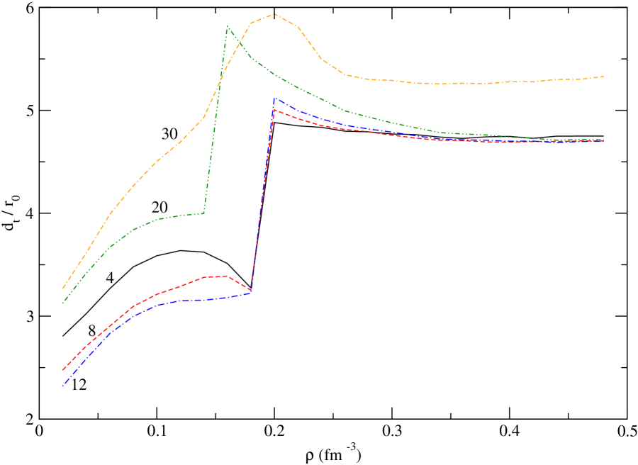
Figure 5: (Color online) The tensor correlation length in pure neutron matter. The numbers alongside the curves denote the temperature in MeV.

Generally particles are correlated over the longest range due to tensor interactions. In our calculations $d_{t}$ is one measure of this range. In Figs. 4 and 5 we show $d_{t}$ for symmetric nuclear matter and pure neutron matter, respectively, for various temperatures. In Fig. 4 we see a dramatic decrease in the value of $d_{t}/r_{0}$ below $\rho\sim 0.06$ fm^-3 for $T=4$ MeV in symmetric nuclear matter. This is a precursor to cluster formation. We will discuss this topic briefly in Section V.

One of the most interesting features of these plots is the sharp change in magnitude of $d_{t}/r_{0}$ at $\rho\sim 2\rho_{0}$ for symmetric nuclear matter and at $\rho\sim\rho_{0}$ for pure neutron matter. A similar feature was obtained in the zero temperature calculations of APR. In APR it was argued that this feature resulted from a first order phase transition due to neutral pion condensation Migdal (1978); Sawyer and Scalapino (1973). Their argument was based on the fact that the energy per particle as a function of density showed a kink indicating a first order phase transition, and that the isovector spin longitudinal reponse showed an enhancement and softening in the high density phase compared to the low density phase indicating enhanced pion exchange interactions between nucleons in the high density phase. Recently there has been some indication of experimental evidence supporting the enhancement of pionic modes in nuclei (see Ichimura et al. (2006) for a review).

The isovector spin longitudinal static structure function is defined as

$$S_{L}({\bf q})=\frac{1}{A}\left(\langle O_{L}^{2}\rangle_{T,\rho}-|\langle O_{L}\rangle_{T,\rho}|^{2}\right)\ ,$$ (48)

where

$$O_{L}({\bf q})=\sum_{i=1}^{A}\mbox{\boldmath$\sigma$}_{i}\cdot\hat{{\bf q}}\mbox{\boldmath$\tau$}_{i}\cdot\hat{{\bf t}}\mbox{e}^{i{\bf q}\cdot{\bf r}_{i}}\ .$$ (49)

Here ${\bf r}_{i}$ are the positions of the nucleons and $\hat{{\bf t}}$ is a unit vector in the isospin space. This quantity is also the sum of the isovector spin longitudinal dynamic response function $R_{L}({\bf q},\omega)$,

$$S_{L}(q)=\frac{1}{A}\int_{0}^{\infty}R_{L}({\bf q},\omega)\mbox{d}\omega$$ (50)

$$R_{L}({\bf q},\omega)=\sum_{I,J}p_{I}\left|\langle J|O_{L}({\bf q})|I\rangle\right|^{2}\delta(\omega_{J}-\omega_{I}-\omega)$$ (51)

where $I$ and $J$ are eigenstates of the Hamiltonian with eigenvalues $\omega_{I}$ and $\omega_{J}$, respectively, and $p_{I}$ is the probability of the state $I$ occurring in the thermal ensemble.

It is also possible to define a mean energy $\bar{E}_{L}(q)$ of the isovector spin longitudinal response by,

$$W_{L}(q)=\frac{1}{A}\int_{0}^{\infty}\omega R_{L}(q,\omega)\textrm{d}\omega$$ (52)

$$\bar{E}_{L}(q)=\frac{W_{L}(q)}{S_{L}(q)}$$ (53)

Both $S_{L}(q)$ and $W_{L}(q)$ and hence $\bar{E}_{L}(q)$ can be calculated from the two body densities $\rho^{p}_{2}(r)$.

In Fig. 6 we plot $S_{L}$ and $\bar{E}_{L}$ in symmetric nuclear matter at $T=4$, $10$ and $16$ MeV for various densities. For all three temperatures we see a big enhancement of $S_{L}$ at $q\sim 1.3$ fm^-1 due to stronger spin-isospin correlations at higher densities. However, for $T=4$ MeV the enhancement develops quite suddenly at $\rho=2\rho_{0}$ while at $T=10$ MeV and $16$ MeV there is a smoother evolution of the enhancement as the density is increased. Similarly the mean energy $\bar{E}_{L}$ develops a dip at $q\sim 1.3$ fm^-1 for all three temperatures, but quite sharply at $T=4$ MeV and relatively smoothly at $10$ and $16$ MeV as functions of density.

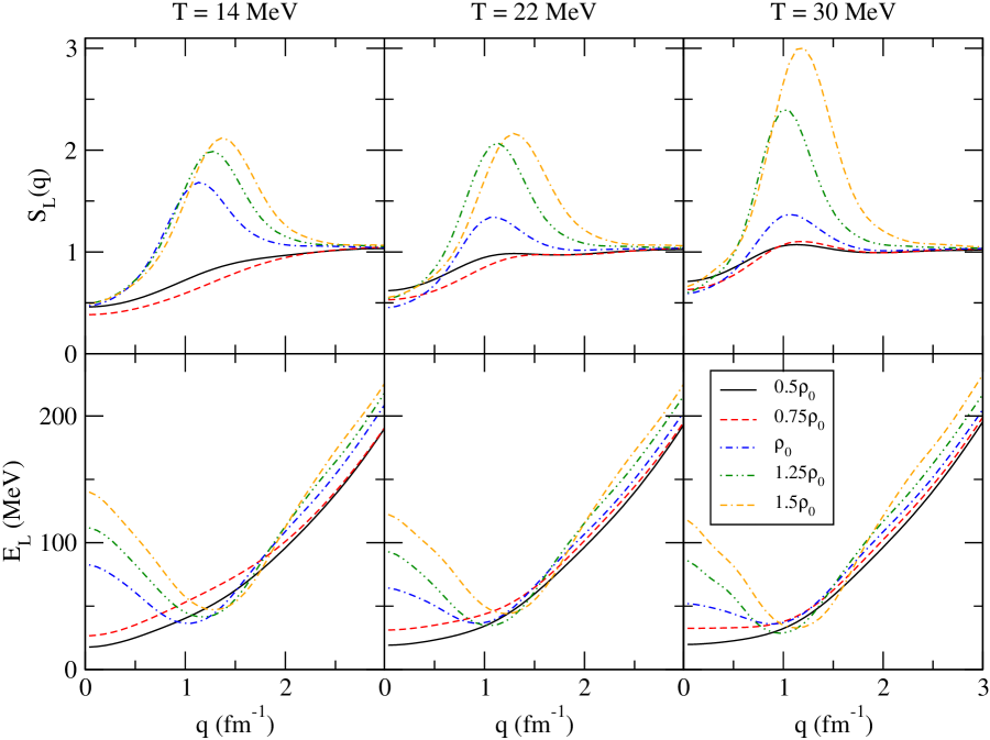
Figure 7: (Color online) The isovector spin longitudinal static structure function and mean energy in pure neutron matter.

The same quantities for pure neutron matter at $T=14$, $22$ and $30$ MeV are plotted in Fig. 7. Again, we see a large enhancement in the value $S_{L}$ for $\rho\geq\rho_{0}$ at $q\sim 1.3$ fm^-1 at all three temperatures. However the enhancement develops suddenly in the case of $T=14$ MeV, and relatively smoothly for $T=22$ and $30$ MeV. Also, the mean energy $\bar{E}_{L}$ shows a dip for densities $\rho\geq\rho_{0}$ at all temperatures, but this effect develops more smoothly at higher temperatures.

Our calculations thus show that the isovector spin longitudinal response for symmetric nuclear matter is enhanced and softened at densities $\rho\gtrsim 2\rho_{0}$ at finite temperatures. But whereas for $T<10$ MeV this enhancement and softening develops quite suddenly, there is a smoother evolution for $T\geq 10$ MeV. For pure neutron matter there is enhancement and softening of the isovector spin longitudinal response at densities $\rho\gtrsim\rho_{0}$, but it develops quite suddenly for $T<22$ MeV and quite smoothly for $T\geq 22$ MeV.

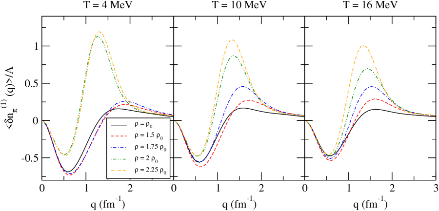
Figure 8: (Color online) The pion excess due to one pion exchange interactions in symmetric nuclear matter.

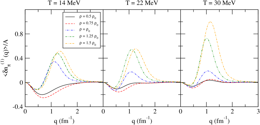
Figure 9: (Color online) The pion excess due to one pion exchange interactions in pure neutron matter.

The difference between the expectation values of the pion number operator in a system of $A$ interacting nucleons and in a system of $A$ isolated nucleons is called the pion excess. The part $\langle\delta_{\pi}^{(1)}(q)\rangle$ of the pion excess at a momentum ${\bf q}$, exclusively due to one pion exchange interactions, can be calculated from $S_{L}(q)$ Friman et al. (1983); Akmal and Pandharipande (1997). In Figs. 8 and 9 we show $\langle\delta_{\pi}^{(1)}(q)\rangle$ for symmetric nuclear matter and pure neutron matter. As with $S_{L}(q)$, $\langle\delta_{\pi}^{(1)}(q)\rangle$ shows an enhancement at higher densities. For symmetric nuclear matter this enhancement develops suddenly for $T<10$ MeV and smoothly for $T\gtrsim 10$ MeV. In pure neutron matter $T\approx 22$ MeV marks the temperature below which the enhancement is sudden and above which the enhancement is smooth.

The above observations along with the results for the equation of state (described in Section IV.3 below) leads us to conclude that the first order phase transition due to neutral pion condensation has a critical temperature of $T_{c}\approx 10$ MeV for symmetric nuclear matter and $T_{c}\approx 22$ MeV for pure neutron matter. Above the critical temperature the enhancement in the spin-isospin correlations still persists at higher densities, but now there is a smooth crossover between the low density phase and the high density phase.

IV.2 The Nucleon Effective mass

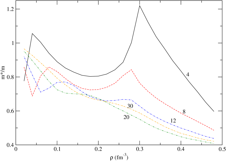
Figure 10: (Color online) The effective mass in symmetric nuclear matter. The numbers alongside the curves denote the temperature in MeV.

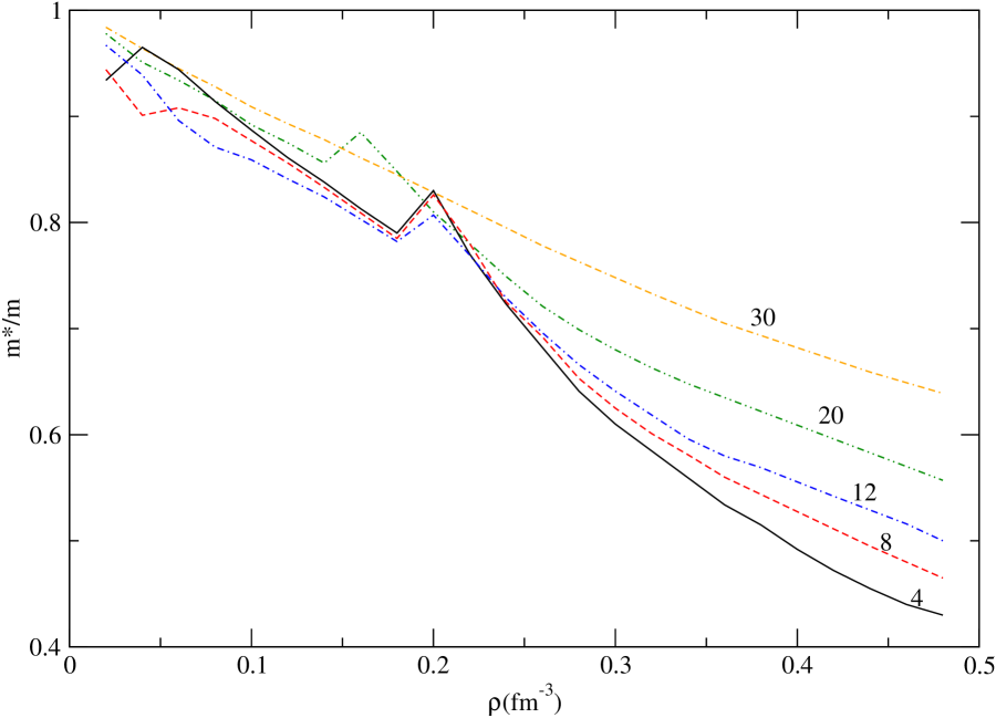
Figure 11: (Color online) The effective mass in pure neutron matter. The numbers alongside the curves denote the temperature in MeV.

The effective mass $m^{\star}$ is not only a variational parameter in our calculations, but also a quantity of considerable physical importance in determining the thermal properties of nuclear matter. Our results for $m^{\star}$ as a function of density in symmetric nuclear matter and pure neutron matter for various temperatures is shown in Figs. 10 and 11. We wish to point out that the variational minimization in pure neutron matter is not very sensitive to variations of $m^{\star}$, especially at low temperatures and the high density phase. In particular the uncertainty in our estimate of $m^{\star}$ for the high density phase in pure neutron matter for the three lowest temperatures reported ($4$, $8$ and $12$ MeV) is comparable to the total temperature dependence of $m^{\star}$ at these temperatures.

The curves of $m^{\star}$ vs $\rho$ show sharp changes at $\rho\sim 2\rho_{0}$ in symmetric nuclear matter and at $\rho\sim\rho_{0}$ in pure neutron matter. The origin of these changes is the enhancement of the spin-isospin correlations discussed earlier.

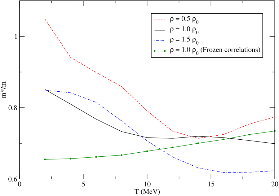
Figure 12: (Color online) The effective mass in symmetric nuclear matter at $\rho=0.5\rho_{0}$, $\rho_{0}$ and $1.5\rho_{0}$. Also plotted is the effective mass at $\rho=\rho_{0}$, obtained by using the frozen correlation method described in the text.

Our calculations also show an enhancement of $m^{\star}$ at low temperatures in symmetric nuclear matter and to a much lesser extent in pure neutron matter. This is clearer from Fig. 12 where $m^{\star}$ has been plotted as a function of temperature for $\rho=0.5\rho_{0}$, $\rho_{0}$ and $1.5\rho_{0}$ in symmetric nuclear matter. For example, for $\rho\sim\rho_{0}$, $m^{\star}$ at $T=2$ MeV is $0.85m$ and at $T=4$ MeV is $0.81m$ while at $T=20$ MeV it is $0.69m$ which is very close to the value $0.7m$ obtained from optical potential models of nucleon-nucleus scattering Bohr and Mottelson (1969); Jeukenne et al. (1976).

It is important to realize that the effective mass, defined as

$$m^{\star}(k)=k\frac{\mbox{d}k}{\mbox{d}\epsilon(k)}\ ,$$ (54)

can in general depend on the momentum $k$. The momentum independent effective mass $m^{\star}(\rho,T)$ that is used in the variational calculations is an weighted average of this momentum dependent $m^{\star}(k)$. It is difficult to establish the actual weighting given to each single particle state. However it is not difficult to convince oneself that at any given temperature and density the maximum contribution comes from states with single particle energies $\epsilon(k)$ such that

$$\left|\epsilon(k)-\epsilon(k_{F})\right|\lesssim\pi T$$ (55)

where $k_{F}$ is the Fermi momentum.

At very low temperatures only those single particle states which are very close to the Fermi surface can contribute. Theoretical calculations and experimental evidence suggests that the (momentum dependent) $m^{\star}(k)$ in symmetric nuclear matter has a big enhancement at and near the Fermi surface Jeukenne et al. (1976); Blaizot and Friman (1981); Krotscheck et al. (1981); Fantoni et al. (1983); Bohigas et al. (1979). In our calculations enhancement in $m^{\star}$ at low temperatures is probably due to this effect.

In FP no such enhancement was seen. For comparison, in Fig. 12 we have also plotted the $m^{\star}$ at $\rho=\rho_{0}$ obtained by simply minimizing $F_{v}$ and using correlation operator from the $T=0$ calculations, i.e. the frozen correlation method. This method is closest to the one used in FP albeit with different nucleon-nucleon interaction and three nucleon interaction. And indeed, we do not see any significant variation of $m^{\star}$ with temperature. In fact, the values of $m^{\star}/m$ so obtained are $0.66$, $0.68$, $0.71$, $0.73$ at $T=5$, $10$, $15$ and $20$ MeV, respectively. These are very close to the corresponding values $0.65$, $0.67$, $0.70$ and $0.73$ obtained by FP where the Urbana $v14$ model of the nucleon-nucleon interaction was used along with a density dependent term to simulate the effects of the three body forces.

It appears that we are able to capture some of the subtle correlations which influence the low energy quasiparticle excitations better because of the improvements introduced in our calculations. These improvements include the fact that in the variational search all the parameters were varied and the pair correlation functions were calculated at all temperatures, and the fact that we insist on satisfying the laws of conservation of mass and charge at the level of a few percents. However, this is simply one possibility since in general the free energy is not very sensitive to the variations in the effective mass and it is difficult to delineate the effect that each individual component in our method has on the effective mass. This topic deserves further investigation, and we hope to address it in more detail in future work Mukherjee .

IV.3 The Equation of State

As we discussed earlier the variational minimization for the optimal parameters $d_{t}$, $d_{c}$, $\alpha$ and $m^{\star}$ is carried out with $v_{18}+V_{\mbox{\tiny{UIX}}}$ only. Following APR some additional corrections were added to the energy.

1. The relativistic boost corrections $\delta v_{b}+(V^{\star}_{\mbox{\tiny{UIX}}}-V_{\mbox{\tiny{UIX}}})$ which were discussed earlier.

2. An estimate for the second order perturbative corrections $\Delta E_{2}$ is given by $\delta E_{2B}$ the difference between the two body cluster energy obtained by minimizing the contributions in each partial wave and the two body cluster energy obtained from the ${\cal F}_{ij}$ defined above.

3. An additional ad-hoc correction term $-\gamma_{2}\rho^{2}\mbox{e}^{-\gamma_{3}\rho}$, with $\gamma_{2}=1996$ MeV fm⁶ and $\gamma_{3}=15.24$ fm³ is added to the symmetric nuclear matter energy to get the correct saturation energy at zero temperature. These values are slightly different from those in APR ($\gamma_{2}=2822$ MeV fm⁶ and $\gamma_{3}=18.34$ fm³) because our variational energies and variational parameters at zero temperature are slightly different from those in APR owing to the improvements in the method described earlier.

Of the above only the relativistic boost corrections have a temperature dependence. The temperature dependence of the perturbative corrections was found to be negligible and was neglected. Thus our best estimate for the free energy is given by

$$F_{\mbox{\tiny{tot}}} = E_{v}-TS_{v}+E_{c}$$ (56)

$$= F_{v}+E_{c}$$ (57)

where $E_{c}$ is the sum of the correction terms mentioned above.

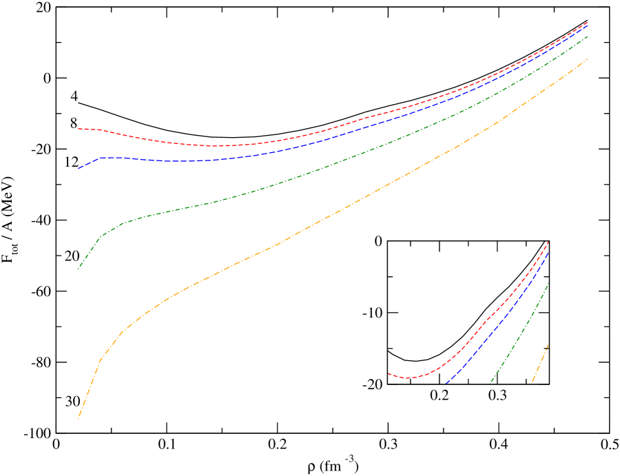
Figure 13: (Color online) The free energy in symmetric nuclear matter. The numbers alongside the curves denote the temperature in MeV. The inset shows in more detail the region of transition from the low density phase to the high density phase.

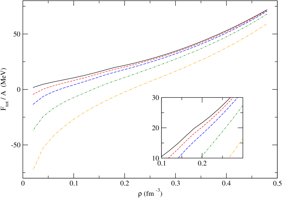
Figure 14: (Color online) The free energy in pure neutron matter. The numbers alongside the curves denote the temperature in MeV. The inset shows in more detail the region of transition from the low density phase to the high density phase.

The free energy $F_{\mbox{\tiny{tot}}}$ calculated using the method outlined in the last section is shown in Figs. 13 and 14 for symmetric nuclear matter and pure neutron matter, respectively, for temperatures $T=4-30$ MeV. The most striking feature in these figures is the sharp change in the slope of the free energy at low temperatures for both symmetric nuclear matter ($T<12$ MeV, $\rho\sim 0.30$ fm^-3) and pure neutron matter ($T<24$ MeV and $\rho\sim 0.18$ fm^-3) (see inset in Figs. 13 and 14).

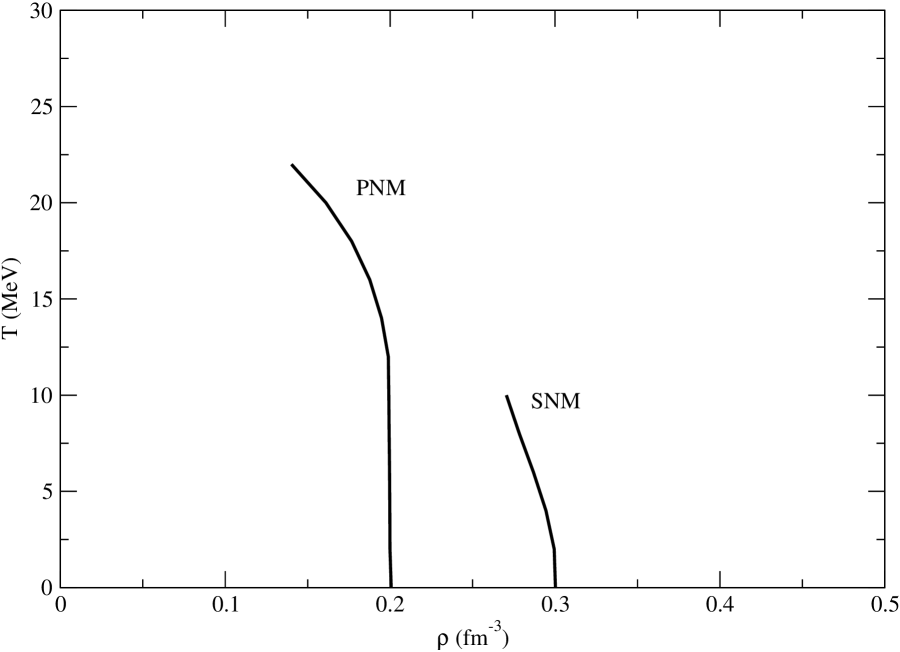
Figure 15: The transition density for neutral pion condensation for symmetric nuclear matter and pure neutron matter in the variational calculations.

During the variational search the global minimum of the free energy as a function of the variational parameters jumps from one local minimum to another. In Fig. 15 we show the density at which this transition from the low density phase to high density phase occurs in our calculations. This results in a first order phase transition. In light of our discussion in Section IV.1, we identify this phase transition with the phenomenon of the neutral pion condensation. As we mentioned in the earlier the critical temperature for this transition is $T_{c}\approx 10$ MeV for symmetric nuclear matter and $T_{c}\approx 22$ MeV for pure neutron matter.

At subsaturation densities and low temperatures symmetric nuclear matter undergoes another first order phase transition, the liquid-gas transition. In our calculations the critical temperature for the liquid-gas phase transition is $T_{c}\approx 21$ MeV and the critical density is about $\rho_{c}\sim 0.3\rho_{0}$. If the calculations are done using the variational free energy $F_{v}$ only, then the critical temperature for the liquid gas phase transition comes out to be about $16$ MeV. In the calculation due to FP the critical temperature is about $17.5$ MeV.

The pressure can be calculated from,

$$P(\rho,T)=\rho^{2}\left.\frac{\partial F/A}{\partial\rho}\right|_{T}\ .$$ (58)

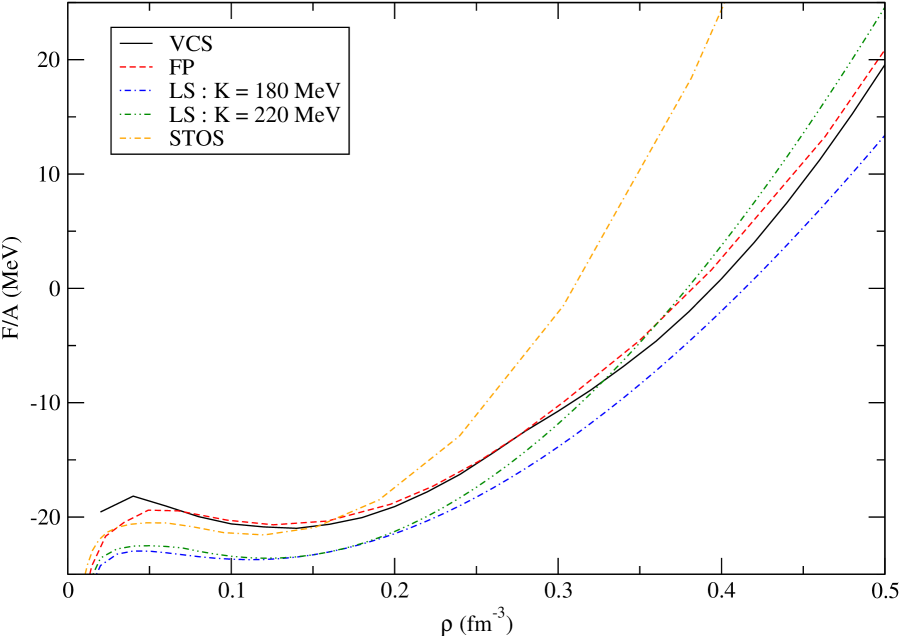
Figure 16: (Color online) A comparison of the free energy obtained using various methods at $T=10$ MeV. For an explanation of the various curves see the text.

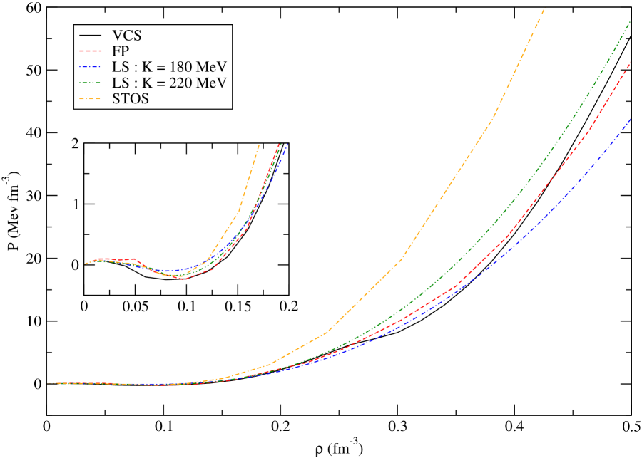
Figure 17: (Color online) A comparison of the pressure obtained using various methods at $T=10$ MeV. The inset shows the low density region in more detail. For an explanation of the various curves see the text.

Our estimates for the free energy $F(\rho,T)$ ($F_{\mbox{\tiny{tot}}}$ of Eq. (57)) and the pressure $P(\rho,T)$ of symmetric nuclear matter at $T=10$ MeV from the variational chain summation calculations have been plotted in Figs. 16 and 17 along with the same from some of the other popular equations of state viz. the equation of state due to FP, the Lattimer-Swesty (LS) liquid droplet model calculations with incompressibility $K=180$ and $220$ MeV Lattimer and Swesty (1991) and the equation of state due to Shen et al. (STOS) Shen et al. (1998a, b) which is based on relativistic mean field theory. The inset shows the pressure in the low density region in greater detail. We have kept the thermodynamically unstable region in the $P$ vs $\rho$ curve to facilitate comparison with the other equations of state. Due to the enhanced spin-isospin correlations our equation of state is relatively soft at $\rho\sim 2\rho_{0}$ fm^-3 but hardens at higher densities.

Various astrophysical phenomena depend sensitively on the symmetry energy $E_{\mbox{\tiny{sym}}}$ Lattimer and Prakash (2000) and the symmetry free energy $F_{\mbox{\tiny{sym}}}$ Xu et al. (2007) which are defined as

$$E_{\mbox{\tiny{sym}}} = \frac{1}{2}\left.\frac{\mbox{d}^{2}E}{\mbox{d}\delta^{2}}\right|_{\delta=0}$$ (59)

$$F_{\mbox{\tiny{sym}}} = \frac{1}{2}\left.\frac{\mbox{d}^{2}F}{\mbox{d}\delta^{2}}\right|_{\delta=0}\ .$$ (60)

Here $\delta$ is the asymmetry parameter given by

$$\delta=\frac{\rho_{n}-\rho_{p}}{\rho},$$ (61)

where $\rho_{n}$ is the neutron density and $\rho_{p}$ is the proton density. To the leading order in $\delta$, $E_{\mbox{\tiny{sym}}}$ is given by the difference between the energy in pure neutron matter $E_{\mbox{\tiny{PNM}}}$ and the energy in symmetric nuclear matter $E_{\mbox{\tiny{SNM}}}$. Similarly $F_{\mbox{\tiny{sym}}}$ is given by the difference between the free energy in pure neutron matter $F_{\mbox{\tiny{PNM}}}$ and symmetric nuclear matter $F_{\mbox{\tiny{SNM}}}$.

$$E_{\mbox{\tiny{sym}}} = E_{\mbox{\tiny{PNM}}}-E_{\mbox{\tiny{SNM}}}+{\cal O}(\delta^{2})$$ (62)

$$F_{\mbox{\tiny{sym}}} = F_{\mbox{\tiny{PNM}}}-F_{\mbox{\tiny{SNM}}}+{\cal O}(\delta^{2})\ .$$ (63)

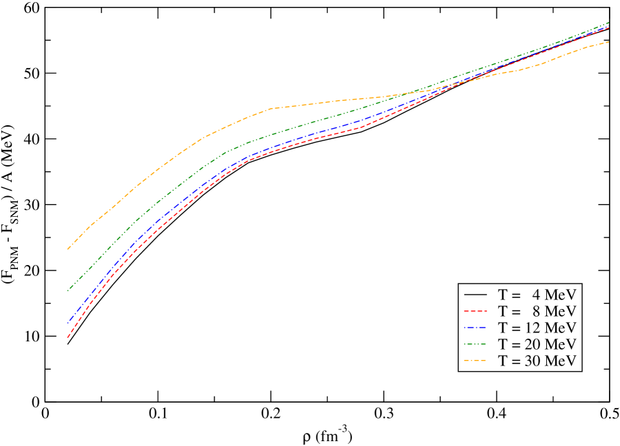
Figure 19: (Color online) A comparison of $F_{\mbox{\tiny{PNM}}}-F_{\mbox{\tiny{SNM}}}$ at various temperatures

In Figs. 17 and 19 we show $E_{\mbox{\tiny{PNM}}}-E_{\mbox{\tiny{SNM}}}$ and $F_{\mbox{\tiny{PNM}}}-F_{\mbox{\tiny{SNM}}}$ as functions of density at various temperatures.

V Discussion

In this section we will discuss the limitations of our calculations. First, let us consider the validity of the quasiparticle picture at finite temperature. This assumption is motivated by Landau’s theory of Fermi liquids. However Landau’s theory in its original formulation applies only to systems at zero or very low temperatures. It is justified on the basis of the fact that low lying quasiparticle excitations (as defined by the poles in the single particle propagator) are long lived at low temperatures Baym and Pethick (1978); Abrikosov and Khalatnikov (1959). At higher temperatures this is not true and one cannot associate well defined quasiparticle excitations to the system.

It is, however, important to recognize that there are two separate issues involved here. On the one hand, we have the thermodynamical statement that the free energy of the system can be written as a functional of quasiparticle occupation numbers and that in particular the entropy is given by Eq. (18). On the other hand, we have one particular microscopic justification of the previous statement in terms of the long lived nature of the quasiparticle excitations. It has been shown in the past that although the latter is true only for very low temperatures, the former, under very general conditions, is true for arbitrary temperatures Balian and de Dominicis (1971); de Dominicis (1960); Luttinger (1968); Pethick and Carneiro (1973); Carneiro and Pethick (1975). With this in mind we think that our final estimate for the free energy is more reliable than the individual components that entered the calculations, e.g. the assumption of an one-to-one mapping between the states of a non interacting system and an interacting one is not exactly true at for the states relevant at any finite temperature. However, even with this caveat in mind, we believe that our predictions about the microscopic structure of the system are useful in accounting for at least the gross features if not the details in the many body system.

Our description of the high density phase is clearly incomplete. Our wave function does not include any true long range order. It has been shown from very general arguments by Landau and Peierls that long range order where the order parameter varies only in one dimension is unstable at finite temperatures Baym et al. (1982). However, condensates that vary in two or three dimensions can exist at any temperature. If the high density phase is indeed a state with broken symmetry then it is possible that the first order transition changes into a second order transition beyond critical temperature (instead of a smooth crossover from the low density phase to the high density phase seen in our calculations). From our calculations we cannot make any prediction about this possibility.

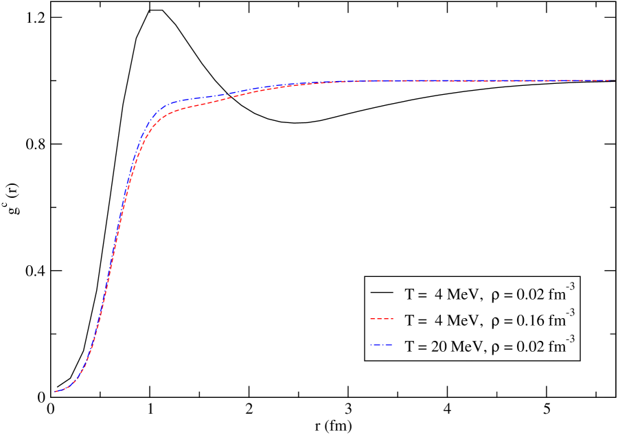
Figure 20: (Color online) The normalized pair distribution function at $T=4$ MeV and $\rho=0.02$ fm^-3 shows the effects of deuteron clustering. The same function has been plotted for $T=20$ and $\rho=0.02$ fm^-3 and $T=4$ MeV, and $\rho=0.16$ fm^-3 for comparison.

In the low density and low temperature region for symmetric nuclear matter the uniform fluid is no longer the optimal configuration and few body clusters are expected to emerge (see e.g. Ropke (2001)). We see the precursor to deuteron clustering in our calculations, e.g. in Fig. 20 we see that the pair distribution function for symmetric nuclear matter at $\rho=0.02$ fm^-3 and $T=2$ MeV shows a pronounced bump at $r\sim 1$ fm. Genuine clustering of three or more particles, however, is not possible in our variational chain summation calculations because our wave functions are too simple to describe such phenomena.

Another phenomenon which occurs at very low densities and temperatures in nuclear matter is superfluidity due to the formation of Cooper pairs Dean and Hjorth-Jensen (2003); Sedrakian and Clark (2006). Pairing, especially in very low density pure neutron matter and neutron star matter, has been the subject of extensive research in the recent past Lombardo and Schulze (2001) (and references therein). The wave functions that we have used do not include the effects of pairing in the long range part. However we would like to point out that it is possible to develop a variational theory based on correlated basis states for superfluid systems at zero temperatures Fantoni (1981); Fabrocini et al. (2008). It is quite possible that this theory can be extended to finite temperatures in a manner very similar to the one used here for normal systems.

At very high temperatures ($T\gtrsim 50$ MeV for symmetric nuclear matter) thermal excitations of the pionic degrees of freedom, the ‘thermal pions’ Kolehmainen and Baym (1982) become important and should be explicitly included in the equation of state Friedman et al. (1981) . Our present calculations do not have any explicit non-nucleonic degrees of freedom, thus they cannot be extended to very high temperatures without the explicit inclusion of the thermal pions. The calculation of the pionic spectrum in nuclear matter is a challenging task. However, as the first step, the simplified quasiparticle treatment of the pions along with the full variational chain summation calculation for the nucleons as done in Ref. Friedman et al. (1981) might prove useful.

Finally, we would briefly discuss the case of arbitrary proton fraction. Pure variational chain summation can only be used to calculate the equation of state of symmetric nuclear matter and pure neutron matter, and not for asymmetric nuclear matter. This problem can be circumvented by using the so called quadratic approximation, where one assumes that the interaction energy at an arbitrary asymmetry $\delta$ has a purely quadratic dependence on $\delta$. Using this fact the energy for any $\delta$ can be found from the results at $\delta=0$ (symmetric nuclear matter ) and $\delta=1$ (pure neutron matter) Akmal et al. (1998); Pandharipande and Ravenhall (1989).

It has been shown in Ref. Lagaris and Pandharipande (1981) that within the scheme of variational calculations (although with a lower order approximation for the non-central correlations as compared to the variational chain summation method) the quadratic approximation is quite accurate, at least up to the leading order terms in the interaction energy. This calculation was done for the zero temperature low density phase, with the Urbana $v_{14}$ model for nucleon-nucleon interaction and a density dependent model for three nucleon interaction. Thus far, the calculation has not been repeated for finite temperatures, the high density phase or for the modern sets of nucleon-nucleon interaction and three nucleon interaction. It is, however, plausible that the result is true for the aforementioned conditions as well.

VI Conclusion

The calculation of the properties of nuclear matter in supernovae, neutron stars and heavy ion collisions starting from the properties of nucleons in vacuum and light nuclei is an outstanding problem in nuclear many body theory. In a preceding paper (I) we showed that when the variational theory is extended to finite temperatures, the free energy and the single particle energies do not have any corrections due to the non-orthogonality of the correlated basis states used in these variational theories. In this paper we showed how this formalism can be used for practical calculations in hot dense nucleon matter.

We calculated the equation of state of symmetric nuclear matter and pure neutron matter and discussed the fate of the neutral pion condensation at finite temperature. The first order phase transition was seen to have a critical temperature of about $10$ MeV for symmetric nuclear matter and about $22$ MeV for pure neutron matter. However, the the enhancement of the spin-isospin correlations and as a result the softening of the equation of state, near $\rho\sim 2\rho_{0}$ for symmetric nuclear matter and near $\rho\sim\rho_{0}$ for pure neutron matter, persists even beyond the critical temperature. We also discussed the behavior of the nucleon effective mass and saw an enhancement at lower temperatures. We proposed one possible explanation for this effect.

The pair correlation functions ${\cal F}_{ij}$ generated during our variational minimizations can be used to calculate the equation of state of asymmetric nuclear matter within the quadratic approximation Pandharipande and Ravenhall (1989), the single particle energies in dense nuclear matter Friedman and Pandharipande (1981b); Wiringa (1988), effective interactions Cowell and Pandharipande (2003, 2006) and transport properties Benhar and Valli (2007). Some of these topics will be explored in our future work Mukherjee .

Figure 1: (Color online) The pair correlation function in the central channel of symmetric nuclear matter various densities and temperatures.

Figure 2: (Color online) The pair correlation function in the tensor-isospin channel of symmetric nuclear matter various densities and temperatures.

Figure 3: (Color online) The two body densities in symmetric nuclear matter at saturation density and different temperatures.

Figure 4: (Color online) The tensor correlation length in symmetric nuclear matter. The numbers alongside the curves denote the temperature in MeV.

Figure 6: (Color online) The isovector spin longitudinal static structure function and mean energy in symmetric nuclear matter.

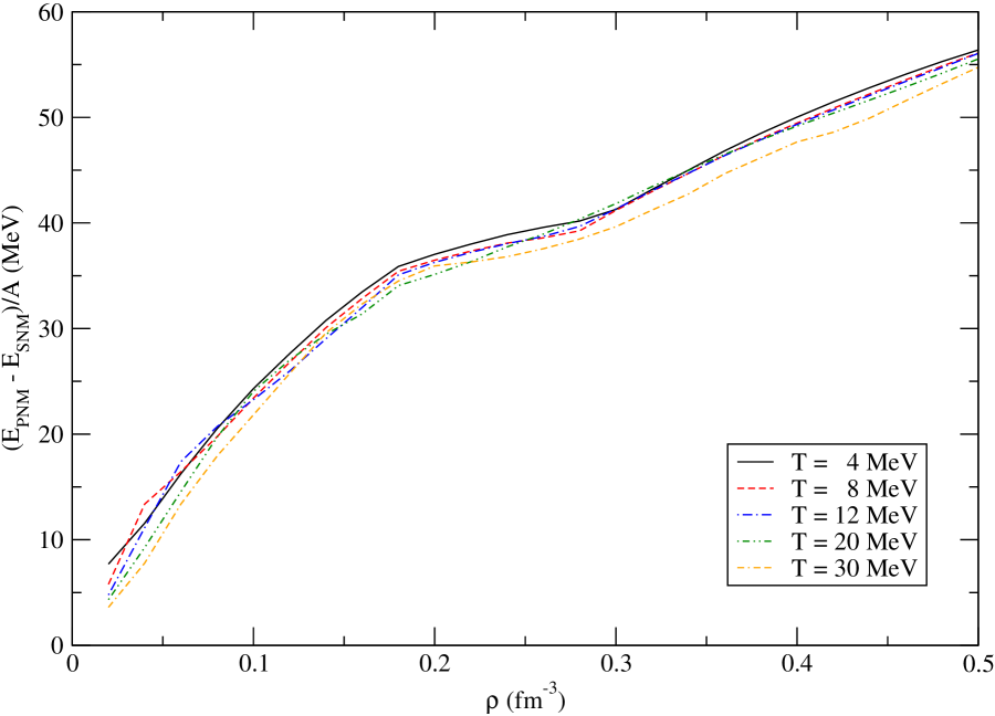
Figure 18: (Color online) A comparison of $E_{\mbox{\tiny{PNM}}}-E_{\mbox{\tiny{SNM}}}$ at various temperatures

References

- Lattimer and Prakash (2000) J. M. Lattimer and M. Prakash, Phys. Rep. 333, 121 (2000).
- Janka et al. (2007) H.-T. Janka, K. Langanke, A. Marek, G. Martínez-Pinedo, and B. Müller, Phys. Rep. 442, 38 (2007).
- Prakash et al. (1997) M. Prakash, I. Bombaci, M. Prakash, P. J. Ellis, J. M. Lattimer, and R. Knorren, Phys. Rep. 280, 1 (1997).
- Pons et al. (1999) J. A. Pons, S. Reddy, M. Prakash, J. M. Lattimer, and J. A. Miralles, ApJ 513, 780 (1999).
- Oechslin and Janka (2007) R. Oechslin and H.-T. Janka, Physical Review Letters 99, 121102 (2007).
- Li et al. (2008) B.-A. Li, L.-W. Chen, and C. M. Ko, Phys. Rep. 464, 113 (2008).
- Heiselberg and Pandharipande (2000) H. Heiselberg and V. Pandharipande, Ann. Rev. Nucl. Part. Sci. 50, 481 (2000).
- Baldo et al. (1995) M. Baldo, G. Giansiracusa, U. Lombardo, I. Bombaci, and L. S. Ferreira, Nucl. Phys. A583, 599 (1995).
- Lattimer and Swesty (1991) J. M. Lattimer and F. D. Swesty, Nucl. Phys. A535, 331 (1991).
- Shen et al. (1998a) H. Shen, H. Toki, K. Oyamatsu, and K. Sumiyoshi, Nucl. Phys. A637, 435 (1998a).
- Shen et al. (1998b) H. Shen, H. Toki, K. Oyamatsu, and K. Sumiyoshi, Prog. Theo. Phys. 100, 1013 (1998b).
- Friedman and Pandharipande (1981a) B. Friedman and V. R. Pandharipande, Nucl. Phys. A361, 502 (1981a).
- Baldo and Ferreira (1999) M. Baldo and L. S. Ferreira, Phys. Rev. C 59, 682 (1999).
- Lejeune et al. (1986) A. Lejeune, P. Grange, M. Martzolff, and J. Cugnon, Nucl. Phys. A453, 189 (1986).
- Zuo et al. (2004) W. Zuo, Z. H. Li, A. Li, and G. C. Lu, Phys. Rev. C 69, 064001 (2004).
- Rios et al. (2006) A. Rios, A. Polls, A. Ramos, and H. Müther, Phys. Rev. C 74, 054317 (2006).
- ter Haar and Malfliet (1986) B. ter Haar and R. Malfliet, Phys. Rev. Lett. 56, 1237 (1986).
- Huber et al. (1998) H. Huber, F. Weber, and M. K. Weigel, Phys. Rev. C 57, 3484 (1998).
- Tolos et al. (2008) L. Tolos, B. Friman, and A. Schwenk, Nucl. Phys. A806, 105 (2008).
- Kanzawa et al. (2007) H. Kanzawa, K. Oyamatsu, K. Sumiyoshi, and M. Takano, Nucl. Phys. A791, 232 (2007).
- Jastrow (1955) R. Jastrow, Phys. Rev. 98, 1479 (1955).
- Clark (1979) J. W. Clark, Prog. Part. Nucl. Phys. 2, 89 (1979).
- Pandharipande and Wiringa (1979) V. R. Pandharipande and R. B. Wiringa, Rev. Mod. Phys. 51, 821 (1979).
- Akmal and Pandharipande (1997) A. Akmal and V. R. Pandharipande, Phys. Rev. C 56, 2261 (1997).
- Wiringa et al. (1988) R. B. Wiringa, V. Fiks, and A. Fabrocini, Phys. Rev. C 38, 1010 (1988).
- Akmal et al. (1998) A. Akmal, V. R. Pandharipande, and D. G. Ravenhall, Phys. Rev. C 58, 1804 (1998).
- Morales et al. (2002) J. Morales, V. R. Pandharipande, and D. G. Ravenhall, Phys. Rev. C 66, 054308 (2002).
- Danielewicz et al. (2002) P. Danielewicz, R. Lacey, and W. G. Lynch, Science 298, 1592 (2002).
- Carlson et al. (2003) J. Carlson, J. Morales, V. R. Pandharipande, and D. G. Ravenhall, Phys. Rev. C 68, 025802 (2003).
- Schmidt and Pandharipande (1979) K. E. Schmidt and V. R. Pandharipande, Phys. Lett. B 87, 11 (1979).
- Fantoni and Pandharipande (1988) S. Fantoni and V. R. Pandharipande, Phys. Rev. C 37, 1697 (1988).
- Mukherjee and Pandharipande (2007) A. Mukherjee and V. R. Pandharipande, Phys. Rev. C 75, 035802 (2007).
- Wiringa et al. (1995) R. B. Wiringa, V. G. J. Stoks, and R. Schiavilla, Phys. Rev. C 51, 38 (1995).
- Carlson et al. (1983) J. Carlson, V. R. Pandharipande, and R. B. Wiringa, Nucl. Phys. A401, 59 (1983).
- Pudliner et al. (1995) B. S. Pudliner, V. R. Pandharipande, J. Carlson, and R. B. Wiringa, Phys. Rev. Lett. 74, 4396 (1995).
- Forest et al. (1995) J. L. Forest, V. R. Pandharipande, and J. L. Friar, Phys. Rev. C 52, 568 (1995).
- Machleidt et al. (1996) R. Machleidt, F. Sammarruca, and Y. Song, Phys. Rev. C 53, R1483 (1996).
- Machleidt (2001) R. Machleidt, Phys. Rev. C 63, 024001 (2001).
- Stoks et al. (1994) V. G. J. Stoks, R. A. M. Klomp, C. P. F. Terheggen, and J. J. de Swart, Phys. Rev. C 49, 2950 (1994).
- Carlson et al. (1993) J. Carlson, V. R. Pandharipande, and R. Schiavilla, Phys. Rev. C 47, 484 (1993).
- Feynman (1972) R. P. Feynman, Statistical Mechanics (Benjamin, 1972).
- Pandharipande and Ravenhall (1989) V. R. Pandharipande and D. G. Ravenhall, in NATO ASIB Proc. 205: Nuclear Matter and Heavy Ion Collisions, edited by M. Soyeur, H. Flocard, B. Tamain, and M. Porneuf (1989), p. 103.
- Nelder and Mead (1965) J. A. Nelder and R. Mead, Comput. J. 7, 308 (1965).
- (44) J. Morales, private communication.
- Migdal (1978) A. B. Migdal, Rev. Mod. Phys. 50, 107 (1978).
- Sawyer and Scalapino (1973) R. F. Sawyer and D. J. Scalapino, Phys. Rev. D 7, 953 (1973).
- Ichimura et al. (2006) M. Ichimura, H. Sakai, and T. Wakasa, Prog. Part. Nucl. Phys. 56, 446 (2006).
- Friman et al. (1983) B. L. Friman, V. R. Pandharipande, and R. B. Wiringa, Phys. Rev. Lett. 51, 763 (1983).
- Bohr and Mottelson (1969) A. Bohr and B. Mottelson, Nuclear Structure vol. 1 (Benjamin, New York, 1969).
- Jeukenne et al. (1976) J. P. Jeukenne, A. Lejeune, and C. Mahaux, Phys. Rep. 25, 83 (1976).
- Blaizot and Friman (1981) J. P. Blaizot and B. L. Friman, Nucl. Phys. A372, 69 (1981).
- Krotscheck et al. (1981) E. Krotscheck, R. A. Smith, and A. D. Jackson, Phys. Lett. B 104, 421 (1981).
- Fantoni et al. (1983) S. Fantoni, B. L. Friman, and V. R. Pandharipande, Nucl. Phys. A399, 51 (1983).
- Bohigas et al. (1979) O. Bohigas, A. M. Lane, and J. Martorell, Phys. Rep. 51, 267 (1979).
- (55) A. Mukherjee, in preparation.
- Xu et al. (2007) J. Xu, L.-W. Chen, B.-A. Li, and H.-R. Ma, Phys. Rev. C 75, 014607 (2007).
- Baym and Pethick (1978) G. A. Baym and C. Pethick, Landau Fermi-liquid theory : concepts and applications (Wiley, New York, 1978).
- Abrikosov and Khalatnikov (1959) A. A. Abrikosov and I. M. Khalatnikov, Rep. Prog. Phys. 22, 329 (1959).
- Balian and de Dominicis (1971) R. Balian and C. de Dominicis, Ann. Phys. 62, 229 (1971).
- de Dominicis (1960) C. de Dominicis, Physica 26, 94 (1960).
- Luttinger (1968) J. M. Luttinger, Phys. Rev. 174, 263 (1968).
- Pethick and Carneiro (1973) C. J. Pethick and G. M. Carneiro, Phys. Rev. A 7, 304 (1973).
- Carneiro and Pethick (1975) G. M. Carneiro and C. J. Pethick, Phys. Rev. B 11, 1106 (1975).
- Baym et al. (1982) G. Baym, B. L. Friman, and G. Grinstein, Nucl. Phys. B210, 193 (1982).
- Ropke (2001) G. Ropke, in Condensed Matter Theories (2001), vol. 16, pp. 469–480.
- Dean and Hjorth-Jensen (2003) D. J. Dean and M. Hjorth-Jensen, Rev. Mod. Phys. 75, 607 (2003).
- Sedrakian and Clark (2006) A. Sedrakian and J. W. Clark, Nuclear Superconductivity in Compact Stars: BCS Theory and Beyond (Pairing in Fermionic Systems: Basic Concepts and Modern Applications, 2006), p. 135.
- Lombardo and Schulze (2001) U. Lombardo and H.-J. Schulze, in Physics of Neutron Star Interiors (2001), vol. 578 of Lecture Notes in Physics, Berlin Springer Verlag, p. 30.
- Fantoni (1981) S. Fantoni, Nucl. Phys. A363, 381 (1981).
- Fabrocini et al. (2008) A. Fabrocini, S. Fantoni, A. Y. Illarionov, and K. E. Schmidt, Nucl. Phys. A803, 137 (2008).
- Kolehmainen and Baym (1982) K. Kolehmainen and G. Baym, Nucl. Phys. A382, 528 (1982).
- Friedman et al. (1981) B. Friedman, V. R. Pandharipande, and Q. N. Usmani, Nucl. Phys. A372, 483 (1981).
- Lagaris and Pandharipande (1981) I. E. Lagaris and V. R. Pandharipande, Nucl. Phys. A369, 470 (1981).
- Friedman and Pandharipande (1981b) B. Friedman and V. R. Pandharipande, Phys. Lett. B 100, 205 (1981b).
- Wiringa (1988) R. B. Wiringa, Phys. Rev. C 38, 2967 (1988).
- Cowell and Pandharipande (2003) S. Cowell and V. R. Pandharipande, Phys. Rev. C 67, 035504 (2003).
- Cowell and Pandharipande (2006) S. Cowell and V. R. Pandharipande, Phys. Rev. C 73, 025801 (2006).
- Benhar and Valli (2007) O. Benhar and M. Valli, Phys. Rev. Lett. 99, 232501 (2007).