Bubbling route to strange nonchaotic attractor in a nonlinear series LCR circuit with a nonsinusoidal force

Abstract

We identify a novel route to the birth of a strange nonchaotic attractor (SNA) in a quasiperiodically forced electronic circuit with a nonsinusoidal (square wave) force as one of the quasiperiodic forces through numerical and experimental studies. We find that bubbles appear in the strands of the quasiperiodic attractor due to the instability induced by the additional square wave type force. The bubbles then enlarge and get increasingly wrinkled as a function of the control parameter. Finally, the bubbles get extremely wrinkled (while the remaining parts of the strands of the torus remain largely unaffected) resulting in the birth of the SNA which we term as the bubbling route to SNA. We characterize and confirm this birth from both experimental and numerical data by maximal Lyapunov exponents and their variance, Poincaré maps, Fourier amplitude spectra and spectral distribution function. We also strongly confirm the birth of SNA via the bubbling route by the distribution of the finite-time Lyapunov exponents.

I Introduction

Strange nonchaotic attractors (SNAs) are considered as typical structures of quasiperiodically forced nonlinear systems. They are geometrically strange (that is they are fractal in nature) just like the chaotic attractors, while all their Lyapunov exponents are either zero or negative which ensure that the underlying dynamics is nonchaotic. Further, due to their fractal nature, the SNAs are characterized by aperiodic oscillations. Following the pioneering work of Grebogi et al. Grebogi et al. (1984), SNAs have been extensively investigated theoretically in several dynamical systems  Romeiras and Ott (1987); Bondeson et al. (1985); Ding et al. (1989); Heagy and Ditto (1991); Yalcinkaya and Lai (1996); Kapitaniak and Wojewoda (1993); Venkatesan et al. (2000); Venkatesan and Lakshmanan (1997); Prasad et al. (1997); Pikovsky and Feudel (1995); Anishchensko et al. (1996); Nishikawa and Kaneko (1996); Venkatesan and Lakshmanan (2001); Hunt and Ott (2001); Heagy and Hammel (1994); Prasad et al. (1999); Zhou and Chen (1997); Kim and Lim (2004); Kapitaniak et al. (1997). The existence of SNAs has also been demonstrated experimentally Yang and Bilimgut (1997); Ditto et al. (1990); Venkatesan et al. (1999); Thamilmaran et al. (2006) in a few physically relevant situations. As a consequence, several routes (scenarios having distinct signatures) to SNAs have been reported theoretically. These include Heagy-Hammel route Heagy and Hammel (1994), gradual fractalization route Nishikawa and Kaneko (1996), various types of intermittency routes Venkatesan et al. (1999); Prasad et al. (1997); Hunt and Ott (2001); Kim and Lim (2004), blowout bifurcation route Yalcinkaya and Lai (1996), etc. As all these bifurcation scenarios (routes to SNAs) have been well established in the literature, we summarize the different scenarios for the formation of SNAs along with their distinct signatures/mechanisms in Table I. Reviews on SNAs can be found in Refs. Kapitaniak and Wojewoda (1993); Kapitaniak et al. (1997); Kapitaniak and Wojewoda (1993).

As mentioned above, while extensive numerical studies on the birth of SNAs via different routes are available in the literature  Romeiras and Ott (1987); Bondeson et al. (1985); Ding et al. (1989); Heagy and Ditto (1991); Yalcinkaya and Lai (1996); Kapitaniak and Wojewoda (1993); Venkatesan et al. (2000); Venkatesan and Lakshmanan (1997); Prasad et al. (1997); Pikovsky and Feudel (1995); Anishchensko et al. (1996); Nishikawa and Kaneko (1996); Venkatesan and Lakshmanan (2001); Hunt and Ott (2001); Heagy and Hammel (1994); Prasad et al. (1999); Zhou and Chen (1997); Kim and Lim (2004); Kapitaniak et al. (1997), only a few experimental realizations of them exist  Yang and Bilimgut (1997); Ditto et al. (1990); Venkatesan et al. (1999); Thamilmaran et al. (2006). In particular, these exotic attractors were confirmed by an experiment consisting of a quasiperiodically forced, buckled, magneto-elastic ribbon Ditto et al. (1990). SNAs were also realized in analog simulations of a multistable potential Zhou et al. (1992), and in a neon glow discharge experiment Ding et al. (1997). These attractors were also shown to be related to the Anderson localization phenomenon in the Schr$\ddot{\text{o}}$dinger equation with a quasiperiodic potential Ketoja and Satija (1997); Prasad et al. (1999). Very recently SNAs have also been observed in an excitable chemical system, namely a three electrode electrochemical cell Ruiz and Parmananda (2007). In this connection, from an experimental point of view, nonlinear electronic circuits with suitable quasiperiodic forces turn out to be especially useful dynamical systems for the identification and study of SNAs. For example, Type-I intermittency route to SNA was reported in a quasiperiodically forced Murali-Lakshmanan-Chua circuit Venkatesan et al. (1999). Recently, three prominent routes, namely Heagy-Hammel, fractalization and type-III intermittency routes to SNAs, have been identified and reported in a quasiperiodically forced negative conductance series LCR circuit with a diode Thamilmaran et al. (2006) both experimentally and numerically by some of the present authors.

In almost all the above studies, as a general rule, the driving forces are assumed to be sinusoidal in nature. Naturally the question arises as to what happens to the dynamics when one or both of the driving forces are nonsinusoidal but periodic. Can new routes to the birth of SNAs emerge in such a scenario? In order to answer these questions, we consider the quasiperiodically driven negative conductance series LCR circuit with a diode (which was investigated in  Thamilmaran et al. (2006)) and unravel the dynamics of the circuit with one of the forces taken as a square wave force (nonsinusoidal) for suitable parameter values. The main reason for choosing square wave as one of the driving forces is its bistable nature. Bistability is responsible for hysteresis in many physical and technical systems Thamilmaran et al. (2006, 2006, 2006, 2006). Further, the square wave has also been used for inducing chaos in certain dynamical systems Thamilmaran et al. (2006). For example a 10 MHz square wave optical message was injected into a ring laser to produce high-dimensional chaotic light Thamilmaran et al. (2006). Thus the study of the present circuit has considerable relevance in understanding SNA transitions.

Table 1: Routes and mechanisms for the formation of SNAs

Type of route	Mechanism
Heagy-Hammel Heagy and Hammel (1994)	Collision of period-doubled torus
	with its unstable parent
Gradual Fractilization Nishikawa and Kaneko (1996)	Increased wrinkling of torus
	without any interaction with
	nearby periodic orbits
Type-I intermittency Prasad et al. (1997)	Due to saddle-node bifurcation,
	a torus is replaced by SNA
Type-III intermittency Venkatesan et al. (1999)	Subharmonic instability
Crisis-induced intermittency	Doubling of destroyed torus
Venkatesan and Lakshmanan (2001)	involves a kind of sudden
	widening of the attractor
Homoclinic collision Prasad et al. (1999)	Homoclinic collisions of the
	quasiperiodic orbits
Blowout bifurcation Yalcinkaya and Lai (1996)	Due to changes in sign of the
	Lyapunov exponent $\Lambda_{T}$ transverse
	to the invariant subspace $S$
Quasiperiodic route Pikovsky and Feudel (1995); Venkatesan and Lakshmanan (1997)	Collision between a stable
	and unstable torus

In the present proposed circuit with a square wave force as one of the quasiperiodic forces in addition to a sinusoidal force, we have identified a new route for the formation of SNA which we term as the bubbling route to SNA. In this route bubbles appear in the strands of the torus as a function of the control parameter, then the sizes of the bubbles increase with the value of the control parameter and subsequently strands of the bubbles are increasingly wrinkled resulting in the birth of SNA (while the remaining parts of the strands of the torus outside the bubbles remain largely unaffected). The mechanism for this route is that the quasiperiodic orbit becomes increasingly unstable in its transverse direction as a function of the control parameter which is induced by the square wave type quasiperiodic force resulting in an increase in the size of the doubled strands (bubbles) in certain parts of the main strand and then the doubled strands become extremely wrinkled (without a complete doubling of the entire main strand) resulting in the SNA. In addition to this we have also observed four other prominent routes in the same circuit which include fractalization, fractalization followed by intermittency, intermittency and Heagy-Hammel routes, the details of which will be published elsewhere.

In order to confirm the existence of the bubbling route to SNA in the proposed circuit, we first present a detailed numerical analysis of the dynamical equations of the circuit in a rescaled form for suitable values of the parameters using various qualitative and quantitative measures to establish this route. These include Poincaré surface of section, Fourier spectrum, largest Lyapunov exponent and its variance, spectral distribution function and distribution of finite time Lyapunov exponents. A short account of these measures is given in Appendix A. Next, we confirm the results experimentally by the phase portraits of the quasiperiodic attractors and SNAs for the corresponding values of the circuit parameters, again with appropriate quantification measures, to establish the existence of torus and the birth of SNA through the bubbling route.

The paper is organized as follows. In Sec. II, we discuss the circuit realization of the quasiperiodically forced negative conductance series LCR circuit with diode using a sinusoidal and a nonsinusoidal (square wave) forcing as quasiperiodic forces. In Sec. III, we describe the phase diagram of the circuit where the regions corresponding to the different dynamical transitions to SNAs are delineated as a function of the control parameters, based on our numerical analysis. The birth of SNA via the bubbling route as confirmed in the numerical analysis is discussed in Sec. IV. Experimental confirmation of the bubbling route to SNA is presented in Sec. V. Finally, we summarize our results in Sec. VI. Appendix A contains a short summary on the identification and characterization of SNA and the associated routes.

II Circuit realization

In this section details about the proposed circuit are presented and the circuit equations are written in terms of the circuit variables. Then the circuit equations are transformed into dimensionless equations (normalized equations) using appropriate rescaled variables for a convenient numerical analysis.

II.1 Experimental realization: Circuit Equations

We consider the simple second-order nonlinear dissipative nonautonomous negative conductance series LCR circuit with a sinusoidal voltage generator, $f_{1}(t)$, introduced by us very recently Thamilmaran et al. (2005, 2006) along with a second nonsinusoidal force, $f_{2}(t)$, as shown in Fig. 1a.

Figure 1: (a) Circuit realization of a simple nonautonomous circuit. Here $D$ is the p-n junction diode and $g_{N}$ is negative conductance. The external emfs are $f_{1}(t)=E_{f1}\sin(\omega_{f1}t)$ and $f_{2}(t)=E_{f2}sgn(\sin(\omega_{f2}t))$. The values of the circuit elements are fixed as $L=50.3~{}mH$, $C=10.35~{}nF$, $R=1900ohms$, $E_{f2}=400mV$ and $\omega_{f2}=17033Hz$. The forcing amplitude $E_{f1}$ and its frequency $\omega_{f1}$ are chosen as the control parameters. (b) $i-v$ characteristics of the p-n junction diode and (c) two segment piecewise-linear function.

The circuit consists of a series LCR network, forced by a sinusoidal voltage generator, $f_{1}(t)$, and a nonsinusoidal (square wave) voltage generator, $f_{2}(t)$ (HP 33120A series). Two extra components, namely a p-n junction diode (D) and a linear negative conductor $g_{N}$, are connected in parallel to the forced series LCR circuit. The negative conductor used here is a standard op-amp based negative impedance converter (NIC). The diode operates as a nonlinear conductance, limiting the amplitude of the oscillator. In Fig. 1a, $v,i_{L}$ and $i_{D}$ denote the voltage across the capacitor $C$, the current through the inductor $L$ and the current through the diode $D$, respectively. The actual $v-i$ characteristic of the diode (Fig. 1b) is approximated by the usual two segment piecewise-linear function ( Fig. 1c) which facilitates numerical analysis considerably. The state equations governing the presently proposed circuit (Fig. 1) are a set of two first-order nonautonomous differential equations

$$C\frac{dv}{dt}= \,i_{L}-i_{D}+g_{N}v,$$ (1a)

$$L\frac{di_{L}}{dt}= \,-Ri_{L}-v+E_{f1}\sin(\omega_{f1}t)$$

$$\,+E_{f2}sgn(\sin(\omega_{f2}t)),$$ (1b)

where

$$i_{D}(v)=\left\{\begin{array}[]{cc}g_{D}(v-V),&v\geq V,\\ 0,&v<V.\\ \end{array}\right.$$ (1e)

Here $g_{D}$ is the slope of the characteristic curve of the diode, $E_{f1}$ and $E_{f2}$ are the amplitudes, $\omega_{f1}$ and $\omega_{f2}$ are the angular frequencies of the forcing functions $f_{1}(t)=E_{f1}\sin(\omega_{f1}t)$ and $f_{2}(t)=E_{f2}sgn(\sin(\omega_{f2}t))$, respectively. In the absence of $f_{2}(t)$, the circuit (Fig. 1a) has been shown to exhibit chaos and also strong chaos not only through the familiar period-doubling route but also via torus breakdown followed by period-doubling bifurcations Thamilmaran et al. (2005). Here our aim is to investigate the effect of the second square wave type external forcing on the dynamics and to identify different types of transitions to SNAs.

In order to select the appropriate set of experimental parameters for which SNAs can be actually observed, we first carry out a detailed numerical simulation (as pointed out below) which then serves as a guide and a characterizer for experimental investigation. Using such an analysis, the values of the diode conductance $g_{D}$, negative conductance $g_{N}$ and break voltage $V$ are fixed as $1313\mu S$, $-0.45mS$ and $0.5V$, respectively. We have fixed the actual experimental values of the resistance $R$, inductance $L$, capacitance $C$, external frequency $\omega_{f2}$ and forcing strength $E_{f2}$ of the square wave as $1900ohms$, $50.3mH$, $10.35nF$, $17033Hz$ and $400mV$, respectively, while we vary the amplitude $E_{f1}$ and the frequency $\omega_{f1}$ of the sinusoidal force as control parameters in order to observe the various dynamical states. The forcing functions $f_{1}(t)$ and $f_{2}(t)$ are obtained from two separate function generators of the type $HP33120A$.

II.2 Numerical analysis: Normalized equations

In order to study the dynamics of the circuit in detail, Eq. (1) can be converted into a convenient normalized form for numerical analysis by using the following rescaled variables and parameters, $\tau=t/{\sqrt{LC}}$,  $x=v/V$,  $y=(i_{L}/V)(\sqrt{L/C})$,  $E_{1}=E_{f1}/V$, $E_{2}=E_{f2}/V$,  $\omega_{1}=\omega_{f1}\sqrt{LC}$,  $\omega_{2}=\omega_{f2}\sqrt{LC}$,  $a=R\sqrt{C/L}$,  $b=g_{N}\sqrt{L/C}$, and  $c=g_{D}\sqrt{L/C}$.
The normalized evolution equation so obtained from Eq. (1) is

$$\dot{x} = y+f(x),$$ (2a)

$$\dot{y} = -x-ay+E_{1}\sin(\phi)+E_{2}sgn(\sin(\theta)),$$ (2b)

$$\dot{\phi} = \omega_{1},$$ (2c)

$$\dot{\theta} = \omega_{2},$$ (2d)

where

$$f(x)=\left\{\begin{array}[]{cc}(b-c)x+c,&x\geq 1,\\ bx,&x<1.\\ \end{array}\right.$$ (2g)

Here dot stands for differentiation with respect to $\tau$. Eq. (2) is then numerically integrated using Runge-Kutta fourth order routine to identify the different dynamical scenarios corresponding to different values of the rescaled parameters. Various interesting dynamical transitions of the Eq. (2) are described below.

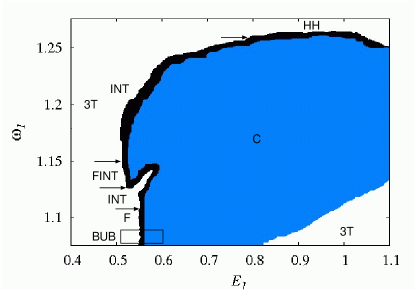
Figure 2: (Color online) Numerical phase diagram in the $(E_{1}-\omega_{1})$ plane for the circuit given in Fig. 1, represented by Eqs. (2). 3T correspond to period-3 torus, F, BUB, FINT, INT, and HH denote the birth of SNAs through gradual fractalization, bubbling, fractalization followed by intermittency, intermittency and Heagy-Hammel routes, respectively. C corresponds to the chaotic attractor. Arrows indicate the transition regions between two different types of routes to SNA.

III Two parameter Phase diagram

The parameter space of the amplitude of the external forcing $E_{1}$ and the frequency $\omega_{1}$ of the sinusoidal forcing is scanned first numerically in the range of $E_{1}\in(0.4,1.1)$ and $\omega_{1}\in{(1.075,1.275)}$ to pinpoint different dynamical behaviors and more specifically for the occurrence of SNAs through different routes. From this analysis, various dynamical transitions are determined as a function of the amplitude of the external forcing $E_{1}$ and its frequency $\omega_{1}$. Further, these dynamical behaviors and their transitions are also confirmed experimentally for the corresponding values of the experimental parameters of the circuit given in Fig. 1.

III.1 Numerical analysis

To start with, we first demarcate the parameter space $(E_{1},\omega_{1})$, by numerically integrating Eqs. (2), into quasiperiodic, strange nonchaotic and chaotic regimes by using the various qualitative and quantitative measures as discussed in the Appendix A. The numerical phase diagram is shown in Fig. 2 for $E_{1}\in(0.4,1.1)$ and $\omega_{1}\in{(1.075,1.275)}$. The various dynamical behaviors indicated in the phase diagram (Fig. 2) and the interesting dynamical transitions are elucidated in the following.

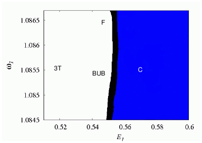
Figure 3: (Color online) Blow up picture of Fig. 2 in the bubbling transition regime indicated as BUB.

Transitions from quasiperiodic attractor to SNA and subsequently to chaotic attractor occur on increasing the value of the amplitude of the sinusoidal force $E_{1}$ for fixed value of its frequency $\omega_{1}$. Strange nonchaotic attractors created through different mechanisms are found to occur for different values of the frequency $\omega_{1}$ of the sinusoidal force. Now, we will outline the ranges of values of the frequency $\omega_{1}$ for which SNAs arise from quasiperiodic attractors through different mechanisms on increasing the value of the amplitude $E_{1}$ of the sinusoidal force.

Strange nonchaotic attractor created through the newly proposed route, namely the bubbling route, is identified in the range of frequency $\omega_{1}\in(1.085,1.086)$. Here bubbles appear in the strands of period-3 torus and then the bubbles get increasingly wrinkled in the range of the amplitude $E_{1}\in(0.54,0.55)$ of the sinusiodal forcing resulting in SNA. This phenomenon is named as the bubbling transition to SNA and it is denoted as BUB in Fig. 2. A blow up of the two parameter space corresponding to the bubbling transition is shown in Fig. 3. Further increase in the value of $E_{1}$ ends up in the chaotic behavior indicated as C in Figs. 2 and  3. Strange nonchaotic attractor created through gradual fractalization (F) of period-3 (3T) quasiperiodic attractor is identified for $\omega_{1}\in(1.086,1.111)$ as a function of the amplitude $E_{1}\in(0.5,0.55)$. Intermittency route (INT) is found to be exhibited in the range of frequency $\omega_{1}\in(1.111,1.1268)$ on increasing $E_{1}$ in the range $E_{1}\in(0.5,0.55)$ and also for $\omega_{1}\in(1.1512,1.2615)$ when $E_{1}\in(0.5,0.8)$. When the frequency $\omega_{1}\in(1.1268,1.1512)$, gradual fractalization is followed by intermittency phenomenon on increasing the value of the amplitude of the external forcing $E_{1}$. It is marked as (FINT) in Fig. 2. Torus doubling bifurcation from a period-3 torus (3T) to a period-6 (6T) torus and then to SNA via the Heagy-Hammel (HH) mechanism is found to occur in the range of $\omega_{1}\in(1.2501,1.2615)$ on decreasing $E_{1}$ in the range $E_{1}\in(1.1,0.8)$. The transition regions between the above mentioned dynamical regimes are indicated by arrows in Fig. 2 which are fixed by scanning the frequency $\omega_{1}$ of the sinusoidal force at its fourth decimal place. However, we do not draw a distinct boundary between any two scenarios because it requires a much detailed numerical analysis on a finer parameter scale.

III.2 Experimental investigation

It has additionally been confirmed that the above dynamical behaviors are also exhibited by the experimental circuit for the corresponding values of the circuit parameters $E_{f1}(=V\cdot E_{1})$ and $\omega_{f1}(=\sqrt{(C/L)}\cdot\omega_{1})$ by examining the two dimensional projections of the corresponding attractors obtained by measuring the voltage $v$ across the capacitor $C$ and the current $i_{L}$ through the inductor $L$ which are connected to the $X$ and $Y$ channels of an oscilloscope, respectively. Here $V$ is the break voltage. Then, a live picture of the corresponding power spectrum obtained from a digital storage oscilloscope (HP 54600 series) of the projected attractor has also been used to distinguish the different attractors. In addition to this, the experimental data of the corresponding attractors recorded using a 16-bit data acquisition system [AD12-16U(PCI)EH] at the sampling rate of 200 kHz have been analyzed quantitatively using the different quantification measures, namely the spectral distribution function and the distribution of finite time Lyapunov exponents. This information is then utilized (i) to pinpoint the different dynamical behaviors, (ii) to distinguish the SNAs created through different mechanisms and (iii) also to compare them with the results of numerical simulation. In the following, we will describe only the novel bubbling transition in detail by both numerical simulation and experimental realization, while the results of other known routes will be published elsewhere.

IV Bubbling route to SNA: Numerical Analysis

As noted above, in this new route, the bubbles appear in the strands of the torus as the value of the amplitude $E_{1}$ of the sinusoidal forcing is increased for a fixed value of its frequency $\omega_{1}$. The sizes of the bubbles increase further on increasing the amplitude $E_{1}$ and the bubbles increasingly get wrinkled (while the remaining parts of the strands of the torus outside the bubbles remain largely unaffected) resulting in the birth of SNA. This bubbling route is observed in the rather narrow range of frequency $\omega_{1}\in(1.085,1.086)$ as a function of the amplitude of the sinusoidal forcing $E_{1}\in(0.5,0.55)$ indicated as BUB in Figs. 2 and  3. It is to be noted that this route is significantly different from the well known fractalization route Nishikawa and Kaneko (1996), where the entire strands of the n-period torus will continuously deform and get extremely wrinkled as a function of the control parameter. The formation of SNA through this novel bubbling route has been identified in the literature for the first time to the best of our knowledge. We have used both qualitative and quantitative measures, which are indicated in the Appendix A, to confirm the new route. The qualitative proof is given through the Poincaré surface of section by distinguishing geometrically between quasiperiodic attractors and SNAs. The quantitative confirmation is provided using three different measures: (i) The largest Lyapunov exponents and its variance are used to distinguish between torus and SNA, and SNA and chaotic attractors. (ii) Scaling laws deduced from the distribution function for quasiperiodic attractors and SNAs are used to distinguish them. (iii) Finally, different routes to SNAs are also distinguished by the different distributions of local Lyapunov exponents. More information on the characterization is given in the Appendix A. In the following we provide details of the confirmation of the bubbling route.

Figure 4: Projection of the numerically simulated Poincaré surface of section of the attractors of Eqs. (2) in the $(\phi,x)$ plane for a fixed value of the frequency of the sinusoidal forcing, $\omega_{1}=1.0852$, as a function of its amplitude $E_{1}$ indicating the transition from quasiperiodic attractor to SNA through bubbling route: (a) period-3 torus (3T) for $E_{1}=0.5$, (b) bubbled strands of period-3 torus (3T) for $E_{1}=0.52$, (c) enlarged bubbles in the strands of period-3 torus (3T) for $E_{1}=0.54$, (d) fractalized bubbles for $E_{1}=0.546$ with the remaining parts (away from bubble) of the strands unaffected and (e) chaotic attractor (widely interspersed bubbles) for $E_{1}=0.56$.

Figure 5: Enlarged figures of Figs. 4 to show the bubbling transition to strange nonchaotic attractor.

IV.1 Poincaré surface of section plots and power spectra

We have fixed the value of the frequency of the sinusoidal forcing as $\omega_{1}=1.0852$ for illustration and varied its amplitude in the range $E_{1}\in(0.5,0.55)$ to elucidate the emergence of bubbling route to SNA in the present system (2). The Poincaré surface of section plot of the three strands corresponding to period-3 torus for the value of $E_{1}=0.5$ is shown in Figs. 4a and 5a. The corresponding phase portrait and power spectrum are depicted in Figs. 6a(i) and 6a(ii), respectively. As the value of the amplitude $E_{1}$ is increased further, bubbles start to appear in all the three strands starting from $E_{1}=0.516$. These are shown in Figs. 4b and 5b for $E_{1}=0.52$ and the corresponding phase portrait and power spectrum are shown in Figs. 6b(i) and 6b(ii), respectively. Further increase in the value of $E_{1}$ results in an increase in the size of the bubbles as shown in Figs. 4c and 5c for the value of $E_{1}=0.54$, whose phase portrait and power spectrum are shown in Figs. 6c(i) and 6c(ii), respectively. Beyond the value of $E_{1}=0.54$, the strands of bubbles deform and get increasingly wrinkled (while the other parts of the strands of period-3 torus outside the bubbles remain unaltered as seen in Fig. 5d) leading to the formation of SNA as depicted in Fig. 4d for the value of $E_{1}=0.546$. The phase portrait and power spectrum for this value of $E_{1}$ are shown in Figs. 6d(i) and 6d(ii), respectively. Finally, to confirm that the SNA transits to a chaotic attractor beyond $E_{1}=0.55$, we have depicted the Poincaré surface of section of the latter in Figs. 4e and 5e with the corresponding attractor and power spectrum in Figs. 6e for $E_{1}=0.56$.

The mechanism for the bubbling route is that the quasiperiodic orbit becomes increasingly unstable in its transverse direction as a function of the control parameter $(E_{1})$, resulting in the formation of the doubled strands (bubbles), as seen in Figs. 4b and 5b, in certain parts of the main strands. This instability of the quasiperiodic attractor arises due to the presence of the square wave pulse (finite amplitude for finite durations). Further increase in the value of the amplitude of the forcing $(E_{1})$ results in an increase in the size of the doubled strands (bubbles) as shown in Figs. 4c and 5c, and then the doubled strands become extremely wrinkled (without a complete doubling of the entire main strand) resulting in the SNA as depicted in Figs. 4d and 5d.

We now provide quantitative confirmation of the above results to distinguish between torus and SNA, and SNA and chaos.

Figure 6: Projection of the numerically simulated attractors and their power spectrum of Eqs. (2) for the same values of the frequency $\omega_{1}$ and the amplitude $E_{1}$ of the sinusoidal forcing as in Figs. 4. (a) period-3 torus (3T), (b) bubbled period-3 torus, (c) period-3 torus with enlarged bubbles, (d) fractalized bubbles (SNA) and (e) chaotic attractor : (i) phase portrait in the $(x,y)$ space; (ii) power spectrum.

IV.2 Largest Lyapunov exponent and its variance

The largest Lyapunov exponent, $\Lambda$, and its variance, $\mu$, that is the variance of $\Lambda$ from finite time Lyapunov exponents $\lambda_{i}(N)$’s, $i=1,2,\cdots,M$ of length $N$, defined as

$$\mu=\frac{1}{M}\sum^{M}_{i=1}(\Lambda-\lambda_{i}(N))^{2}$$ (3)

are shown in Figs. 7 in the range of $E_{1}\in(0.54,0.546)$. The attractor depicted in Fig. 6d(i) for the value of $E_{1}=0.546$ is strange but it is nonchaotic as evidenced by the negative value of the Lyapunov exponent shown in Fig. 7a. It is also to be noted that both the Lyapunov exponents and its variance (Fig. 7b) clearly indicate a critical value of amplitude $E_{1}^{c}=0.5432$, ($E_{1}<E_{1}^{c}$), below which torus exists and above which, ($E_{1}>E_{1}^{c}$), SNA appears. The regions of torus and SNA are clearly indicated by smooth and irregular variations, respectively, in the values of both the Lyapunov exponents $\Lambda$ and its variance $\mu$. Finally the transition of SNA into a chaotic attractor is confirmed by the change in the largest Lyapunov exponent from negative to positive values at $E_{1}^{c}=0.55$ as shown in the inset of Fig. 7a.

Figure 7: Transition from torus to SNA through bubbling route for the same value of frequency as in Figs. 4 and in the range of amplitude $E_{1}\in(0.54,0.546)$ obtained numerically. (a) Largest Lyapunov exponent ($\Lambda$) and (b) its variance ($\mu$). Inset in (a) depicts transition from SNA to chaos for $E_{1}\in(0.545,0.56)$.

IV.3 Spectral distribution function and scaling laws

In order to distinguish further whether the attractors depicted in Figs. 6 are quasiperiodic or strange nonchaotic or chaotic attractors, we proceed to quantify the changes in their power spectra. The spectral distribution function, defined as the number of peaks in the Fourier amplitude spectrum larger than some value $\sigma$, is used to distinguish between quasiperiodic attractors and SNA as well as SNAs and chaotic attractors. The quasiperiodic attractors obey a scaling relationship $N(\sigma)\sim\log_{10}(1/\sigma)$, while the SNAs satisfy a scaling power-law relationship $N(\sigma)\sim\sigma^{-\beta},1<\beta<2$ Romeiras and Ott (1987). Similarly for the chaotic attractor, the scaling relation is $N(\sigma)\sim\sigma^{-\beta},\beta>2$. Spectral distribution functions (filled circles) of the torus (Fig. 6a) and bubbled torus (Fig. 6b) satisfy the scaling relation $N(\sigma)\sim\log_{10}(1/\sigma)$ as indicated by the solid line in Figs. 8a and 8b, respectively, which is the characteristic of a torus. On the other hand the spectral distribution function of the SNA (Fig. 6d) exhibits power-law behavior as depicted in Fig. 8c (filled circles) with the value of the exponent $\beta=1.88$, confirming the existence of SNA. For the chaotic attractor (Fig. 6e), the scaling exponent (Fig. 8d) turns out to be $\beta=3.5$ as required. Again the solid lines in Figs. 8c and 8d represent the scaling law for SNA and chaos, respectively.

Figure 8: Spectral distribution function (filled circles) calculated numerically. (a) torus (Fig. 6a), (b) bubbled torus (Fig. 6b), (c) SNA (Fig. 6d) and (d) chaotic attractor (Fig. 6e). Solid lines in (a) and (b) corresponds to the scaling relation $N(\sigma)\sim\log_{10}(1/\sigma)$ and in (c) and (d) correspond to the scaling relation $N(\sigma)\sim\sigma^{-\beta}$, with$~{}\beta=1.88$ and $3.5$, respectively.

IV.4 Distribution of local Lyapunov exponents

In addition to the qualitative discussion through the Poincaré surface of section plots in the ($\phi,x$) plane (Figs. 4 and 5) in distinguishing the type of route through which SNA appears, it is also possible to distinguish the same using the distribution of a quantitative measure, namely finite time Lyapunov exponents. It has been shown  Prasad et al. (1997) that a typical trajectory on a SNA actually possesses positive Lyapunov exponents in finite time intervals, although the asymptotic exponent is negative. As a consequence, it is possible to observe different characteristics of SNAs created through different mechanisms by a study of the differences in the distribution of finite time exponents $P(N,\lambda)$ Prasad et al. (1997). The distribution can be obtained by taking a long trajectory and dividing it into segments of length $N$, from which the local Lyapunov exponent can be calculated. In the limit of large $N$, this distribution will collapse to a $\delta$ function $P(N,\lambda)\rightarrow\delta(\Lambda-\lambda)$. The deviations from$-$and the approach to$-$the limit can be very different for SNAs created through different mechanisms Prasad et al. (1997).

Figure 9: Distribution of finite time Lyapunov exponent calculated from both numerical data (solid line) and experimental data (dashed line) of (a) torus (Fig. 6a) and (b) SNA (Fig. 6d).

We have calculated the distribution of local Lyapunov exponents $P(N,\lambda)$, for $N=2000$, for the attractors shown in Figs. 6a(i) and 6d(i) in order to confirm the nature of transition to SNA. The distribution of the local Lyapunov exponents for the period-3 torus (solid line) is shown in Fig. 9a in which the local Lyapunov exponents are peaked about the largest Lyapunov exponents (negative values) of the torus while that of the SNA shown in Fig. 9b by solid line has its maximum at a positive value of the local Lyapunov exponents. The distribution of local Lyapunov exponents for SNA exhibits an elongated tail in its negative values because of the fact that in the bubbling transition parts of the strands of period-3 torus remain unaffected even after the birth of SNA which contributes largely to the negative values. This confirms the existence of bubbling transition to strange nonchaotic attractor.

V Bubbling route to SNA: Experimental confirmation

As a next step, in order to confirm the results of our numerical simulation in the experimental circuit shown in Fig. 1, a snapshot of the dynamical behavior for the corresponding values of the experimental parameters is obtained (as mentioned in Sec. II) and compared with that of the numerical results. Further, the corresponding experimental data are analyzed using various quantification measures mentioned in the previous section to confirm the nature of the dynamical behavior.

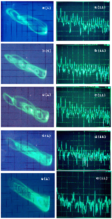
Figure 10: Snapshots of the experimental attractors and their power spectrum of the circuit shown in Fig. 1 for the corresponding values of the frequency $\omega_{f1}$ and the amplitude $E_{f1}$ of the sinusoidal forcing in Fig. 4. (a) period-3 torus (3T), (b) bubbled period-3 torus, (c) period-3 torus with enlarged bubbles, (d) fractalized bubbles (SNA) and (e) chaotic attractor: (i) phase portrait in the $(v_{C},i_{L})$ space; (ii) power spectrum.

V.1 Phase portraits and power spectra

We have depicted the snapshots of the phase portraits and the corresponding power spectra of the attractors as seen in the oscilloscope (which is connected to the circuit shown in Fig. 1) in Fig. 10 for the corresponding values of the parameters of numerical simulation. Experimental period-3 torus and its power spectrum corresponding to the numerical results, Figs. 6a, are shown in Figs. 10a(i) and 10a(ii). The attractors in the bubbling regime for the values of the amplitude of the sinusoidal forcing $E_{f1}=0.26V$ and $0.27V$ are shown in Figs. 10b(i) and c(i), respectively. The corresponding power spectra are shown in Figs. 10b(ii) and c(ii), respectively. Experimental phase portrait of the strange nonchaotic attractor and its power spectrum for the value of $E_{f1}=0.273V$ are depicted in Figs. 10d(i) and 10d(ii), respectively. It is also seen that the spectra of the quasiperiodic attractors are concentrated at a small discrete set of frequencies while the spectrum of the SNA has a much richer set of harmonics. Further the resemblance of the attractors illustrated in Figs. 10(i) with that of the attractors in Figs. 6(i) confirms the existence of bubbling transition to SNA in this negative conductance series LCR circuit with diode having both the sinusoidal and nonsinusoidal forces as quasiperiodic forcings. Finally, the chaotic attractor for $E_{f1}=0.28V$ and its power spectrum are shown in Figs. 10e.

V.2 Spectral distribution function and scaling laws

In order to confirm that the experimental phase portraits shown in Figs. 10a, 10b, 10d and 10e are indeed that of torus, bubbled torus, SNA and chaotic attractor, respectively, the corresponding data are examined for the behavior in their spectral distribution. Figs. 11a and 11b show the spectral distribution function (filled triangles) for the torus in Figs. 10a and 10b satisfying the scaling relation $N(\sigma)\sim\log_{10}(1/\sigma)$ as indicated by the solid lines while that of the SNA (Fig. 10d) shown in Fig. 11c obey power-law distribution with the value of the exponent $\beta=1.96$ lying within the characteristic value for SNAs. For the chaotic attractor (Fig. 10e), the scaling exponent turns out to be $\beta=4.0$ (Fig. 11d) as expected.

V.3 Local Lyapunov exponents

Further, in order to examine whether the SNA shown in Fig. 10d arises from the bubbling transition, the distribution of the local Lyapunov exponents calculated from the experimental data of the torus (Fig. 10a) and the SNA (Fig. 10d) are depicted in Figs. 9a and 9b respectively as dashed lines. The elongated tail in the distribution of the local Lyapunov exponents even for SNA (Fig. 10d) confirms the existence of undisturbed strands as shown in Fig. 4d, thereby confirming experimentally the birth of SNA via the bubbling transition.

Figure 11: Spectral distribution function (filled triangles) calculated from the experimental data of (a) torus (Fig. 10a), (b) bubbled torus (Fig. 10b), (c) SNA (Fig. 10d) and (d) chaotic attractor (Fig. 10e). Solid curve/line in (a) and (b) correspond to the scaling relationship for the quasiperiodic attractors and in (c) and (d) correspond to the scaling relation for the SNA and chaotic attractor, respectively.

VI Summary and conclusion

In this paper, we have reported the birth of strange nonchaotic attractors through a novel route which we term as the bubbling route to SNA in a negative conductance series LCR circuit with the diode containing nonsinusoidal (square wave) force as one of the quasiperiodic forcings. At first, we have presented the numerical analysis of the dynamical system, namely Eq. (1) of the circuit (Fig. 1) for suitable ranges of the amplitude $E_{1}$ and the frequency $\omega_{1}$ of the sinusoidal force while the other parameters are held fixed. Following this, we have also confirmed the numerical results experimentally by the snapshots of the phase portraits of the quasiperiodic attractors and SNAs as well as chaotic attractors for the corresponding values of the circuit parameters. Further, the numerical and experimental data have been analyzed using various quantification measures attributing to the existence of torus, SNA, birth of SNA through the bubbling route and transition to chaos. In particular, we have characterized the quasiperiodic attractors, SNAs and chaotic attractors using maximal Lyapunov exponent and its variance, Poincaré maps, Fourier amplitude spectra, spectral distribution function and distribution of finite time Lyapunov exponents. The distribution of local Lyapunov exponents indeed clearly distinguishes the characteristic properties of both the torus and the SNA, confirming the existence of bubbling route to the SNA. The experimental observations, numerical simulations and characteristic analysis showed that the simple dissipative negative conductance series LCR circuit even with a nonsinusoidal (square wave) force as one of the quasiperiodic forces does indeed admit strange nonchaotic behaviors of different types and in particular admits a novel bubbling route to SNA.

Appendix A Identification and characterization of SNAs and their routes

Torus, SNA and chaotic attractors and the transitions between them through different routes can be identified and characterized through various qualitative and quantitative measures. In this Appendix, we summarize the main measures used in the recent literature Venkatesan et al. (2000); Venkatesan and Lakshmanan (1997); Prasad et al. (1997); Venkatesan and Lakshmanan (2001); Zhou and Chen (1997); Kim and Lim (2004); Kapitaniak et al. (1997); Yang and Bilimgut (1997); Venkatesan et al. (1999); Ditto et al. (1990); Thamilmaran et al. (2006) in the analysis of transitions to SNAs from torus attractors and from SNAs to chaotic attractors. In the present work also, we utilize these measures.

1. Qualitative measures:
   

   Geometrically smooth (torus) and non-smooth (SNAs and chaotic) attractors can be distinguished qualitatively using Poincaré surface of sections and Fourier spectra. The Poincaré surface of section shows smooth strands for quasiperiodic attractors, non-smooth strands for SNAs, widely interspersed points throughout the phase space for chaotic attractors, which clearly reveals whether an attractor possesses a geometrically smooth or complicated structure. The spectra of the quasiperiodic attractors are concentrated at a small discrete set of frequencies while the spectra of SNAs and chaotic attractors have a much richer set of harmonics.

   Further, different types of routes to SNAs and their mechanisms for their formation can also be identified qualitatively using the Poincaré surface of sections by observing the nature of the dynamics in these plots as a function of the control parameter. Different routes for the formation of SNAs have different characteristic dynamics in their Poincaré surface of section.

2. Quantative measures:

   1. The largest Lyapunov exponents can be used to distinguish between (i) torus and SNAs and (ii) SNAs and chaotic attractors. Torus motion is characterized by a smooth negative Lyapunov exponent, SNAs are characterized by either zero or non-smooth negative Lyapunov exponents as a function of control parameters and chaotic attractors have atleast one positive Lyapunov exponent. Further, the transition from torus to SNAs exhibits different signatures in the values of the largest Lyapunov exponents and their variance for different routes to SNAs Venkatesan and Lakshmanan (2001).

   2. Further, torus and SNA can also be distinguished quantitatively by using the spectral distribution function, which is defined as the number of peaks in the Fourier amplitude spectrum larger than some value $\sigma$ Bondeson et al. (1985). The quasiperiodic attractors obey a scaling relationship $N(\sigma)\sim\log_{10}(1/\sigma)$, while the SNAs satisfy a scaling power-law relationship $N(\sigma)\sim\sigma^{-\beta},1<\beta<2$. For chaos, the scaling exponent $\beta>2$.

   3. Finer distinction between the different types of routes for the formation of SNAs can also made using the distribution of finite time Lyapunov exponents. Different routes are characterized by different types of the distribution of finite time Lyapunov exponents Prasad et al. (1997).

The different signatures of the above quantitative measures corresponding to different scenarios (routes) for the formation of three well known types of SNAs are tabulated in Table II.

Table 2: Different signatures of the largest Lyapunov exponents and its variance, and the distribution of finite time Lyapunov exponents for the formation of three prominent types of SNAs

Type of route	Lyapunov exponent $\Lambda$	Variance $\mu$	Distribution of finite time
			Lyapunov exponents $P(N,\lambda)$
Heagy-Hammel Heagy and Hammel (1994)	Irregular in the SNA region and	Small in torus	Distribution shifts continuously to
	smooth in the torus region	and large in SNA	larger exponents but the shape differs
			for torus and SNA
Gradual	Increases slowly during the	Increases only slowly	Distribution shifts continuously to
fractalization Nishikawa and Kaneko (1996)	transition from torus to SNA		larger exponents but the shape
			remains the same for torus and SNA
IntermittencyPrasad et al. (1997); Venkatesan et al. (1999)	Abrupt change during the	Abrupt change at the	Stretched exponential tail and
	transition from torus to SNA	transition point	asymmetric distribution

References

- Grebogi et al. (1984) C. Grebogi, E. Ott, S. Pelikan, and J. A. Yorke, Physica D 13, 261 (1984).
- Romeiras and Ott (1987) F. J. Romeiras and E. Ott, Phys. Rev. A 35, 4404 (1987); F. J. Romeiras, A. Bondeson, E. Ott, T. M. Andonsen, Jr., and C. Grebogi, Physica D 26, 277 (1987).
- Bondeson et al. (1985) A. Bondeson, E. Ott, and T. M. Antonsen, Jr., Phys. Rev. Lett. 55, 2103 (1985); Y. C. Lai, Phys. Rev. E 53, 57 (1996).
- Ding et al. (1989) M. Ding, C. Grebogi, and E. Ott, Phys. Rev. A 39, 2593 (1989); M. Ding and J. A. Scott Relso, Int. J. Bifurcation and Chaos Appl. Sci. Eng. 4, 533 (1994).
- Heagy and Ditto (1991) J. F. Heagy and W. L. Ditto, J. Nonlinear Sci. 1, 423 (1991); J. I. Staglino, J. M. Wersinger, and E. E. Slaminka, Physica D 92, 164 (1996).
- Yalcinkaya and Lai (1996) T. Yalcinkaya and Y. C. Lai, Phys. Rev. Lett. 77, 5039 (1996).
- Kapitaniak and Wojewoda (1993) T. Kapitaniak and J. Wojewoda, Attractors of Quasiperiodically Forced Systems (World Scientific, singapore, 1993).
- Venkatesan et al. (2000) A. Venkatesan, M. Lakshmanan, A. Prasad, and R. Ramaswamy, Phys. Rev. E 61, 3641 (2000).