Smoothing out Negative Tension Brane

Abstract

We propose an extension of the five dimensional gravitational action with an external source in order to allow arbitrary smoothing of the negative tension brane in the Randall-Sundrum model. This extended action can be derived from a model with an auxiliary four form field coupled to the gravity. We point out a further generalization of our model in relation to tachyon condensation. A possible mechanism for radion stabilization in our model is also discussed.

OU-HET-614/2008
SNUTP08-010
UT-Komaba/08-19
RIKEN-TH-100

1 Introduction

The huge hierarchy between the weak and Planck scales has been one of the most important issues in the theory of elementary particles. The braneworld with the warped compactification, which is proposed by Randall and Sundrum, is an attractive model to explain the hierarchy between the weak and Planck scales [1]. Even though the hierarchy problem is resolved in the Randall-Sundrum scenario, we still need a fine tuning among the bulk cosmological constant and the brane tensions in order to acquire the observed four-dimensional cosmological constant $\Lambda_{4}\lesssim 10^{-120}M_{P}^{4}$, where $M_{P}$ is the four-dimensional Planck scale determined by the Newton’s law of gravitation in four dimensions. This fine tuning requires that one of the branes should have a negative tension. Although the negative tension brane appears to lead to some pathology in general relativity [2] (see also [3]), detailed analyses have revealed that the four-dimensional effective theory on the negative tension brane can be consistent with the standard Einstein gravity [4, 5] as far as the moduli for the compactification radius, the radion, is fixed by some mechanism, such as the one proposed by Goldberger and Wise [6].

Recent progress in string theory has revealed that the compactified space is generically warped under the presence of background fluxes [7], and much effort to realize Randall-Sundrum scenario in superstring theory has been made, see e.g. [8] and references therein. The realization of Randall-Sundrum scenario in superstring theory naturally requires the supersymmetric extension of the Randall-Sundrum model in five-dimensional effective supergravity.

So far, two ways to supersymmetrize the Randall-Sundrum model are proposed in [9, 10] and in [11], respectively. The former involves a kinky gauge coupling which has position dependence like a step function in the extra dimension. Especially the multiple of the step function and its derivative, the delta function, vanishes everywhere. The latter does not involve the position dependent gauge coupling but it implicitly assumes that the multiple of a step function and a delta function takes a finite non-zero value on the branes [12, 13].

We want to have a way to regularize, i.e. smooth out, the step function and the delta function in the Randall-Sundrum geometry in particular on the brane. The step function would be realized as a kink solution of a bulk field. The positive tension brane has been smoothed out by introducing a bulk scalar field with solitonic kink solutions [14]. It has been shown that the negative tension brane cannot be smoothed by a bulk scalar field without an instability of the spacetime [15, 16, 17, 18].

Here we propose an extension of the five-dimensional Einstein-Hilbert action that allows the smoothing of the negative tension brane. In our regularized model, the multiple of the step function and the delta function vanishes on the branes in the singular limit, in agreement with [9, 10]. Our model might provide an insight on the supersymmetrization of the Randall-Sundrum model without resorting to singular configurations.

Besides the somewhat technical motivation presented above, our study can be placed on more general physical ground. Singular objects such as D-branes in string theory are often interpreted as solitonic smooth objects in dynamical or quantum mechanical analysis. Our regularization could be a useful tool for these analyses in the braneworld models.

In the next section, we describe our model of the extension of five-dimensional Einstein gravity. In Section 3, we present a possible embedding of our model into the standard five-dimensional gravity with a four-form field. Further extension with a coupling between the four-form and a scalar source is also shown, inspired by the tachyon condensation in string theory. In Section 4, we show that the radion can be stabilized by a natural extension of the Goldberger-Wise mechanism. In the last section, we provide summary and discussions.

2 Modified Gravitational Action

Let us first briefly review the Randall-Sundrum model [1]. The fifth dimension $y$ is compactified on $S^{1}/Z_{2}$ by the identifications $y\sim y+2L$ and $-y\sim y$. When we restrict it to $-L<y\leq L$, the gravitational part of the action reads

$$S_{0} ={M_{*}^{3}}\int d^{5}x\sqrt{-g}\left({R\over 2}-\Lambda-\lambda_{0}\delta(y)-\lambda_{L}\delta(y-L)\right),$$ (1)

where $M_{*}^{3}=1/8\pi G$ with $G$ being the higher dimensional Newton constant. Note that this action does not have the full five-dimensional diffeomorphism invariance, but the only four-dimensional diffeomorphism invariance and reparametrization invariance with respect to the compact direction $y$.

The Randall-Sundrum geometry is a slice of the five dimensional anti de Sitter space (AdS₅):

$$ds^{2} =e^{-2k|y|}\eta_{\mu\nu}dx^{\mu}dx^{\nu}+dy^{2},$$ (2)

where $k$ is its curvature scale. The metric (2) becomes a solution to the five dimensional Einstein equation $\delta S/\delta g^{MN}=0$ if the five dimensional bulk cosmological constant $\Lambda$ and the brane tensions $\lambda_{0}$ and $\lambda_{L}$ are fine-tuned to be

$$\Lambda=-k\lambda_{0}=k\lambda_{L}=-6k^{2}<0.$$ (3)

Physically the condition (3) implies that the ultraviolet (UV) brane at $y=0$ has the positive tension while the infrared (IR) brane at $y=L$ has the negative one. In [14] it has been shown that the positive tension brane can be smoothed out by introducing a bulk scalar having a kink profile.

There have been attempts to smooth out the negative tension brane by introducing a so-called ghost scalar, which is a propagating degree of freedom having a wrong-sign kinetic term [15, 16, 17]. Obviously there are resulting difficulties both at the classical and quantum levels. Here we attempt to smooth out the negative tension brane in a different way. A possible resolution to the wrong sing kinetic term is shown in the next section.

Now we propose a modification of the action (1) preserving the same symmetry, that is the four dimensional diffeomorphisms and the reparametrization of the fifth coordinate $y$:

$$S_{g} =M_{*}^{3}\int d^{5}x\sqrt{-g}\left({R\over 2}-\Lambda\varepsilon(y)^{2}-\lambda{\varepsilon^{\prime}(y)\over 2\sqrt{g_{yy}}}\right),$$ (4)

where $\varepsilon(y)$ is an arbitrary $Z_{2}$ odd periodic function:

$$\varepsilon(y+2L) =\varepsilon(y), \varepsilon(-y) =-\varepsilon(y),$$ (5)

and $\varepsilon^{\prime}(y)=\partial_{y}\varepsilon(y)$.

If we again fine tune the cosmological constant and the brane tension:

$$\Lambda=-k\lambda=-6k^{2}<0,$$ (6)

the Einstein equation

$$R_{MN}-{g_{MN}\over 2}R+\Lambda\varepsilon(y)^{2}g_{MN}+\lambda{\varepsilon^{\prime}(y)\over 2\sqrt{g_{yy}}}\left(g_{MN}-{g_{yM}g_{yN}\over g_{yy}}\right) =0$$ (7)

has a solution:

$$ds^{2}=e^{-2\sigma(y)}\eta_{\mu\nu}dx^{\mu}dx^{\nu}+dy^{2},$$ (8)

where

$$\sigma(y) =k\int^{y}d\tilde{y}\,\varepsilon(\tilde{y}).$$ (9)

We note that the equation of motion of $\varepsilon(y)$:

$$2\Lambda\varepsilon(y)=\frac{\lambda}{2\sqrt{-g}}\partial_{y}\left(\frac{\sqrt{-g}}{\sqrt{g_{yy}}}\right),$$ (10)

is automatically satisfied due to Eqs. (6) and (9).

Now we can have an arbitrary shape of the $Z_{2}$ even periodic function $\sigma(y)$ by a proper choice of $\varepsilon(y)$. A choice of the external source $\varepsilon(y)$ gives a corresponding gravitational action. Any choice of $\varepsilon(y)$ can satisfy the Einstein equation as well as the equation of motion of $\varepsilon(y)$ itself, with the tuning (6). One might wonder what is the source of such a large symmetry. We come back to this point in the next section.

When we take $\varepsilon(y)$ to be the step function:

$$\varepsilon(y) =\begin{cases}1&(0<y<L),\\ -1&(-L<y<0),\end{cases}$$ (11)

we recover the original setup (1) with $\lambda=\lambda_{0}=-\lambda_{L}$. The point here is that a continuous deformation of the negative tension brane becomes possible. For instance, we can take

$$\varepsilon(y) =-\tanh[\beta(y+L)]+\tanh\beta y-\tanh[\beta(y-L)]$$ (12)

for $-L\leq y\leq L$. In the $\beta\to\infty$ limit, $\varepsilon(y)$ in (12) goes back to the step function (11). For (12), the $\sigma(y)$ is obtained as

$$\sigma(y) ={k\over\beta}\log{\cosh\beta y\over\cosh[\beta(y-L)]\cosh[\beta(y+L)]}+2.$$ (13)

As an example, the plot for $\beta=50$ is shown in Fig. 1. Note that this gives a smooth regularization of the Randall-Sundrum geometry which is fully consistent with the bulk Einstein equation.

Figure 1: Smoothed functions $\sigma(y)$ (left), $\varepsilon(y)=\sigma^{\prime}(y)/k$ (center), and $\varepsilon^{\prime}(y)$ (right) for $\beta=50$.

In our formulation, the multiple of the (regularized) step and delta functions is always zero on the branes,

$$\varepsilon(y)\varepsilon^{\prime}(y)=0\qquad\text{at $y=0,L$}.$$ (14)

Therefore, it may be utilized as a tool to supersymmetrize the Randall-Sundrum model in the formulation of [9, 10], but not directly for [11].

3 Four Form Field and Tachyon Condensation

So far, the action (4) is given just by hand. One might consider that this is too ad hoc. Here we argue that the action (4) could be regarded as an effective theory of an underlying microscopic theory.

Let us consider the following five dimensional gravitational action coupled to a four-form gauge field $A_{4}$:

$$S ={M_{*}^{3}\over 2}\int\left(R\wedge*1+F_{5}\wedge*F_{5}\right),$$ (15)

where $F_{5}=dA_{4}$ and $*$ is the Hodge dual in five dimensions. Note that the gauge kinetic term has a wrong sign here. This does not lead to an immediate inconsistency because $A_{4}$ has no physical degree of freedom in five dimensions. Such a wrong-sign “auxiliary” gauge field has also been introduced by Turok and Hawking for an inflation model inspired by the M-theory [20].

Generically one can write a five form field in five dimensions as

$$F_{5} =f(x)\sqrt{-g}\,d^{5}x, *F_{5} =-f(x),$$ (16)

where $d^{5}x=dx^{0}\wedge\dots\wedge dx^{3}\wedge dy$ and $f(x)$ is a scalar function. The action in terms of $f(x)$ reads

$$S ={M_{*}^{3}\over 2}\int\sqrt{-g}\,d^{5}x\left(R-f^{2}\right)={M_{*}^{3}\over 2}\int\sqrt{-g}\,d^{5}x\left(R+\varphi^{2}-2\varphi f\right),$$ (17)

where we have introduced another auxiliary field $\varphi$ in the last step.

The gauge field $A_{4}$ has five independent component fields. Assuming the invariance under the four dimensional diffeomorphisms and the reparametrization of $y$, it would be natural to expect that the components of $A_{4}$ except for $A_{\mu_{1}\mu_{2}\mu_{3}\mu_{4}}$, where $\mu_{i}=0,\cdots,3$, are irrelevant, and therefore they could be ignored from the beginning. For the remaining component, we make the following field redefinition:

$$A_{4} =a(x)\sqrt{-g^{(4)}}\,d^{4}x,$$ (18)

where $a(x)$ is a scalar function and $d^{4}x=dx^{0}\wedge\dots\wedge dx^{3}$. In terms of $a(x)$, the field strength becomes

$$f ={1\over\sqrt{-g}}\partial_{y}\left(a(x)\sqrt{-g^{(4)}}\right).$$ (19)

Putting this into the action, we obtain

$$S ={M_{*}^{3}\over 2}\int d^{5}x\sqrt{-g}\left(R+\varphi^{2}+{2a(x)\over\sqrt{g_{yy}}}\partial_{y}\varphi\right),$$ (20)

where we have performed the partial integration. If we could choose $\varphi(x)$ and $a(x)$ as

$$\varphi(x) =\sqrt{\Lambda}\,\varepsilon(x), a(x) ={\lambda\over 4\sqrt{\Lambda}},$$ (21)

we recover the extended action (4).

Now it is obvious why $\varepsilon$ can be an arbitrary function, that is, why $\delta S/\delta\varepsilon=0$ is always satisfied because $\varepsilon$ is nothing but an auxiliary field $\varphi$. The fine tuning of the cosmological constant and the brane tension is done by fixing the constant value of the scalar field $a(x)$. We note that $a(x)$ must be treated as a genuinely external source, as long as the action (15) is regarded as the microscopic action of our theory, because the equation of motion for $a(x)$ leads to the unwanted condition $\varepsilon^{\prime}(y)=0$ which does not allow a kink-like solution.

It is interesting to observe that the action (15) can be rewritten as (20) which is similar to (4). There might be a more fundamental theory whose action includes the terms in (15) so that our action (4) can be regarded as (a part of) its effective action. Then the resultant equation of motion of $a(x)$ would be more complicated, hopefully allowing a non-trivial solution for $\varphi(x)$. The constant $a(x)$ solution should be consistent with the equations of motion of the fundamental theory.

In the more fundamental theory, the profile of $\varepsilon(y)$, which has been completely arbitrary so far, might be determined by some mechanism. For example, suppose that there is the following term of the Chern-Simons type in the action of the underlying theory:

$$S_{CS} =\int dT\wedge A_{4},$$ (22)

where $T$ is a $Z_{2}$-odd scalar source. Due to this term, the equation of motion of $a(x)$ can relate $\varphi(x)$ to $T(x)$. As a result, if $T(x)$ has a kink-like profile, so would $\varphi(x)$. Note that this term is topological, i.e. independent of metric and does not change the Einstein equation. We also note that this extra term often appears in string theory in the context of the tachyon condensation where the $T(x)$ is indeed identified as a tachyon field, see [21] for a review and references therein. Further investigation of a possible underlying theory that can lead to our action is left for future research.

4 Introducing bulk scalar field

In general a bulk scalar field plays a crucial role in the radion stabilization [6, 14]. To see the dependence on radius $L$ explicitly in our setup, we rewrite our background metric (2) as

$$ds^{2} =e^{-2kL\alpha(\theta)}\eta_{\mu\nu}dx^{\mu}dx^{\nu}+L^{2}d\theta^{2},$$ (23)

where $\alpha(\theta)=\alpha(\theta+2)$ is an arbitrary dimensionless periodic function. One can check that the equation of motion for the metric is satisfied for an arbitrary $L$, which is promoted to a massless field, radion, in the perturbation analysis.

In our setup having symmetries of four dimensional diffeomorphisms and reparametrization of the fifth coordinate, a bulk scalar field $\Phi$ can couple to the gravity in the following form

$$S =M_{*}^{3}\int d^{5}x\sqrt{-g}\left[{R\over 2}-\Lambda(\Phi)\varepsilon^{2}-\lambda(\Phi){\partial_{5}\varepsilon\over 2\sqrt{g_{55}}}-{g^{MN}\over 2M_{*}^{3}}\partial_{M}\Phi\partial_{N}\Phi\right],$$ (24)

where the cosmological constant $\Lambda$ and the brane tension $\lambda$ are now promoted to functions of $\Phi$. The mass dimensions are: $[\Phi]=3/2$, $[\Lambda]=2$, and $[\lambda]=1$. Assuming that the vacuum expectation value is much smaller than the Planck scale $\Phi^{2}\ll M_{*}^{3}$, we can expand in terms of $(\Phi^{2}/M_{*}^{3})$

$$\Lambda(\Phi) =M_{*}^{2}\left(c_{1}+{c_{2}\over 2}{\Phi^{2}\over M_{*}^{3}}+{c_{3}\over 4!}\left({\Phi^{2}\over M_{*}^{3}}\right)^{2}+\cdots\right),$$

$$\lambda(\Phi) =M_{*}\left(d_{1}+{d_{2}\over 2}{\Phi^{2}\over M_{*}^{3}}+{d_{3}\over 4!}\left({\Phi^{2}\over M_{*}^{3}}\right)^{2}+\cdots\right),$$ (25)

where we have assumed the invariance under the flip $\Phi\rightarrow-\Phi$ for simplicity.

To allow the solution of the form of the generalized step function $\varepsilon(\theta)=\alpha^{\prime}(\theta)$, we set the first order constants to be $c_{1}=-6(k/M_{*})^{2}$ and $d_{1}=6(k/M_{*})$. Note that the fine tuning of the first order constants $c_{1}$ and $d_{1}$ corresponds to the fine-tuning of the cosmological constant, which is inevitable for all the versions of Randall-Sundrum type models so far.

The resultant bulk scalar field equation is

$$\Phi^{\prime\prime}(\theta)-4kL\alpha^{\prime}(\theta)\Phi^{\prime}(\theta)-L^{2}M_{*}^{3}\left[\alpha^{\prime}(\theta)^{2}{\partial\Lambda\over\partial\Phi}+{\alpha^{\prime\prime}(\theta)\over 2L}{\partial\lambda\over\partial\Phi}\right]=0.$$ (26)

Once we find the solution to the field equation (26) for $\Phi$, generically a potential for the radion $L$ in the four-dimensional effective theory is generated as

$$V(L) =LM_{*}^{3}\int_{-1}^{1}d\theta\,e^{-4kL\alpha(\theta)}\left(\alpha^{\prime}(\theta)^{2}\Lambda(\Phi)+{\alpha^{\prime\prime}(\theta)\over 2L}\lambda(\Phi)+{1\over 2L^{2}M_{*}^{3}}\Phi^{\prime}(\theta)^{2}\right).$$ (27)

Since, in general, the equation (26) is highly non-linear, we cannot expect to have an analytic solution. However, for free scalar field, one can obtain an analytic solution for a certain choice of parameters as we show below. By an ansatz $\Phi(\theta)=v^{3/2}e^{\sigma(\theta)}$, the field equation (26) reads

$$\sigma^{\prime\prime}(\theta)+\sigma^{\prime}(\theta)^{2}-4kL\,\alpha^{\prime}(\theta)\sigma^{\prime}(\theta)-\left(LM_{*}\right)^{2}\left[c_{2}+\cdots\right]\alpha^{\prime}(\theta)^{2}-{LM_{*}\over 2}\left[d_{2}+\cdots\right]\alpha^{\prime\prime}(\theta)=0,$$ (28)

where terms denoted by $\cdots$ are $O(v^{3}/M_{*}^{3})$ and neglected in the following. The parameter $v$ becomes the vacuum expectation value of $\Phi$ at the positive tension brane in the limit (11) with the normalization $\alpha(0)=0$. Here, we set the second order constants $c_{2}={d_{2}\over 4}\left(d_{2}-{8k\over M_{*}}\right)$ so that we can have an analytic solution

$$\sigma(\theta) ={d_{2}\over 2}LM_{*}\alpha(\theta).$$ (29)

There should be a more general solution to the equation (26), since it is the second order differential equation while the solution specified by (29) has only one integration constant $v$. To examine the general solution, it is convenient to define $\Psi(\theta)=e^{-d_{2}LM_{*}\alpha(\theta)/2}\Phi(\theta)$. The equation for $\Psi(\theta)$ is reduced to

$$\Psi^{{}^{\prime\prime}}(\theta)+\left(d_{2}M_{*}-4k\right)L\alpha^{{}^{\prime}}(\theta)\Psi^{{}^{\prime}}(\theta)=0.$$ (30)

Obviously, $\Psi(\theta)=\textrm{const.}$ is a trivial solution. The above equation can be integrated easily and the general solution becomes

$$\Psi(\theta)=A+B\int^{\theta}d\tilde{\theta}\exp\left(\left(d_{2}M_{*}-4k\right)L\alpha(\tilde{\theta})\right).$$ (31)

Since the integral in the second term does not satisfy periodicity condition $\Psi(\theta+2)=\Psi(\theta)$, one has to put $B=0$. This proves that the solution (29) gives the general periodic solution to Eq. (26).

Using this solution, we have the effective potential for the radius $L$ up to quartic order ($\sim\Phi^{4}$):

$$V(L) ={Lv^{6}\over 24M_{*}}\left(c_{3}-d_{3}\tilde{d}_{2}\right)\int_{-1}^{1}d\theta\,\alpha^{\prime}(\theta)^{2}e^{2\tilde{d}_{2}LM_{*}\alpha(\theta)},$$ (32)

where we have defined $\tilde{d}_{2}\equiv d_{2}-{2k\over M_{*}}$. Note that $c_{1}$ and $d_{1}$ terms are being understood to cancel the gravitational part and hence omitted and that the quadratic $\Phi^{2}$ terms vanish too. Since all the non-linear terms are suppressed by $v^{3}/M_{*}^{3}$, our free field solution and effective potential correspond to the leading approximations in the $v^{3}/M_{*}^{3}$ expansion.

In Fig. 2, we plot the potential $V(L)$ with the regularized profile (13) for $\beta=50$ and the parameters $\tilde{d}_{2}=-1,~{}c_{3}-d_{3}\tilde{d}_{2}=-0.1$ as an illustration.

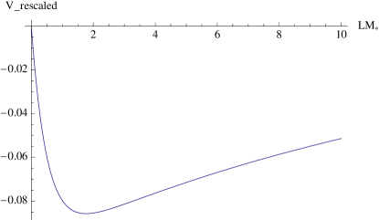
Figure 2: Sample radion potential being rescaled as $V(LM_{*})/{v^{6}\over 24M_{*}^{2}}$ vs. dimensionless redius $LM_{*}$ for parameters $\tilde{d}_{2}=-1$ and $c_{3}-d_{3}\tilde{d}_{2}=-0.1$.

We see that the non-trivial potential for $L$ is generated as the first approximation in the $v^{3}/M_{*}^{3}$ expansion. Several comments are in order:

• The resultant potential minimum value is negative here and we have to fine-tune the cosmological constant again by shifting $c_{1},d_{1},c_{2},d_{2}$.

• In the singular limit, $\alpha(\theta)\rightarrow|\theta|$, the effective potential becomes a monotonically decreasing function of $L$, and does not have a minimum. The non-trivial minimum is generated due to the smoothness of the branes.

• The original Goldberger-Wise setup [6] corresponds to $c_{3}=0$, where it has been crucial to have different (positive) brane potentials from each other. However, in our action (24), the brane potential is given by a single function $\lambda(\Phi)$ and cannot be independent of each other even in the singular limit. In particular, the sign of quartic coupling in the brane potential is flipped by the factor $\partial_{5}\varepsilon\propto\left[\delta(y)-\delta(y-L)\right]$ in the step-function limit (11) in Eq. (24), while it should be positive on the both branes in the Goldberger-Wise setup. It would also be interesting to realize the Goldberger-Wise mechanism by introducing another bulk scalar field in our setup.

• The study including the higher order non-linear terms in the equation of motion for $\Phi$ would require a detailed numerical analysis, which we leave for future research. Also, the back-reaction from $\Phi$ to the metric is neglected at this order. For a fixed four form field, we expect that gravitational instability would be absent after the stabilization of the radion. See also Refs. [23, 24, 25] for related issues.

5 Summary and Discussions

We have proposed the modification of the five dimensional gravitational action that allows an arbitrary smoothing of the negative tension brane in the context of the Randall-Sundrum I brane world. This can be viewed not only as a possible regularization but also as arising from the high energy theory with the four form auxiliary gauge field. It would be interesting to investigate possible connection of our mechanism to the four form mechanism in the five dimensional supergravity [12, 13].

The application of our regularized $Z_{2}$-odd function $\varepsilon(y)$ to the $Z_{2}$-odd graviphoton gauge coupling might be possible in the context of the supersymmetric Randall-Sundrum model [9, 10] with $\varepsilon(y)\varepsilon^{\prime}(y)=0$ on the branes, while the version [11] with $\varepsilon(y)\varepsilon^{\prime}(y)\neq 0$ would require further elaboration.

We have discussed that the profile of the four form field can arise from the tachyon condensation in string theory. In the point of view of tachyon condensation, it would be natural to expect the following scenario to be realized: The five-dimensional spacetime is filled with an unstable D-brane on which there exists a tachyon $T$. If $T$ forms a kink, then the kink would be regarded as a stable D3-brane to which $A_{4}$ couples. In other words, the braneworld is created dynamically. However, it seems strange that, in this scenario, an anit-kink corresponds to a negative-tension brane since it is usually regarded as just an anti-brane with a positive tension. It would be worth studying this issue further.

Our model does not allow the Goldberger-Wise mechanism for the radion stabilization. However we show that the introduction of the bulk scalar field and its natural embedding into our extended action can stabilize the radion. The stability under gravitational perturbation of the system would be worth investigating.

References

- [1] L. Randall and R. Sundrum, “A large mass hierarchy from a small extra dimension,” Phys. Rev. Lett. 83 (1999) 3370 [arXiv:hep-ph/9905221].
- [2] T. Shiromizu, K. i. Maeda and M. Sasaki, “The Einstein equations on the 3-brane world,” Phys. Rev. D 62 (2000) 024012 [arXiv:gr-qc/9910076].
- [3] A. N. Aliev and A. E. Gumrukcuoglu, “Gravitational field equations on and off a 3-brane world,” Class. Quant. Grav. 21 (2004) 5081 [arXiv:hep-th/0407095].
- [4] S. Kanno and J. Soda, “Radion and holographic brane gravity,” Phys. Rev. D 66 (2002) 083506 [arXiv:hep-th/0207029].
- [5] T. Shiromizu and K. Koyama, “Low energy effective theory for two brane systems: Covariant curvature formulation,” Phys. Rev. D 67 (2003) 084022 [arXiv:hep-th/0210066].
- [6] W. D. Goldberger and M. B. Wise, “Modulus stabilization with bulk fields,” Phys. Rev. Lett. 83, 4922 (1999) [arXiv:hep-ph/9907447].
- [7] S. B. Giddings, S. Kachru and J. Polchinski, “Hierarchies from fluxes in string compactifications,” Phys. Rev. D 66, 106006 (2002) [arXiv:hep-th/0105097].
- [8] F. Brummer, A. Hebecker and E. Trincherini, “The throat as a Randall-Sundrum model with Goldberger-Wise stabilization,” Nucl. Phys. B 738 (2006) 283 [arXiv:hep-th/0510113].
- [9] T. Gherghetta and A. Pomarol, “Bulk fields and supersymmetry in a slice of AdS,” Nucl. Phys. B 586, 141 (2000) [arXiv:hep-ph/0003129].
- [10] A. Falkowski, Z. Lalak and S. Pokorski, “Supersymmetrizing branes with bulk in five-dimensional supergravity,” Phys. Lett. B 491 (2000) 172 [arXiv:hep-th/0004093].
- [11] R. Altendorfer, J. Bagger and D. Nemeschansky, “Supersymmetric Randall-Sundrum scenario,” Phys. Rev. D 63 (2001) 125025 [arXiv:hep-th/0003117].
- [12] E. Bergshoeff, R. Kallosh and A. Van Proeyen, “Supersymmetry in singular spaces,” JHEP 0010 (2000) 033 [arXiv:hep-th/0007044].
- [13] T. Fujita, T. Kugo and K. Ohashi, “Off-shell formulation of supergravity on orbifold,” Prog. Theor. Phys. 106 (2001) 671 [arXiv:hep-th/0106051].
- [14] O. DeWolfe, D. Z. Freedman, S. S. Gubser and A. Karch, “Modeling the fifth dimension with scalars and gravity,” Phys. Rev. D 62 (2000) 046008 [arXiv:hep-th/9909134].
- [15] R. Koley and S. Kar, “Bulk phantom fields, increasing warp factors and fermion localisation,” Mod. Phys. Lett. A 20 (2005) 363 [arXiv:hep-th/0407159].
- [16] M. Pospelov, “Ghosts and tachyons in the fifth dimension,” Int. J. Mod. Phys. A 23 (2008) 881 [arXiv:hep-ph/0412280].
- [17] N. J. Nunes and M. Peloso, “On the stability of field-theoretical regularizations of negative tension branes,” Phys. Lett. B 623 (2005) 147 [arXiv:hep-th/0506039].
- [18] R. Koley and S. Kar, “A novel braneworld model with a bulk scalar field,” Phys. Lett. B 623 (2005) 244 [Erratum-ibid. B 631 (2005) 199] [arXiv:hep-th/0507277].
- [19] K. Oda and A. Weiler, “Wilson lines in warped space: Dynamical symmetry breaking and restoration,” Phys. Lett. B 606 (2005) 408 [arXiv:hep-ph/0410061].
- [20] N. Turok and S. W. Hawking, “Open inflation, the four form and the cosmological constant,” Phys. Lett. B 432, 271 (1998) [arXiv:hep-th/9803156].
- [21] A. Sen, “Non-BPS states and branes in string theory,” arXiv:hep-th/9904207.
- [22] C. Csaki, “TASI lectures on extra dimensions and branes,” arXiv:hep-ph/0404096.
- [23] J. L. Lehners, P. Smyth and K. S. Stelle, “Stability of Horava-Witten spacetimes,” Class. Quant. Grav. 22 (2005) 2589 [arXiv:hep-th/0501212].
- [24] D. Maity, S. SenGupta and S. Sur, “Stability analysis of the Randall-Sundrum braneworld in presence of bulk scalar,” Phys. Lett. B 643 (2006) 348 [arXiv:hep-th/0604195].
- [25] D. Maity, S. SenGupta and S. Sur, “The role of higher derivative bulk scalar in stabilizing a warped spacetime,” arXiv:hep-th/0609171.