Helioseismic data inclusion in solar dynamo models

Abstract

An essential ingredient in kinematic dynamo models of the solar cycle is the internal velocity field within the simulation domain – the solar convection zone. In the last decade or so, the field of helioseismology has revolutionized our understanding of this velocity field. In particular, the internal differential rotation of the Sun is now fairly well constrained by helioseismic observations almost throughout the solar convection zone. Helioseismology also gives us some information about the depth-dependence of the meridional circulation in the near-surface layers of the Sun. The typical velocity inputs used in solar dynamo models, however, continue to be an analytic fit to the observed differential rotation profile and a theoretically constructed meridional circulation profile that is made to match the flow speed only at the solar surface. Here we take the first steps towards the use of more accurate velocity fields in solar dynamo models by presenting methodologies for constructing differential rotation and meridional circulation profiles that more closely conform to the best observational constraints currently available. We also present kinematic dynamo simulations driven by direct helioseismic measurements for the rotation and four plausible profiles for the internal meridional circulation – all of which are made to match the helioseismically inferred near-surface depth-dependence, but whose magnitudes are made to vary. We discuss how the results from these dynamo simulations compare with those that are driven by purely analytic fits to the velocity field. Our results and analysis indicate that the latitudinal shear in the rotation in the bulk of the solar convection zone plays a more important role, than either the tachocline or surface radial shear, in the induction of the toroidal field. We also find that it is the speed of the equatorward counterflow in the meridional circulation right at the base of the solar convection zone, and not how far into the radiative interior it penetrates, that primarily determines the dynamo cycle period. Improved helioseismic constraints are expected to be available from future space missions such as the Solar Dynamics Observatory and through analysis of more long-term continuous data sets from ground-based instruments such as the Global Oscillation Network Group. Our analysis lays the basis for the assimilation of these helioseismic data within dynamo models to make future solar cycle simulations more realistic.

1 Introduction

The dynamic nature of solar activity can often be traced back to the presence and evolution of magnetic fields in the Sun. The more intense magnetic fields on the order of $1000$ Gauss (G) are observed to be concentrated within regions known as sunspots, which often appear in pairs of opposite magnetic polarities (Hale 1908). Sunspots have been observed regularly now for about four centuries starting with the telescopic observations of Galileo Galilei in the early 1600s. These observations point out that the number of sunspots on the solar surface varies in a cyclic fashion with an average periodicity of 11 years (Schwabe 1844), although there are variations both in the amplitude and period of this cycle. At the beginning of a cycle sunspots appear at about mid-latitudes in both hemispheres (with opposite polarity orientation across the hemispheres) and then progressively appear at lower and lower latitudes as the cycle progresses (Carrington 1858) until no sunspots are seen (i.e., solar minimum). In the next cycle, the same pattern repeats, but the new cycle spots have their bipolar magnetic orientation reversed relative to the previous cycle (in both hemispheres). So considering sign as well as amplitude, the solar cycle has a period of $22$ years.

There is a weaker, more diffuse component of the magnetic field outside of sunspots which is seen to have a somewhat different evolution. This field – whose radial component has been observable at the solar surface since the advent of the magnetograph – was believed to be on the order of $10$ Gauss. It is found that this field is concentrated in unipolar patches, which originate at sunspot latitudes at the time of sunspot maxima, and then moves poleward with the progress of the sunspot cycle (Babcock 1959; Bumba and Howard 1965; Howard and LaBonte 1981). The sign of this radial field of any given cycle is opposite to the old cycle polar field, which it cancels and reverses upon reaching the poles. The amplitude of this radial field achieves a maximum (at the poles) at the time of sunspot minimum (i.e. with a $90^{\circ}$ phase difference relative to the sunspots). However, the periodicity of the cycle of this field matches the sunspot cycle period, underscoring that they are related. Recent observations by Hinode indicate that this radial field gets concentrated within unipolar flux tubes with field strength on the order of $10^{3}$ Gauss (Tsuneta et al. 2008).

Explanations of this observations of the solar magnetic cycle rely on the field of magnetohydrodynamic dynamo theory, which seeks to address the generation and evolution of magnetic fields as a complex non-linear process involving interactions between the magnetic field and plasma flows within the solar interior. In particular, it is now believed that the solar cycle involves the generation and recycling (feeding on the energy available in plasma motions) of two components of the magnetic field – the toroidal component and the poloidal component. In an axisymmetric spherical coordinate system, the magnetic and velocity fields can be expressed as

$${\bf B} = B_{\phi}{\bf\hat{e}}_{\phi}+\nabla\times(A{\bf\hat{e}}_{\phi})$$ (1)

$${\bf v} = r\sin(\theta)\Omega{\bf\hat{e}}_{\phi}+{\bf v}_{p}$$ (2)

where the first term on the right hand side (R.H.S.) of Equations $1$ and $2$ is the toroidal component (in the case of the velocity field this corresponds to the differential rotation) and the second term is the poloidal component of the field (in the case of the velocity field this corresponds to the meridional circulation). The toroidal component of the magnetic field is thought to be produced by stretching of an initially poloidal field by the differential rotation of the Sun (the dynamo $\Omega$-effect); subsequently, strong toroidal flux loops rise up due to magnetic buoyancy emerging through the solar surface as sunspots (Parker 1955a). To complete the dynamo cycle, the poloidal field (whose radial component is manifested as the observed vertical field on the solar surface) has to be regenerated from this toroidal field in a process that is traditionally called the dynamo $\alpha$-effect. The first explanation of this $\alpha$-effect was due to Parker (1955b) who suggested that helical turbulent convection in the solar convection zone (SCZ) would twist rising toroidal flux tubes into the poloidal plane, recreating the poloidal component of the magnetic field. Much has changed since this pioneering description of the first solar dynamo model by Parker, although the basic notion of the recycling of the toroidal and poloidal components remain the same.

First of all, simulations of the buoyant rise of toroidal flux tubes point out that to match the observed properties of sunspots at the solar surface, the strength of these flux tubes at the base of the SCZ has to be much more than the equipartition field strength of $10^{4}$ G (D’Silva & Choudhuri 1993; Fan, Fisher & DeLuca 1993). The classical dynamo $\alpha$-effect due to helical turbulence is expected to be quenched for super-equipartition field strengths and therefore other physical processes have to be invoked as a regeneration mechanism for the poloidal field. One of the alternatives is an idea originally due to Babcock (1961) and Leighton (1969). The Babcock and Leighton (hereby BL) model proposes that the decay and dispersal of tilted bipolar sunspot pairs at the near-surface layers, mediated by diffusion, differential rotation, and meridional circulation, can regenerate the poloidal field. This mechanism is actually observed and is simulated as a surface flux transport process that can reproduce the solar polar field reversals (Wang, Nash & Sheeley 1989). Therefore a synthesis of Parker’s original description along with the BL mechanism for poloidal field generation is now widely accepted as a leading contender for explaining the solar dynamo mechanism (Choudhuri, Schüssler & Dikpati 1995; Durney 1997; Dikpati & Charbonneau 1999; Nandy & Choudhuri 2001; Nandy 2003), although there are other alternative suggestions as well. A description of all of those is beyond the scope of this paper and interested readers are referred to the review by Charbonneau (2005).

Second, helioseismology has now mapped the solar internal rotation profile (Schou et al. 1998; Charbonneau et al. 1999), which is observed to be vary mainly in the latitudinal direction in the main body of the SCZ. Helioseismology has also discovered the tachocline – a region of strong radial and latitudinal shear beneath the base of the SCZ which is expected to play an important role in the generation and storage of strong toroidal flux tubes.

Third, more is now known about the meridional circulation, which is observed to be polewards at the surface (Hathaway 1996). To conserve mass, this circulation should turn equatorwards in the solar interior. This circulation is deemed to be important for the dynamics of the solar cycle (see Hathaway et al. 2003 and the review by Nandy 2004) but the profile of this in the solar interior remains poorly constrained. Nandy and Choudhuri (2002) proposed a deep equatorward counterflow in the circulation (penetrating into the radiative interior beneath the SCZ) to better reproduce in dynamo simulations the latitudinal distribution of sunspots (because equatorward advective transport and storage of the deep seated toroidal field is more efficient at these depths where turbulence is greatly reduced). However, Gilman and Miesch (2004), based on a laminar analysis, argued that the penetration of the circulation would be limited to a shallow Ekman layer close to the base of SCZ. A recent and more detailed analysis of the problem by Garaud and Brummell (2008) suggests that the circulation can in fact penetrate deeper down into the radiative interior. At this point there is no consensus on the profile and nature of the meridional circulation in the solar interior. Helioseismic data does provide some information about the depth-dependence of this circulation at near-surface layers (Braun & Fan 1998, Giles 2000, Chou & Ladenkov 2005 , González-Hernández et al. 2006), which, in conjunction with reasonable theoretical arguments, can be used to construct some plausible interior profiles of this flow.

Numerous kinematic dynamo models have been constructed in recent years (see Charbonneau 2005 for a review) incorporating these large scale flows (differential rotation and meridional circulation) as drivers of the magnetic evolution. More recently such dynamo models (based on the BL idea of poloidal field generation) have also been utilized to make predictions for the upcoming cycle (Dikpati, de Toma & Gilman 2006; Choudhuri, Chatterjee & Jiang 2007). At present, all these kinematic dynamo models incorporate the information on large-scale flows as analytic fits to the differential rotation profile and a theoretically constructed meridional circulation profile that is subject to mass conservation but matches the flow speed only at the solar surface (i.e., without incorporating the depth-dependent information that is available). However, these large-scale flows are crucial to the generation and transport of magnetic fields; the differential rotation is the primary source of the toroidal field that creates solar active regions, and the meridional flow is thought to play a crucial role in coupling the two source regions for the poloidal and toroidal field through advective flux transport. Given this, it is obvious that the next step in constructing more sophisticated dynamo models of the solar cycle is to move towards a more rigorous use of helioseismic data to constrain these models in a way such that they conform more closely to the best available observational constraints; that is the goal of this study.

In Section 2, we describe the basic features of the kinematic dynamo model based on the BL idea that we use for our study; in this model, we use fairly standard parametrization (commonly used in the community) of various processes such as the diffusivity, dynamo $\alpha$-effect and magnetic buoyancy. In Sections $3.1$ and $3.2$ we present the methodologies for using the helioseismically observed solar differential rotation and constraining the meridional circulation profiles within this dynamo model and describe how they improve upon the commonly used analytic profiles. In Section $4$ we present results from dynamo simulations using these improved helioseismic constraints and conclude in Section $5$ with a summary of our main results and their contextual relevance.

2 Our Model

We substitute Equations $1$ and $2$ into the magnetic induction equation

$$\frac{\partial\textbf{B}}{\partial t}=\nabla\times\left(\textbf{v}\times\textbf{B}-\eta\nabla\times\textbf{B}\right)$$ (3)

and add the phenomenological BL poloidal field source $\alpha$ to obtain the axisymmetric dynamo equations:

$$\frac{\partial A}{\partial t}+\frac{1}{s}\left[\textbf{v}_{p}\cdot\nabla(sA)\right] = \eta\left(\nabla^{2}-\frac{1}{s^{2}}\right)A+\alpha(r,\theta)F(B_{av})B_{av},$$ (4)

$$\frac{\partial B}{\partial t}+s\left[\textbf{v}_{p}\cdot\nabla\left(\frac{B}{s}\right)\right]+(\nabla\cdot\textbf{v}_{p})B = \eta\left(\nabla^{2}-\frac{1}{s^{2}}\right)B+s\left(\left[\nabla\times(A\bf\hat{e}_{\phi})\right]\cdot\nabla\Omega\right)$$

$$+\frac{1}{s}\frac{\partial(sB)}{\partial r}\frac{\partial\eta}{\partial r},$$

where $s=r\sin(\theta)$. The terms on the LHS of both equations with the poloidal velocity ($\textbf{v}_{p}$) correspond to the advection and deformation of the magnetic field by the meridional flow. The first term on the RHS of both equations corresponds to the diffusion of the magnetic field. The second term on the RHS of both equations is the source of that type of magnetic field (BL mechanism for $A$ and rotational shear for $B$). Finally, the third term on the RHS of Equation $5$ corresponds to the advection of toroidal field due to a turbulent diffusivity gradient.

As mentioned before, the generation of poloidal field near the surface due to the decay of active regions is modeled through the inclusion of a source term, which acts as a source for the vector potential $A$. It is localized both in radius and latitude matching observations of active region emergence patterns and depends on the average toroidal field at the bottom of the convection zone (Dikpati & Charbonneau 1999). The radial and latitudinal dependence of the source is the following:

$$\begin{split}\alpha(r,\theta)=\frac{\alpha_{0}}{16}\cos(\theta)&\left(1+\operatorname{erf}\left(\frac{\theta-(90^{o}-\beta)}{\gamma}\right)\right)\left(1-\operatorname{erf}\left(\frac{\theta-(90^{o}+\beta)}{\gamma}\right)\right)\\ &*\left(1+\operatorname{erf}\left(\frac{r-r_{al}}{d_{al}}\right)\right)\left(1-\operatorname{erf}\left(\frac{r-r_{ah}}{d_{ah}}\right)\right)\end{split}$$ (6)

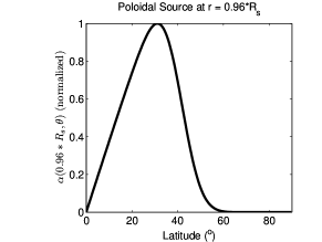
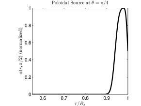
$(a)$ $(b)$

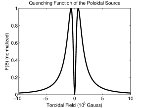
(c)

Figure 1: Latitudinal(a) and radial(b) dependence of the poloidal source as quantified by the dynamo $\alpha$-term. (c) Magnetic quenching of the poloidal source term.

where $\alpha_{0}$ sets the strength of the source term and we set it to the value in which our system starts having oscillating solutions. The parameters $\beta=40^{o}$ and $\gamma=10^{o}$ characterize the latitudes in which sunspots appear. On the other hand, $r_{al}=0.94R_{\odot}$, $d_{al}=0.04R_{\odot}$, $r_{ah}=R_{\odot}$ and $d_{ah}=0.01R_{\odot}$ characterize the radial extent of the region in which the poloidal field is deposited (see Figure 1-a and b). Besides radial and latitudinal dependence, we also introduce lower and upper operating thresholds on the poloidal source that is dependent on toroidal field amplitude – which is a more realistic representation of the physics involving magnetic buoyancy (as argued in Nandy & Choudhuri 2001; Nandy 2002; see also Charbonneau, St-Jean & Zacharias 2005). The presence of a lower threshold is in response to the fact that the plasma density inside weak flux tubes is not low enough (compared to the density of the surrounding plasma) to make them unstable to buoyancy (Caligari, Moreno-Insertis & Schussler 1995) and those that manage to rise have very long rising times (Fan, Fisher and De Luca 1993). On the other hand, if flux tubes are too strong they are not tilted enough when they reach the surface to contribute to poloidal field generation (D’Silva and Choudhuri 1993; Fan, Fisher and Deluca 1993). The dependence of the poloidal source on magnetic field is

$$F(B_{av})=\frac{K_{ae}}{1+\left(B_{av}/B_{h}\right)^{2}}\left(1-\frac{1}{1+\left(B_{av}/B_{l}\right)^{2}}\right),$$ (7)

where $K_{ae}=1/\max(F(B_{av}))$ is a normalization constant and $B_{h}=1.5\times 10^{5}G$ and $B_{l}=4\times 10^{4}G$ are the operating thresholds (see Figure 1-c).

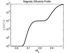
Figure 2: Radial dependence of the turbulent magnetic diffusivity.

Another ingredient of this model is a radially dependent magnetic diffusivity; in this work we use a double-step profile (see Figure 2) given by

$$\eta(r)=\eta_{bcd}+\frac{\eta_{cz}-\eta_{bcd}}{2}\left(1+\operatorname{erf}\left(\frac{r-r_{cz}}{d_{cz}}\right)\right)+\frac{\eta_{sg}-\eta_{cz}-\eta_{bcd}}{2}\left(1+\operatorname{erf}\left(\frac{r-r_{sg}}{d_{sg}},\right)\right)$$ (8)

where $\eta_{bcd}=10^{8}cm^{2}/s$ corresponds to the diffusivity at the bottom of the computational domain,$\eta_{cz}=10^{11}cm^{2}/s$ corresponds to the diffusivity in the convection zone, $\eta_{sg}=10^{13}cm^{2}/s$ corresponds to the supergranular diffusivity and $r_{cz}=0.73R_{\odot}$, $d_{cz}=0.03R_{\odot}$, $r_{sg}=0.95R_{\odot}$ and $d_{sg}=0.05R_{\odot}$ characterize the transitions from one value of diffusivity to the other. Although it is common these days to use these sort of profile, a point we note in passing is that the exact depth dependence of turbulent diffusivity within the SCZ is poorly, if at all, constrained. Besides the value of the supergranular diffusivity $\eta_{sg}$, which can be estimated by observations (Hathaway & Choudhary 2008), the others parameters are not necessarily well constrained.

Once all ingredients are defined(see Section 3 for the flow field), we solve the dynamo equations using a recently developed and novel numerical technique called exponential propagation (see Appendix). Our computational domain is defined in a $250\times 250$ grid comprising only one hemisphere. Since we run our simulations only in one hemisphere our latitudinal boundary conditions at the equator ($\theta=\pi/2$) are $\partial A/\partial\theta=0$ and $B=0$. Furthermore, since the equations we are solving are axisymmetric, both the potential vector and the toroidal field need to be zero ($A=0$ and $B=0$) at the pole ($\theta=0$), to avoid singularities in spherical coordinates. For the lower boundary condition ($r=0.55R_{\odot}$), we assume a perfectly conducting core, such that both the poloidal field and the toroidal field vanish there (i.e., $A,B=0$ at the lower boundary). For the upper boundary condition we assume that the magnetic field has only a radial component ($B=0$ and $\partial(rA)/\partial r=0$); this condition has been found necessary for stress balance between subsurface and coronal magnetic fields (for more details refer to van Ballegooijen and Mackay 2007). As initial conditions we set $A=0$ throughput our computational domain and $B\propto\sin(2\theta)*\sin(\pi*((r-0.55R_{\odot})/(R_{\odot}-0.55R_{\odot})))$. After a few cycles, all transients related to the initial conditions typically disappear and the dynamo settles into regular oscillatory solutions whose properties are determined by the parameters in the dynamo equations.

3 Constraining the Flow Fields

The last two ingredients of the dynamo model are the velocity fields (differential rotation and meridional circulation), which are the focus of this work. The differential rotation is probably the best constrained of all dynamo ingredients but the actual helioseismology data has never before been used directly in dynamo model, only an analytical fit to it. We discuss below how the actual rotation data can be used directly within dynamo models through the use of a weighting function to filter out the observational data in the region where it cannot be trusted. On the other hand, the meridional circulation is one of the most loosely constrained ingredients of the dynamo. Traditionally only the peak surface flow speed is used to constrain the analytical functions that are used to parameterize it, in conjunction with mass conservation. In this work we take advantage of the properties of such functions and make a fit to the helioseismic data on the meridional flow that constrains the location and extent of the polar downflow and equatorial upflow, as well as the radial dependence of the meridional flow near the surface – thereby taking steps towards better constrained flow profiles.

3.1 Differential Rotation

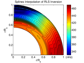
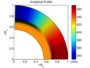
$(a)$	$(b)$
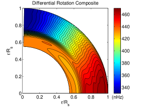
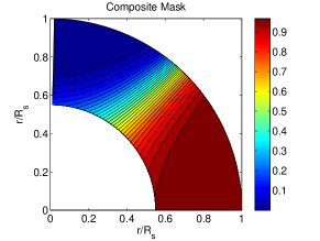
$(c)$	$(d)$

Figure 3: (a) Spline interpolation of the RLS inversion. (b) Analytical profile of Charbonneau et al. (1999). (c) Differential rotation composite used in our simulations. (d) weighting function used to create a composite between the RLS inversion and the analytical profile of Charbonneau et al. 1999. For all figures the red denotes the highest and blue the lowest value and the units are nHz with the exception of the weighting function.

As opposed to meridional circulation, there are helioseismic measurements of the differential rotation for most of the convective envelope which can be used directly in our simulations. Here we use data from the Global Oscillation Network Group (GONG) (courtesy Dr. Rachel Howe) obtained using the RLS inversion mapped onto a $51\times 51$ grid (see Figure 3-a). However, these observations cannot be trusted fully in the region within $0.3R_{\odot}$ of the rotation axis (specifically at high latitudes), because the inversion kernels have very little amplitude there. Below we outline a method to deal with this suspect data by creating a composite rotation profile that replaces these data at high latitudes with plausible synthetic data, that smoothly matches to the observations in the region of trust.

3.1.1 Adaptation of the Data to the Model

In the first step we use a splines interpolation in order to map the data to the resolution of our simulation (a grid of $250\times 250$ see Figure 3-a). The next step is to make a composite with the data and the analytical form of Charbonneau et al. (1999; see Figure 3-b). The analytical form is defined as:

$$\begin{array}[]{c}\Omega_{A}(r,\theta)=2\pi\left[\Omega_{c}+\frac{1}{2}\left(1-\texttt{erf}\left(\frac{r-r_{tc}}{w_{tc}}\right)\right)\left(\Omega_{e}-\Omega_{c}+(\Omega_{p}-\Omega_{e})\Omega_{S}(\theta)\right)\right]\\ \\ \Omega_{S}(\theta)=a\cos^{2}(\theta)+(1-a)\cos^{4}(\theta),\\ \end{array}$$ (9)

where $\Omega_{c}=432$ nHz is the rotation frequency of the core, $\Omega_{e}=470$ nHz is the rotation frequency of the equator, $\Omega_{p}=330$ nHz is the rotation frequency of the pole, $a=0.483$ is the strength of the $\cos^{2}(\theta)$ with respect to the $\cos^{4}(\theta)$ term, $r_{tc}=0.716$ the location of the tachocline and $w_{tc}=0.03$. We use the parameters defining the tachocline’s location and thickness as reported by Charbonneau et al. (1999) for a latitude of $60^{o}$. This is because they match the data better at high latitudes (which is the place where the data merges with the analytical profile) than those reported for the equator. This composite replaces the suspect data at high latitudes within $0.3R_{\odot}$ of the rotation axis with that of the analytic profile. However, it is important to note that at low latitudes, within the convection zone, the actual helioseismic data is utilized.

In order to make the composite we create a weighting function $m(r,\theta)$ with values between 0 and 1 for each grid-point defining how much information will come from the RLS data and how much from the analytical form (see Figure 3-d). We define the weighting function in the following way:

$$m(r,\theta)=1-\frac{1}{2}\left(1+\texttt{erf}\left(\frac{r^{2}\cos(2\theta)-r_{m}^{2}}{d_{m}^{2}}\right)\right),$$ (10)

where $r_{m}=0.5R_{\odot}$ is a parameter that controls the center of the transition and $d_{m}=0.6R_{\odot}$ controls the thickness. The resultant differential rotation profile, which can be seen in Figure 3-c, is then calculated using the following expression:

$$\Omega(r,\theta)=m(r,\theta)\Omega_{RLS}(r,\theta)+[1-m(r,\theta)]\Omega_{A}(r,\theta)$$ (11)

3.1.2 Differences Between the Analytical Profile and the Composite Data

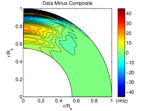
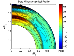
$(a)$	$(b)$

Figure 4: (a) Residual of subtracting the composite used in this work to the RLS inversion. (b) Residual of subtracting the analytical profile commonly used by the community to the RLS inversion. Red color corresponds to the hightest value and blue to the lowest. Graphs in units of nHz

It is instructive to compare the analytical and composite profiles with the actual helioseismology data. In Figure 4-a we present the residual error of subtracting the analytical profile of Charbonneau et al. (1999), with $r_{tc}=0.7$ and $w_{tc}=0.025$, from the RLS data. In Figure 4-b we present the residual error of subtracting our composite from the RLS data. As is expected, there is no difference between the composite and raw data at low latitude, but the residual increases as we approach the rotation axis – where the RLS data cannot be trusted. For the analytical profile, the residuals errors are more significant, even at low latitudes. This demonstrates the ability of our methodology to usefully integrate the helioseismic data for differential rotation.

3.2 Meridional Circulation

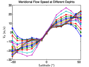
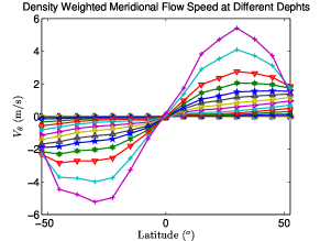
$(a)$ $(b)$

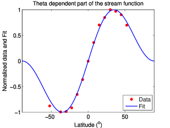
(c)

Figure 6: (a) Measured meridional flow as a function of latitude at different depths (Courtesy Dr. Irene González-Hernández), each combination of colors and markers corresponds to a different depth ranging from $0.97R_{\odot}$ to $R_{\odot}$. (b) Meridional flow after being weighted using solar density. If we sum all data points at each latitude we obtain the average velocity. (c) Normalized average velocity and analytical fit.

The meridional flow profile remains rather poorly constrained in the solar interior even though the available helioseismic data can be used to constrain the analytic flow profiles that are in use currently. Here we present ways to betters constrain this profile with helioseismic data. In order to do that, we use data from GONG (Courtesy Dr. Irene González-Hernández) obtained using the ring-diagrams technique. This data, which we can see in Figure 6-a, corresponds to a time average of the meridional flow between $2001$ and $2006$; and it comprises 19 values of $r$ from $R_{\odot}$ down to a depth of $0.97R_{\odot}$, and 15 different latitudes between $-52.5^{o}$ and $52.5^{o}$. It is important to note that our work relies heavily in the assumption that the meridional flow is adequately described by a stream function with separable variables. This is consistent with the assumption present implicitly in all work on axisymmetric solar dynamo models up to this date. Below we use this property of our stream function, along with weighted latitudinal and radial averages of the data, to completely constrain its latitudinal dependence, as well as the topmost ten percent of its radial dependence. As this data currently does not constrain the depth of penetration of the flow in the deep solar interior, we explore two different plausible penetration depths of the circulation. For reasons described later, we choose to perform simulations with two different peak meridional flow speeds, therefore exploring four plausible meridional flow profiles altogether.

3.2.1 Constraining the Latitudinal Dependence of the Meridional Flow

Meridional circulation has been typically implemented in these type of dynamo models by using a stream function in combination with mass conservation, i.e.:

$$\overrightarrow{\textbf{v}}_{p}\left(r,\theta\right)=\frac{1}{\rho(r)}\vec{\nabla}\times\left(\Psi(r,\theta)\widehat{\textbf{e}}_{\phi}\right).$$ (12)

The two stream functions that are commonly used were proposed by van Ballegooijen and Choudhuri (1988) and by Dikpati and Choudhuri (1995). They have in common the separability of variables and thus can be written in the following way:

$$\Psi(r,\theta)=v_{0}F(r)G(\theta),$$ (13)

where $v_{0}$ is a constant which controls the amplitude of the meridional flow.

Using such a stream function the components of the meridional flow become:

$$v_{r}(r,\theta)=v_{0}\frac{F(r)}{r\rho(r)}\frac{1}{\sin(\theta)}\frac{\partial}{\partial\theta}\left(\sin(\theta)G(\theta)\right),$$ (14)

$$v_{\theta}(r,\theta)=-v_{0}\frac{1}{r\rho(r)}\frac{\partial}{\partial r}(rF(r))G(\theta),$$ (15)

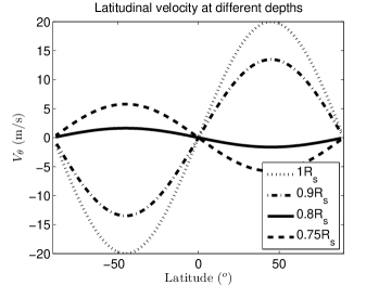
Figure 5: Latitudinal velocity as a function of $\theta$ used by van Ballegooijen and Choudhuri 1988 for different depths. Notice that the curves differ from each other only on their amplitude.

which can themselves be separated into the multiplication of exclusively radially and latitudinally dependent functions. This property allows us to constrain the entire latitudinal dependence of this family of functions by using the available helioseismology data for $v_{\theta}$ at the surface. This can be done because the latitudinal dependence of $v_{\theta}$ is exactly the same as that of the stream function and only the amplitude of this functional form changes with depth, see for example Figure 5 for the latitudinal velocity at different depths used by van Ballegooijen and Choudhuri (1988). In this work we assume a latitudinal dependence like the one they used, i.e.,

$$G(\theta)=\sin^{(q+1)}(\theta)\cos(\theta).$$ (16)

In order to estimate the parameter $q$ we first take a density weighted average of the helioseismic data using the values for solar density from the Solar Model S (Christensen-Dalsgaard et al. 1996), such that

$$\bar{v}_{\theta}(\theta_{j})=\frac{\sum_{i}v_{\theta}(r_{i},\theta_{j})\rho(r_{i})}{\sum_{i}\rho(r_{i})}.$$ (17)

In Figure 6-b we plot the meridional flow at different depths weighted by density, which we add for each latitude in order to find the average. We then use this average to make a least squares fit to the analytical expression (eq 16), which we can see in Figure 6-c. We find that a value of $q=1$ fits the data best. This therefore constrains the latitudinal ($\theta$) dependence of the flow profile.

3.2.2 Constraining the Radial Dependence of the Meridional Flow

As opposed to the latitudinal dependence, the radial dependence of the meridional flow is less constrained since there is no data below $0.97R_{\odot}$. However, at least some of the parameters can be constrained: We start with the solar density, for which we perform a least squares fit to the Solar Model S using the following expression:

$$\rho(r)\sim\left(\frac{R_{\odot}}{r}-\gamma\right)^{m}$$ (18)

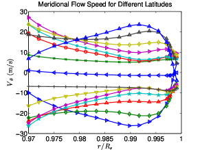
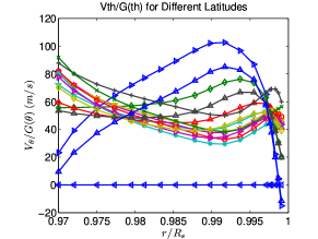
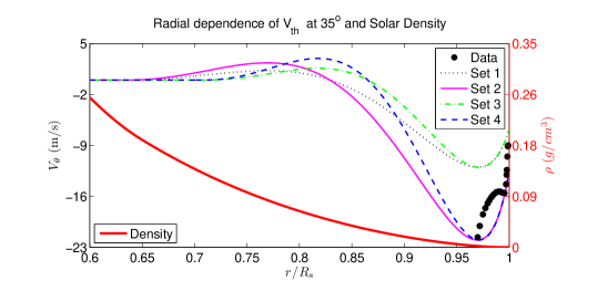
[h] $(a)$ $(b)$ (c)

Figure 7: (a) Measured meridional flow as a function of radius at different latitudes (Courtesy Dr. Irene González-Hernández), each combination of colors and markers corresponds to a different latitude varying from $-52.5$ to $52.5$. (b) Meridional flow after removing the latitudinal dependence, i. e. $v_{\theta}/G(\theta)$. The horizontal line with zero latitudinal velocity corresponds to the Equator. (c) Radial dependence of the latitudinally averaged meridional flow for our helioseismic data is depicted as large black dots. Other curves correspond to the radial dependence of the meridional flow profiles used in our simulations and solar density: Set 1 (black dotted) $R_{p}=0.64R_{\odot}$, $v_{o}=12m/s$; Set 2 (magenta solid) $R_{p}=0.64R_{\odot}$, $v_{o}=22m/s$; Set 3 (green dash-dot) $R_{p}=0.71R_{\odot}$, $v_{o}=12m/s$ and Set 4 (blue dashed line) $R_{p}=0.71R_{\odot}$, $v_{o}=22m/s$. The solar density taken from the solar Model S (Christensen-Dalsgaard et al. 1996) is depicted as a solid red line. The left-vertical axis is in units of velocity and the right-vertical is in units of density.

we find that values of $\gamma=0.9665$ and $m=1.911$ fit the model best (see Figure 7-c).

In the second step we constrain the radial dependence of the stream function. We begin with the function

$$F(r)=\frac{1}{r}(r-R_{p})(r-R_{\odot})\sin\left(\pi\frac{r-R_{p}}{R_{1}-R_{p}}\right)^{a},$$ (19)

where $R_{\odot}$ corresponds to the solar radius, $R_{p}$ to the maximum penetration depth of the meridional flow and $a$ and $R_{1}$ control the location in radius of the poleward peak and the value of the meridional flow at the surface. In order to constrain them we use the helioseismic data again, but this time we use the radial dependence (see Figure 7-a). We first remove the latitudinal dependence, which we do by dividing the data of each latitude by $G(\theta)$ using the value of $q=1$ found in the previous section. In Figure 7-b we plot the flow data after removing the latitudinal dependence, note that there is no longer any sign difference between the two hemispheres. The next step is to generate the latitudinal average which we can see as black dots in Figure 7-c. It is evident from looking at the radial dependence of the meridional flow that the velocity increases with depth for most latitudes, and that the point of maximum velocity is not within the depth up to which the data extends. Since the exact radial dependence of the data is too complex for our functional form to grasp, the features we concentrate on reproducing are the presence of a maximum inside the convection zone, as well as the amplitude of the flow at the near surface-layers. The logic here is to use the fewest possible parameters and a simple, physically transparent profile that does a reasonable job of matching the data. In view of the lack of better constraints, we assume here that the peak of the return flow is at $0.97R_{\odot}$ (which is the depth at which the current helioseismic data has it’s peak).

Following the procedures and steps above we construct profiles to fit the depth-dependence pointed out in the available helioseismic data; however, this does not constrain how far the meridional flow can penetrate and therefore we try two different penetration depths, one shallow $0.71R_{\odot}$ (i.e., barely beneath the base of the SCZ) and one deep $R_{p}=0.64R_{\odot}$ (into the radiative interior) – both of which match the latitudinal and radial constraints as deduced from the near-surface helioseismic data. Note that observed light element abundance ratios limit the depth of penetration of the circulation to about $R_{p}=0.62R_{\odot}$ (Charbonneau 2007). Now we know that the meridional flow speed is highly variable, with fluctuations that can be quite significant and the measured flow speed can change depending on the phase of the solar cycle (Hathaway 1996; Gizon & Rempel 2008). The magnetic fields are also expected to feed back on the flow (Rempel 2006). Taken together these considerations point out that the effective meridional flow speed to be used in dynamo simulations could be less than that implied from the González-Hernández et al. data, a possibility that is borne out by the work of Braun & Fan (1998) and Gizon & Rempel (2008), who find much lower peak flow speeds in the range $12$–$15$ m/s. Keeping this in mind, we use the same latitudinal and radial constraint as deduced earlier, but consider in our simulations two additional profiles with peak flow speeds of $12$ m/s with deep and shallow penetrations. Therefore, in total we explore four plausible meridional flow profiles in our dynamo simulations (see Figure 7-c and Table 1 for an overview), the results of which are presented in the next section.

	$v_{o}$	$R_{p}$	$a$	$R_{1}$
Set 1	$12$ m/s	$0.64R_{\odot}$	$1.795$	$1.027R_{\odot}$
Set 2	$22$ m/s
Set 3	$12$ m/s	$0.71R_{\odot}$	$2.03$	$1.03R_{\odot}$
Set 4	$22$ m/s

Table 1: Sets of parameters characterizing the different meridional flow profiles used in our dynamo simulations. $v_{o}$ corresponds to the meridional flow peak speed, $R_{p}$ the maximum penetration of the flow, and $a$ and $R_{1}$ are parameters that control the location of the poleward flow as well as the surface speed.

4 Dynamo Simulation: Results and Discussions

4.1 Analytic vs. Helioseismic Composite Differential Rotation

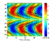
	$R_{p}=0.64R_{\odot}$
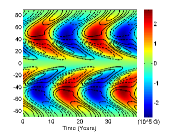
	$v_{o}=12$m/s
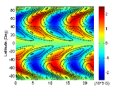
	$R_{p}=0.64R_{\odot}$
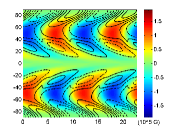
	$v_{o}=22$m/s
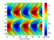
	$R_{p}=0.71R_{\odot}$
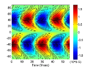
	$v_{o}=12$m/s
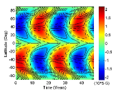
	$R_{p}=0.71R_{\odot}$
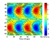
Composite DR	$v_{o}=22$m/s	Analytical DR

Figure 8: Butterfly diagram of the toroidal field at the bottom of the convection zone (color) with radial field at the surface (contours) superimposed on it. Each row corresponds to one of the different meridional circulation sets. The left column corresponds to runs using the helioseismic composite and the right one to runs using the analytical profile.

We first compare dynamo solutions found using the helioseismology composite of the differential rotation (Section 3.1.1) and the analytical profile of Charbonneau et al. (1999). In doing so, we perform simulations with a model as described in Section $2$ (see also numerical methods in the Appendix) and generate field evolution maps for the toroidal and poloidal fields. From the simulated butterfly diagrams for the evolution of the toroidal field at the base of the SCZ and the surface-radial field evolution (Figure 8), we find that large-scale features of the simulated solar cycle are generally similar across the two different rotation profiles (even with different meridional flow penetration depths and speeds), specially for the shallowest penetration (sets $3$ and $4$ with $R_{p}=0.71R_{\odot}$).

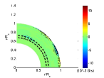
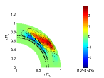
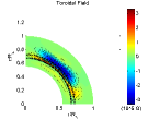
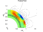
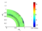
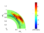
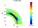
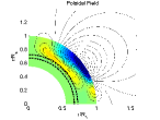
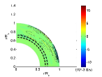
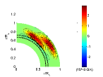
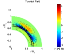
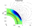
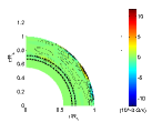
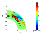
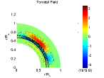
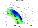
Figure 10: Snapshots of the shear source terms and the magnetic field over half a dynamo cycle (a sunspot cycle). Each row is advanced by an eight of the dynamo cycle (a quarter of the sunspot cycle) i.e., from top to bottom $t=0,\tau/8,\tau/4$ and $3\tau/8$. The solution corresponds to the composite differential rotation and meridional flow Set 1 (deepest penetration with a peak flow of 12 m/s)

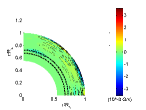
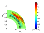
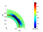
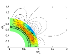
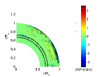
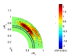
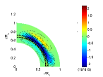
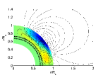
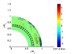
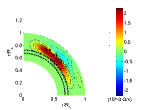
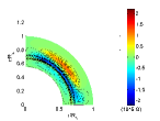
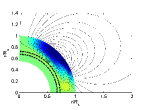
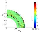
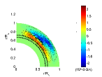
Figure 11: Snapshots of the shear source terms and the magnetic field over half a dynamo cycle (a sunspot cycle). Each row is advanced by an eight of the dynamo cycle (a quarter of the sunspot cycle) i.e., from top to bottom $t=0,\tau/8,\tau/4$ and $3\tau/8$. The solution corresponds to the composite differential rotation and meridional flow Set 4 (shallowest penetration with a peak flow of 22 m/s)

In order to understand this similarity, it is useful to look at Figures 10 and 11 corresponding to simulations using the composite differential rotation, and the meridional flow sets $1$ ($R_{p}=0.64R_{\odot}$, $v_{o}=12m/s$) and $4$ ($R_{p}=0.71R_{\odot}$, $v_{o}=22m/s$). The first two columns, from left to right of both figures show the evolution of the shear sources $(\textbf{B}_{r}\cdot\nabla_{r}\Omega)$ and $(\textbf{B}_{\theta}\cdot\nabla_{\theta}\Omega)$ – which contribute to toroidal field generation by stretching of the poloidal field. It is evident that the location and strength of these sources is different – the radial shear source is mainly present near the surface whereas the latitudinal shear is spread throughout the convection zone. It can also be seen that the radial shear source is roughly five times stronger than the latitudinal. However, if attention is paid to the evolution of the toroidal field (third column from the right in both figures), it is clear that this radial shear term has no significant impact on the structure and magnitude of the toroidal field (a similar result was found by Dikpati et al. 2002). The reason is that the upper boundary condition ($B=0$ at $r=R_{\odot}$), in combination with the high turbulent diffusivity (and thus short diffusive time scale) there, imposes itself very quickly on the toroidal field generated by the radial shear – washing it out. This greatly reduces the relative role of the surface shear as a source of toroidal magnetic field, effectively making the surface dynamics very similar across simulations using the analytical rotation profile (without any surface shear) or the composite helioseismic profile.

Once the surface layers are ruled out as important sources of toroidal field generation we are faced with the fact that the strongest source of toroidal field is the latitudinal shear inside the convection zone (and not the tachocline radial shear), as is evident in Figures 10 and 11. This goes against the commonly held perception that the tachocline is where most of the toroidal field is produced. However, the importance of the latitudinal shear term in the SCZ is clearly demonstrated here where we have plotted the shear source terms, which is not normally done by dynamo modelers.

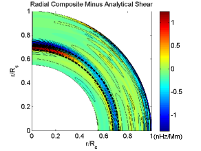
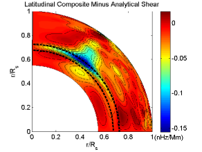
[h] $(a)$ $(b)$

Figure 9: (a) Residual after subtracting the radial shear of the analytical profile commonly used by the community from the radial shear of our composite data. (b) Residual of subtracting the latitudinal shear of the analytical profile commonly used by the community from the latitudinal shear of our composite data.

The establishment of the SCZ as an importance source region of toroidal field is of relevance when regarding the similarity of the solutions obtained using the composite data and the analytical profile. This is because the region where the shear of the analytical profile and the helioseismic composite data differ most (both for radial and latitudinal shear) is in the tachocline. This is evident in Figure 9 where we plot the residual of subtracting the radial and latitudinal shear of the analytical profile from the shear of the composite data. The similarity between solutions is specially important for shallow meridional flow profiles with low penetration – which does not transport any poloidal field into the deeper tachocline, thereby further diminishing the role of the tachocline shear.

4.2 Shallow versus Deep Penetration of the Meridional Flow

In the second part of our work we compare dynamo solutions obtained for each of the four different meridional flow profiles with two different penetration depth and with two different peak flow speeds. First, from Figure 8 it is evident that the shape of the solutions changes with varying penetration depth; this is caused by the increasing role of the tachocline shear in generation and storage of the toroidal field as the penetration depth of the meridional flow increases. This is apparent when one compares Figure 10 (deep penetration) to Figure 11 (shallow penetration). If we look at the inductive shear sources it is evident that for the shallowest penetration no field is being generated inside the tachocline. In the poloidal field plots (right column) we see that no poloidal field is advected into the tachocline region for the shallowest penetration, but some is advected for the deepest.

Second we compare the periods of our solutions in Table 2: We find that most solutions have a sunspot cycle (i.e., half-dynamo cycle) period that is comparable to that of the Sun, with the exception of the fast flow with deep penetration and the slow flow with shallow penetration, which have respectively a comparatively smaller and larger period. As the meridional flow is buried deeper, one expects the length of the advective circuit to increase, thereby resulting in larger dynamo periods. However, it is evident that as we increase the penetration, the period decreases – even if the length of the flow loop that supposedly transports magnetic flux increases; this is counterintuitive but has a simple explanation. Our simulations and exhaustive analysis points out that it is not how deep the flow penetrates that governs the cycle period, but it is the magnitude of the meridional counterflow right at the base of the SCZ ($R_{p}=0.713R_{\odot}$) that is most relevant. This is because most of the poloidal field creation at near-surface layers is coupled to buoyant eruptions of toroidal field from this layer of equatorward migrating toroidal field belt at the base of the SCZ (see third columns in Figures 10 and 11) and it is the flow speed at this region that governs the dynamo period. In Figure 7 it is clear that the speed of the counterflow in this convection zone–radiative interior interface increases as the flow becomes more penetrating (a consequence of the constraints set by mass conservation and the fits to the near-surface helioseismic data), thereby reducing the dynamo period.

Overall, an evaluation of the butterfly diagram (Figure 8), points out that the toroidal field belt extends to lower latitudes (where sunspots are observed) for deeper penetrating meridional flow, although there is a polar branch as well. For the shallow flow, we find that the toroidal field belt is concentrated around mid-latitudes with almost symmetrical polar and equatorial branches – a signature of the convection zone latitudinal shear producing most of the toroidal field (as in the interface dynamo models, see, e.g., Parker 1993 and Charbonneau & MacGregor 1997).

	$R_{p}$	$v_{o}$	$\tau$ - HS data (yrs)	$\tau$ - Analytical (yrs)
Set 1	$0.64R_{\odot}$	$12$ m/s	$9.67$	$10.00$
Set 2		$22$ m/s	$5.63$	$5.67$
Set 3	$0.71R_{\odot}$	$12$ m/s	$14.67$	$14.02$
Set 4		$22$ m/s	$11.85$	$12.85$

Table 2: Simulated sunspot cycle period for the different sets of meridional flow parameters. $R_{p}$ corresponds to the maximum penetration depth of the meridional flow, $v_{o}$ to the peak speed in the poleward flow and $\tau$ is the period of the solutions in units of years. For the rest of the parameters in each set please refer to Table 1

4.3 Dependence of the solutions on changes in the turbulent diffusivity profile

Although a detailed exploration of the turbulent diffusivity parameter space is outside the scope of this work, we study two special cases in which we vary a single parameter while leaving the rest fixed.

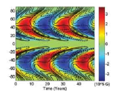
	$R_{p}=0.64R_{\odot}$
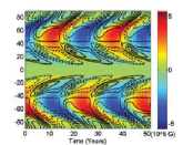
	$v_{o}=12$m/s
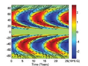
	$R_{p}=0.64R_{\odot}$
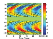
	$v_{o}=22$m/s
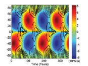
	$R_{p}=0.71R_{\odot}$
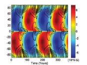
	$v_{o}=12$m/s
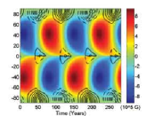
	$R_{p}=0.71R_{\odot}$
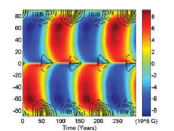
Composite DR	$v_{o}=22$m/s	Analytical DR

Figure 12: Butterfly diagram of the torodial field at the bottom of the convection zone (Color) with radial field at the surface (Contours) superimposed on it when using a low diffusivity in the convection zone ($\eta_{cz}=10^{10}cm^{2}/s$). Each row corresponds to one of the different meridional circulation sets. The left column corresponds to runs using the helioseismology composite and the right one to runs using the analytical profile.

For the first case we lower the diffusivity in the convection zone, $\eta_{cz}$, from $10^{11}cm^{2}/s$ to $10^{10}cm^{2}/s$. As can be seen in Figure 12, this introduces two important changes in the dynamo solutions: The first one is an overall increase in magnetic field magnitude due to the reduction in diffusive decay while keeping the strength of the field sources constant. The second is a drastic increase in the dynamo period (which can be seen tabulated in Table 3) for the solutions that use a meridional flow with a penetration of $R_{p}=0.71R_{\odot}$. The reason behind such a change resides in the nature of the transport processes at the bottom of the convection zone, which are a combination of both advection and diffusion. In the case of flow profiles with deep penetration the velocity at the bottom is high enough for downward advection to transport flux into the tachocline. On the other hand, in the case of low penetration, the last bit of downward transport into the tachocline is done by diffusive transport and thus dominated by diffusive timescales. Because of this, by decreasing turbulent diffusivity by an order of magnitude, we drastically increase the period of the solutions.

	$R_{p}$	$v_{o}$	$\tau$ - HS data (yrs)	$\tau$ - Analytical (yrs)
Set 1	$0.64R_{\odot}$	$12$ m/s	$12.46$	$12.86$
Set 2		$22$ m/s	$6.47$	$6.55$
Set 3	$0.71R_{\odot}$	$12$ m/s	$87.78$	$90.92$
Set 4		$22$ m/s	$70.48$	$74.41$

Table 3: Simulated sunspot cycle period for the different sets of meridional flow parameters when using a low diffusivity in the convection zone ($\eta_{cz}=10^{10}cm^{2}/s$). $R_{p}$ corresponds to the maximum penetration depth of the meridional flow, $v_{o}$ to the peak speed in the poleward flow and $\tau$ is the period of the solutions in units of years.

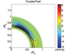
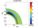
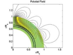
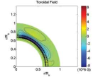
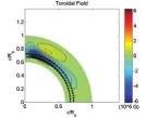
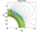
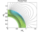
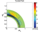
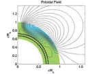
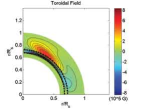
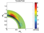
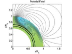
Figure 13: Snapshots of the magnetic field over half a dynamo cycle (a sunspot cycle) when using a low super-granular diffusivity ($\eta_{cz}=10^{11}cm^{2}/s$). Each row is advanced by an eight of the dynamo cycle (a quarter of the sunspot cycle) i.e., from top to bottom $t=0,\tau/8,\tau/4$ and $3\tau/8$. The solutions correspond to the meridional flow Set 2 (deepest penetration with a peak flow of 12 m/s) and analytic differential rotation (left) and composite data (right)

In the second parameter space experiment, we lower the super-granular diffusivity $\eta_{sg}$ from $10^{13}cm^{2}/s$ to $10^{11}cm^{2}/s$. This was done to study the impact of the surface radial shear under low diffusivity conditions. However, as can be seen in Figure 13, there is very little difference between the two solutions. This means that even after reducing the super-granular diffusivity by two orders of magnitude, the radial shear has very little impact on the solutions and the upper boundary conditions still play an important role in limiting the relative contribution from the near-surface shear layer.

5 Conclusions

In summary, we have presented here methods which can be used to better integrate helioseismic data into kinematic dynamo models. In particular, we have demonstrated that using a composite between helioseismic data and an analytical profile for the differential rotation, we can directly use the helioseismic rotation data in the region of trust and substitute the suspect data by smoothly matching it to the analytical profile where the data is noisy. This paves the way for including the helioseismically inferred rotation profile directly in dynamo simulations. We have also shown how mathematical properties of the commonly used analytic stream functions describing the meridional flow can be fit to the available near-surface helioseismic data to entirely constrain the latitudinal dependence of the meridional flow, as well as weakly constrain the radial (depth) dependence.

In our simulations, comparing the helioseismic data for the differential rotation with the analytical profile of Charbonneau et al. (1999), with four plausible meridional flow profiles, we find that there is little difference between the solutions using the helioseismic composite and the analytical differential rotation profile – specially for shallow penetrations of the meridional flow and even at reduced super-granular diffusivity. This is because the impact of the surface radial shear, which is present in the helioseismic composite but not the analytic profile, is greatly reduced by the proximity of the upper boundary conditions. Also, for the shallow circulation, the toroidal field generation occurs in a region located above the tachocline with mainly latitudinal shear, where the difference between the composite data and the analytical profile is not significant.

The main result from this comparative analysis is that the latitudinal shear in the rotation is the most dominant source of toroidal field generation in these type of models that are characterized by high diffusivity at near surface layers, but lower diffusivity within the bulk of the SCZ – specially near the base where most of the toroidal field is being created. Since this latitudinal shear exists throughout the convection zone, an interesting question is whether toroidal fields can be stored there long enough to be amplified to high values by the shear in the rotation, without being removed by magnetic buoyancy. If this were to be the case, i.e., the latitudinal shear is indeed confirmed to be the dominant source of toroidal field induction, we anticipate then that downward flux pumping (Tobias et al. 2001; see also Guerrero & de Gouveia Dal Pino 2008) – which tends to act against buoyant removal of flux, may have an important role to play in this context. This could also call into question the widely held view that the solar tachocline is where most of the toroidal field is created and stored (see Brandenburg 2005 for arguments favoring a more distributed dynamo action throughout the SCZ).

Our attempts to integrate helioseismic meridional flow data into dynamo models and related simulations have uncovered points that are both encouraging and discouraging.

On the discouraging side, we find that the currently available observational data are inadequate to constrain the nature and exact profile of the deep meridional flow, especially the return flow. Neither do the simulation results and their comparison with observed features of the solar cycle clearly support or rule out any possibility. A recent analysis on light-element depletion due to transport by meridional circulation indicates that solar light-element abundance observations restrict the penetration to $0.62R_{\odot}$ (Charbonneau 2007); however this analysis does not necessarily suggest that the flow does penetrate that deep. Also vexing is the fact that different inversions, involving different helioseismic techniques such as ring-diagram or time-distance analysis recovers different profiles and widely varying peak meridional flow speeds (Giles et al. 1997; Braun & Fan 1998; González-Hernández et al. 2006; Gizon & Rempel 2008). In our analysis, we chose to use the González-Hernández et al. data because at present, this provides the (relatively) deepest full inversion of the flow within the SCZ. Chou and Ladenkov (2005) reported time-distance diagrams reaching a depth of $0.79R_{\odot}$ but have not yet reported a full inversion that could be used on our simulations.

We point out that there is an important consequence of the presence of the flow speed maximum inside the convection zone – which is related to mass conservation: If the maximum poleward flow speed is found to be deeper inside the convection zone this would result in a stronger mass flux poleward, which needs to be balanced by a deeper counterflow subject to mass conservation; the density of the plasma increases rapidly as one goes deeper; e.g., the density at $0.97R_{\odot}$ is ten thousand times larger than at the surface. Although that is not achieved currently, our extensive efforts to fit the data point out that stronger constraints on the return flow may be achieved even with data that does not necessarily go down to where this return flow is located, a fact that may be usefully utilized when better depth-dependent helioseismic data on meridional circulation becomes available.

Although the depth of penetration of the circulation is an important constraint on the flow itself, our results indicate that the period of of the dynamo cycle does not in fact depend on this depth. Rather, our simulations point out that the period of the dynamo cycle is more sensitive to changes on the speed of the counterflow than changes anywhere else in the transport circuit, as this is where the dynamo loop originates. An accurate determination of the average meridional flow speed over this loop closing at the SCZ base is very important in the context of the field transport timescales. As shown by the analysis of Yeates, Nandy & Mackay (2008), the relative timescales of circulation and turbulent diffusion determines whether the dynamo operates in the advection or diffusion dominated regime – two regimes which have profoundly different flux transport dynamics and cycle memory (the latter may lead to predictability of future cycle amplitudes). Getting a firm handle on the average meridional flow speed is therefore very important and that is not currently achieved from the diverging helioseismic inversion results on the meridional flow.

This suggests that a concerted effort using different helioseismic techniques on data for the meridional flow over at least a complete solar cycle (over the same period of time) may be necessary to generate a more coherent picture of the observational constraint on this flow profile. It’s important to note that even though we used time averaged data, nothing prevents one from using the same methods to assimilate time dependent helioseismic data at different phases of the solar circle, allowing us to study the impact of time varying velocity flows on solar cycle properties and their predictability.

On the encouraging side, our dynamo simulations show that it is relatively straightforward to use the available helioseismic data on the differential rotation (on which there is more consensus and agreement across various groups) within dynamo models. Also encouraging is the fact that the type of solar dynamo model presented here is able to handle the real helioseismic differential rotation profile and generate solar-like solutions. Moreover, as evident from our simulations, this dynamo model also generates plausible solar-like solutions over a wide range of meridional flow profiles, both deep and shallow, and with fast and slow peak flow speeds. This certainly bodes well for assimilating helioseismic data to construct better constrained solar dynamo models – building upon the techniques outlined here.

6 Acknowledgements

We are grateful to Irene González-Hernández and Rachel Howe at the National Solar Observatory for providing us with helioseismic data and useful counsel regarding it’s use. We also thank Jørgen Christensen-Dalsgaard of the Danish AsteroSeismology Center for data and discussions related to the solar Model S. Finally, we want to thank Paul Charbonneau and an anonymous referee for useful comments and recommendations. The simulations presented here were performed at the computing facilities of the Harvard Smithsonian Center for Astrophysics and this research was funded by NASA Living With a Star Grant NNX08AW53G to the Smithsonian Astrophysical Observatory.

Appendix A Numerical methods

In order to use exponential propagation, we transform our system of Partial Differential Equations(PDEs) in to a system of coupled Ordinary Differential Equations(ODEs) by discretizing the spatial operators using the following finite difference operators:

For advective terms $\left(\frac{\partial A}{\partial t}=-v\frac{\partial A}{\partial x}+\chi(x)\right)$, where $v$ is the velocity, we use a third order upwind scheme:

$$v\frac{\partial A}{\partial x}=\left\{\begin{array}[]{cc}\frac{v}{6\triangle x}(-2A_{i-1}-3A_{i}+6A_{i+1}-A_{i+2})&\mbox{if $v<0$}\\ \frac{v}{6\triangle x}(2A_{i+1}+3A_{i}-6A_{i-1}+A_{i-2})&\mbox{if $v\geq 0$}\\ \end{array}\right.+\mathcal{O}(\triangle x^{3})$$ (A1)

For diffusive terms $\left(\frac{\partial A}{\partial t}=\eta\frac{\partial^{2}A}{\partial x^{2}}+\chi(x)\right)$, where $\eta$ is the diffusion coefficient, we use a second order space centered scheme:

$$\eta\frac{\partial^{2}A}{\partial x^{2}}=\frac{\eta}{(\triangle x)^{2}}(A_{i-1}-2A_{i}+A_{i+1})+\mathcal{O}(\triangle x^{2})$$ (A2)

For other first derivative terms $\left(\frac{\partial A}{\partial t}=\frac{\partial B}{\partial x}+\chi(x)\right)$ we use a second order space centered scheme:

$$\frac{\partial B}{\partial x}=\frac{1}{2\triangle x}(A_{i-1}-A_{i+1})+\mathcal{O}(\triangle x^{2})$$ (A3)

Here, $\chi(x)$ corresponds to all the additional terms a PDE might have on the righthand side besides the term under discussion and $A_{i}=A(x_{0}+i\triangle x),i=1,2,...,N_{x}$ is our variable evaluated in a uniform grid of $N_{x}$ elements separated by a distance $\triangle x$.

A.1 Exponential Propagation

After discretization and inclusion of the boundary conditions we are left with an initial value problem of ordinary differential equations:

$$\frac{\partial\textbf{U}(t)}{\partial t} = F(\textbf{U}(t))$$ (A4)

$$\textbf{U}(t_{0}) = \textbf{U}_{0}$$ (A5)

where U is the solution vector in $\mathbb{R}^{N}$. Provided that the Jacobian $\partial F(\textbf{U}(t))$ exists and is continuous in the interval $[t_{0},t_{0}+\Delta t]$, we can linearize $F(\textbf{U}(t_{0}+\Delta t))$ around the initial state to obtain

$$\frac{\partial\textbf{U}(t)}{\partial t}=F(\textbf{U}_{0})+\partial F(\textbf{U}_{0})(\textbf{U}(t_{0}+\Delta t)-\textbf{U}_{0})+R(\textbf{U}(t_{0}+\Delta t))$$ (A6)

where $R(\textbf{U}(t_{0}+\Delta t)$ are the residual high order terms. The solution to this equation can be written as

$$\textbf{U}(t_{0}+\Delta t)=\textbf{U}_{0}+\frac{e^{A\Delta t}-I}{A}+\mathcal{O}(\Delta t^{2})$$ (A7)

where $A=\partial F(\textbf{U}_{0})$. Neglecting higher order terms leaves us with a scheme that is second order accurate in time and is an exact solution of the linear case. However there is a way of increasing the time accuracy of this method by following a generalization of Runge-Kutta methods for non-linear time-advancement operators proposed by Rosenbrock (1963). The combination of exponential propagation with Runge-Kutta methods was first proposed by Hochbruck and Lubich (1997) and then generalized by Hochbruck, Lubich and Selhofer (1998). In this work we use a fourth order algorithm which goes to the following intermediary steps to advance the solution vector between timesteps ($\textbf{U}^{n})\rightarrow\textbf{U}^{n+1})$):

$$k_{1} = \Phi\left(\frac{1}{2}\Delta tA\right)F(\textbf{U}^{n})$$

$$k_{2} = \Phi\left(\Delta tA\right)F(\textbf{U}^{n})$$

$$w_{3} = \frac{3}{8}(k_{1}+k_{2})$$

$$u_{3} = \textbf{U}^{n}+\Delta tw_{3}$$

$$d_{3} = F(u_{3})-F(\textbf{U}^{n})-\Delta tAw_{3}$$

$$k_{3} = \Phi\left(\frac{1}{2}\Delta tA\right)d_{3}$$

$$\textbf{U}^{n+1} = \textbf{U}^{n}+\Delta t\left(k_{2}+\frac{16}{27}k_{3}\right)$$

$$A=F(\textbf{U}^{n}) \Phi\left(\Delta tA\right)=\frac{e^{A\Delta t}-I}{A}$$ ,

A.2 Krylov Approximation to the Exponential Operator

Without any further approximation, this method is very expensive computationally due to the need of continuously evaluating the matrix exponential. However, it is possible to make a good approximation by projecting the operator into a finite dimensional Krylov subspace

$$S_{Kr}=\operatorname{span}\{\textbf{U}_{0},A\textbf{U}_{0},A^{2}\textbf{U}_{0},...,A^{m-1}\textbf{U}_{0}\}.$$ (A8)

In order to do this we first compute an orthonormal basis for this subspace using the Arnoldi algorithm (Arnoldi 1951):

1. $v_{1}=\textbf{U}_{0}/|\textbf{U}_{0}|^{2}$

2. For $j=1,...,m$ do

   • for $i=1,...,i$ compute $h_{i,j}=v_{i}^{T}*Av_{j}$

   • calculate $w=Av_{j}-\displaystyle\sum_{i=0}^{j}h_{i,j}v_{i}$

   • evaluate $h_{(}j+1,j)=|w|^{2}$

   • if $h_{j+1,j}<\epsilon$ stop, else compute the next basis vector $v_{j+1}=w/h_{j+1,j}$

where $\epsilon$ is the parameter that sets the error tolerance in this approximation. Once we have finished computing the algorithm, we have the relationship

$$AV_{m}\approx V_{m}H,$$ (A9)

where $V_{m}=[v_{1},...,v_{m}]$ and H is a matrix whose elements are $h_{i,j}=v_{i}^{T}*Av_{j}$. The validity of this approximation depends on the dimension of the Krylov subspace but numerical experiments have found that 15-30 Krylov vectors are usually enough (see Hochbruck and Lubich 1997; Tokman 2001). Since $\{v_{1},...,v_{m}\}$ is an orthonormal basis of the Krylov subspace $S_{Kr}$ then $V_{m}^{T}V_{M}$ is a $m\times m$ identity matrix and $V_{m}V_{m}^{T}$ is a projector from $\mathbb{R}^{N}$ onto $S_{Kr}$. Using this projector we can find an approximation to any matrix vector multiplication by projecting them onto the Krylov subspace by calculating $Ab\approx V_{m}V_{m}^{T}AV_{m}V_{m}^{T}b$. After using Equation A9 this becomes

$$Ab\approx V_{m}HV_{m}^{T}b.$$ (A10)

In fact we can approximate the action of any operator $\Phi(A)$, that can be expanded on a Taylor series, on the vector $\textbf{U}_{0}$ using the Krylov subspace projection:

$$\Phi(A)\textbf{U}_{0}\approx V_{m}\Phi(H)V_{m}^{T}\textbf{U}_{0}=|\textbf{U}_{0}|^{2}V_{m}\Phi(H)e_{1}$$ (A11)

where $e_{1}=$ $[1$ $0$ … $0]$ and we used $v_{1}=\textbf{U}_{0}/|\textbf{U}_{0}|^{2}$ and $V_{m}^{T}v_{1}=e_{1}$. As we can see in Equation A11, the use of the Krylov approximation effectively reduces the size of the matrix operator; this makes the use of the exponential operator relatively inexpensive computationally.

These two algorithms, in combination with a robust error control and an adaptative time-step mechanism strategy, form the core of the SD-Exp4 integrator (for more details see Hochbruck and Lubich 1997; Hochbruck, Lubich and Selhofer 1998 and Tokman 2001).

In order to verify the performance standards of the SD-Exp4 code we ran case C’ of the dynamo benchmark by Jouve et al. (2008). This case is similar in nature to the simulations done in this work with the following differences:

• The meridional flow profile has different radial and latitudinal dependence.

• The poloidal source term has no quenching term and a different radial and latitudinal dependence.

• The turbulent diffusivity profile consists of only one step and reaches a peak value of $10^{11}$ $cm^{2}/s$.

• The analytic differential rotation has no $cos^{4}(\theta)$ dependence and uses a thinner tachocline.

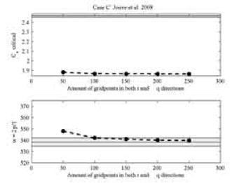
Figure 14: Simulation results (dots) of running case C’ of the dynamo benchmark by Jouve et al. (2008). The top figure shows how the minimum value of $C_{\alpha}=\alpha_{0}R_{\odot}/\eta_{cz}$ for which the dynamo has stable oscillations depends on resolution. The bottom figure shows how $\omega=2\pi R_{\odot}^{2}/(T\eta_{cz})$ depends on resolution. In order to make the plot comparable to the benchmark, we include the mean value found by the different codes and a shaded area corresponding to one standard deviation around this mean. This run was made using the same meridional flow and poloidal source profiles as in the benchmark study (for details see Jouve et al. 2008).

In order to compare the performance of the different codes in the benchmark study, two quantities are used: $C^{crit}_{s}=\alpha^{crit}_{0}R_{\odot}/\eta_{cz}$ which quantifies the minimum strength of the source-relative-to-dissipation that yields stable oscillations and $\omega=2\pi R_{\odot}^{2}/(T\eta_{cz})$ which quantifies the frequency of the magnetic cycle relative to the diffusion timescale. The dependence of this quantities is then plotted versus resolution for all the different codes (see Figure 11 of Jouve et al. 2008). In order to compare our code, we perform simulations with the same parameters and model ingredients as in case C’ of Jouve et al. (2008) and plot this two quantities versus resolution. We also plot the location of the mean found by the other codes and a shaded area encompassing one standard deviation around the mean. As can be seen in Figure 14, we find lower values of $C^{crit}_{s}$ than the values obtained in Jouve et al. 2008 (1.86 as opposed to an average 2.46) for oscillatory solutions; this may be due to a lower amount of numerical diffusion in our code. Moreover, we find values of $\omega$ in very good agreement with those found in Jouve et al. 2008 (540 as opposed to an average of 538.2). We also find that for our code this quantities are less sensitive to resolution when compared to other codes used in the benchmark. This is likely due to the fact that we try to avoid numerical differentiation whenever we can do it analytically.

As a final remark, Table 4 of Jouve et al. 2008 specifies the different time steps that are used by the different codes, which range from values of $10^{-8}$ to $10^{-5}$ code time units. Thanks to the use of Krylov approximations we are able to use time steps as large as $10^{-2}$ in code time units while solving Case C’. However, this does not translate to a performance improvement of several orders of magnitude (due to the added computations in the Krylov approximation). In order to quantify the relative performance improvement, we also made comparisons with the Surya code, which has been studied extensively in different contexts (e.g. Nandy & Choudhuri 2002, Chatterjee, Nandy & Choudhuri 2004, Choudhuri, Chatterjee & Jiang 2007), and is made available to the public on request. In comparison to the Surya code, we find that the SD-Exp4 code achieves a performance improvement that reduces runtime from a half to a tenth of the total runtime depending on the particularities of the simulation.

$(\textbf{B}_{r}\cdot\nabla_{r}\Omega)$	$(\textbf{B}_{\theta}\cdot\nabla_{\theta}\Omega)$	Toroidal Field	Poloidal Field

$(\textbf{B}_{r}\cdot\nabla_{r}\Omega)$	$(\textbf{B}_{\theta}\cdot\nabla_{\theta}\Omega)$	Toroidal Field	Poloidal Field

Analitical DR		Composite DR
Toroidal Field	Poloidal Field	Toroidal Field	Poloidal Field

References

- Arnoldi (1951) Arnoldi, W. E. 1951, Quart. Appl. Math., 9, 17
- Babcock (1959) Babcock, H. D. 1959, Astrophys. J., 130, 364
- Babcock (1961) Babcock, H. W. 1961, Astrophys. J., 133, 572
- Brandenburg (2005) Brandenburg, A. 2005, ApJ, 625, 539
- Braun & Fan (1998) Braun, D. C. & Fan, Y. 1998, Astrophys. J., Lett., 508, L105
- Bumba & Howard (1965) Bumba, V. & Howard, R. 1965, Astrophys. J., 141, 1502
- Caligari et al. (1995) Caligari, P., Moreno-Insertis, F., & Schussler, M. 1995, Astrophys. J., 441, 886
- Carrington (1858) Carrington, R. C. 1858, MNRAS, 19, 1
- Charbonneau (2005) Charbonneau, P. 2005, Living Reviews in Solar Physics, 2, 2
- Charbonneau (2007) —. 2007, Advances in Space Research, 39, 1661
- Charbonneau et al. (1999) Charbonneau, P. and Christensen-Dalsgaard, J. and Henning, R. and Larsen, R. M. and Schou, J. and Thompson, M. J. and Tomczyk, S. 1999, Astrophys. J., 527, 445
- Charbonneau et al. (2005) Charbonneau, P., St-Jean, C. and Zacharias, P. 2005, Astrophys. J., 619, 613
- Charbonneau & MacGregor (1997) Charbonneau, P. and MacGregor, K. B. 1997, Astrophys. J., 486, 502
- Charbonneau et al. (2005) Charbonneau, P., St-Jean, C. and Zacharias, P. 2005, Astrophys. J., 619, 613
- Chatterjee et al. (2004) Chatterjee, P. and Nandy, D. and Choudhuri, A. R. 2004, Astron. Astrophys., 427, 1019
- Chou & Ladenkov (2005) Chou, D.-Y. & Ladenkov, O. 2005, Astrophys. J., 630, 1206
- Choudhuri et al. (1995) Choudhuri, A. R., Schussler, M. and Dikpati, M. 1995, Astron. Astrophys., 303, L29
- Choudhuri et al. (2007) Choudhuri, A. R., Chatterjee, P., & Jiang, J. 2007, Physical Review Letters, 98, 131103
- Christensen-Dalsgaard et al. (1996) Christensen-Dalsgaard, J., Dappen, W., Ajukov, S. V., Anderson, E. R., Antia, H. M., Basu, S., Baturin, V. A., Berthomieu, G., Chaboyer, B., Chitre, S. M., Cox, A. N., Demarque, P., Donatowicz, J., Dziembowski, W. A., Gabriel, M., Gough, D. O., Guenther, D. B., Guzik, J. A., Harvey, J. W., Hill, F., Houdek, G., Iglesias, C. A., Kosovichev, A. G., Leibacher, J. W., Morel, P., Proffitt, C. R., Provost, J., Reiter, J., Rhodes, Jr., E. J., Rogers, F. J., Roxburgh, I. W., Thompson, M. J., & Ulrich, R. K. 1996, Science, 272, 1286
- Dikpati & Charbonneau (1999) Dikpati, M. & Charbonneau, P. 1999, Astrophys. J., 518, 508
- Dikpati & Choudhuri (1995) Dikpati, M. & Choudhuri, A. R. 1995, Solar Physics, 161, 9
- Dikpati et al. (2002) Dikpati, M., Corbard, T., Thompson, M. J., & Gilman, P. A. 2002, Astrophys. J., Lett., 575, L41
- Dikpati et al. (2006) Dikpati, M., de Toma, G., & Gilman, P. A. 2006, Geophys. Res. Lett., 33, 5102
- D’Silva & Choudhuri (1993) D’Silva, S. & Choudhuri, A. R. 1993, Astron. Astrophys., 272, 621
- Durney (1997) Durney, B. R. 1993, Astrophys. J., 486, 1065
- Fan et al. (1993) Fan, Y., Fisher, G. H., & Deluca, E. E. 1993, Astrophys. J., 405, 390
- Garaud & Brummell (2008) Garaud, P. & Brummell, N. H. 2008, Astrophys. J., 674, 498
- Giles (2000) Giles, P. M. 2000, PhD thesis, AA(STANFORD UNIVERSITY)
- Giles et al. (1997) Giles, P. M., Duvall, Jr., T. L., Scherrer, P. H., & Bogart, R. S. 1997, Nature, 390, 52
- Gilman & Miesch (2004) Gilman, P. A. & Miesch, M. S. 2004, Astrophys. J., 611, 568
- Gizon & Rempel (2008) Gizon, L. & Rempel, M. 2008, Sol. Phys., 251, 241
- González Hernández et al. (2006) González Hernández, I., Komm, R., Hill, F., Howe, R., Corbard, T., & Haber, D. A. 2006, Astrophys. J., 638, 576
- Guerrero & de Gouveia Dal Pino (2008) Guerrero, G. & de Gouveia Dal Pino, E. M. 2008, A&A, 485, 267
- Hale (1908) Hale, G. E. 1908, Astrophys. J., 28, 315
- Hathaway (1996) Hathaway, D. H. 1996, Astrophys. J., 460, 1027
- Hathaway et al. (2008) Hathaway, D. H. and Nandy, D. and Wilson, R. M. and Reichmann, E. J. 2003, Astrophys. J., 589, 665
- Hathaway & Choudhary (2008) Hathaway, D. H. & Choudhary, D. P. 2008, Sol. Phys., 250, 269
- Hochbruck & Lubich (1997) Hochbruck, M. & Lubich, C. 1997, SIAM Journal on Scientific Computing, 34, 1911
- Hochbruck et al. (1998) Hochbruck, M., Lubich, C., & Selhofer, H. 1998, SIAM Journal on Scientific Computing, 19, 1552
- Howard & Labonte (1981) Howard, R. & Labonte, B. J. 1981, Sol. Phys., 74, 131
- Jouve et al. (2008) Jouve, L., Brun, A. S., Arlt, R., Brandenburg, A., Dikpati, M., Bonanno, A., Käpylä, P. J., Moss, D., Rempel, M., Gilman, P., Korpi, M. J., Kosovichev, A. G. 2008, Astron. Astrophys., 483, 949
- Leighton (1969) Leighton, R. B. 1969, Astrophys. J., 156, 1
- Nandy (2002) Nandy, D. 2002, Astrophys. Space. Sci., 282, 209
- Nandy (2003) —. 2003, in ESA Special Publication, Vol. 517, GONG+ 2002. Local and Global Helioseismology: the Present and Future, ed. H. Sawaya-Lacoste, 123–128
- Nandy (2004) —. 2004, in ESA Special Publication, Vol. 559, GONG 2004. Helio- and Asteroseismology: Towards a Golden Future, ed. D. Danesy, 241
- Nandy & Choudhuri (2001) Nandy, D. & Choudhuri, A. R. 2001, Astrophys. J., 551, 576
- Nandy & Choudhuri (2002) —. 2002, Science, 296, 1671
- Parker (1955a) Parker, E. N. 1955a, Astrophys. J., 122, 293
- Parker (1955b) —. 1955b, Astrophys. J., 121, 491
- Parker (1993) —. 1993, Astrophys. J., 408, 707
- Rempel (2006) Rempel, M. 2006, Astrophys. J., 647, 662
- Rosenbrock (1963) Rosenbrock, H. 1963, Comput. J., 5, 329
- Schou et al. (1998) Schou, J., Antia, H. M., Basu, S., Bogart, R. S., Bush, R. I., Chitre, S. M., Christensen-Dalsgaard, J., di Mauro, M. P., Dziembowski, W. A., Eff-Darwich, A., Gough, D. O., Haber, D. A., Hoeksema, J. T., Howe, R., Korzennik, S. G., Kosovichev, A. G., Larsen, R. M., Pijpers, F. P., Scherrer, P. H., Sekii, T., Tarbell, T. D., Title, A. M., Thompson, M. J., & Toomre, J. 1998, Astrophys. J., 505, 390
- Schwabe (1844) Schwabe, M. 1844, Astronomische Nachrichten, 21, 233
- Tobias et al. (2001) Tobias, S. M., Brummell, N. H., Clune, T. L. & Toomre, J. 2001, Astrophys. J., 549, 1183
- Tokman (2001) Tokman, M. 2001, PhD thesis, California Institute of Technology
- Tsuneta et al. (2008) Tsuneta, S. and Ichimoto, K. and Katsukawa, Y. and Lites, B. W. and Matsuzaki, K. and Nagata, S. and Orozco Suárez, D. and Shimizu, T. and Shimojo, M. and Shine, R. A. and Suematsu, Y. and Suzuki, T. K. and Tarbell, T. D. and Title, A. M. 2008, Astrophys. J., 688, 1374
- van Ballegooijen & Choudhuri (1988) van Ballegooijen, A. A. & Choudhuri, A. R. 1988, Astrophys. J., 333, 965
- van Ballegooijen & Mackay (2007) van Ballegooijen, A. A. & Mackay, D. H. 2007, Astrophys. J., 659, 1713
- Wang et al. (1989) Wang, Y.-M., Nash, A. G., & Sheeley, Jr., N. R. 1989, Astrophys. J., 347, 529
- Yeates et al. (2008) Yeates, A. R., Nandy, D. & Mackay, D. H. 2008, Astrophys. J., 673, 544