An integral boundary layer equation for film flow over inclined wavy bottoms

Abstract

We study the flow of an incompressible liquid film down a wavy incline. Applying a Galerkin method with only one ansatz function to the Navier–Stokes equations we derive a second order weighted residual integral boundary layer equation, which in particular may be used to describe eddies in the troughs of the wavy bottom. We present numerical results which show that our model is qualitatively and quantitatively accurate in wide ranges of parameters, and we use the model to study some new phenomena, for instance the occurrence of a short wave instability (at least in a phenomenological sense) for laminar flows which does not exist over flat bottom.

1 Introduction

The gravity driven free surface flow of a viscous incompressible fluid down an inclined plate has various engineering applications, for instance in cooling and coating processes. For a flat bottom the problem, governed by the Navier–Stokes equations, is extensively studied experimentally, numerically and analytically, see, e.g., [CD02] for a review. In particular it is well known that there exists a stationary solution with a parabolic velocity profile and a flat surface, the so called Nusselt solution, which is unstable to long waves if the Reynolds number exceeds a critical value $\text{R}_{\text{crit}}=5/6\cot\alpha$, where $\alpha$ is the inclination angle [Ben57, Yih63]. However, the Navier–Stokes equations in combination with the free surface are hard to handle and one is often not interested in the flow field but only in, e.g., the film thickness $F$. Thus there has been much effort to derive model equations for the evolution of $F$. Because of the long wave character of the instability, length scales of free surface perturbations are large compared to the film thickness. Therefore a small parameter $\varepsilon$ can be introduced to scale downstream derivatives. By an asymptotic expansion approach a scalar evolution equation for $F$ was derived in [Ben66] and later corrected in [Lin74]. However, this so called Benney equation has finite-time blow-up solutions even at moderate Reynolds numbers, see [PMP83]. Nevertheless, asymptotically it can be used to check the consistency of improved models, see [SRQM06].

Besides the reduction of the Navier–Stokes problem to a scalar equation for the film thickness $F$ a hierarchy of less drastic reductions has been studied, starting with so called boundary layer equations, see again [CD02, Chapter 2], for instance. An important step was the derivation of an integral boundary layer equation (IBL) by Shkadov in [Shk67]. He used the averaging method of Kármán–Pohlhausen which consists of taking a parabolic velocity profile like the stationary Nusselt solution as ansatz for the downstream velocity component $U$ and integrating the streamwise momentum equation along the $Z$ coordinate perpendicular to the bottom. This yields a system of two evolution equations for $F$ and the local flow rate $Q=\int_{0}^{F}UdZ$.

Although the IBL reproduces various experimental observations like the existence of solitary waves it shows the following inaccuracies:

1. The predicted critical Reynolds number differs from the exact value by a factor $5/6$.

2. The IBL is not consistent with the Benney equation.

3. The assumed parabolic velocity profile does not fulfill the dynamic boundary condition at second order.

The first problem follows from a linear stability analysis which yields $\text{R}_{\text{crit, IBL}}=\cot\alpha$. For the second point one derives a scalar evolution equation for $F$ from the IBL. This can be done by enslaving the flow rate $Q$ to the film thickness $F$ and expanding it in powers of $\varepsilon$, which gives a scalar equation for $\partial_{T}\!F$ differing from the Benney equation already at order $\varepsilon$, see [RQM98]. The third problem is due to the fact that the parabolic velocity profile has its maximum at the free surface which implies $\partial_{Z}\!U(F)=0$.

Recently there has been much effort to overcome these problems. Along [RQM98, RQM00, SRQM06] a two-equation model for $F$ and $Q$ has been derived by a Galerkin method. Based again on a long wave expansion of the Navier–Stokes equations, the Nusselt solution and three more polynomials appearing in the derivation of the Benney equation served as ansatz and test functions. The resulting model consisted of four evolution equations for $F,Q$ and two other quantities measuring the deviation from the parabolic velocity profile. From this a simplified model, called weighted residual integral boundary layer equation (WRIBL) for $F$ and $Q$ was derived which is consistent with the Benney equation at order $\varepsilon^{2}$ and predicts the correct critical Reynolds number. However, this model does not reproduce well known solitary wave solutions if the Reynolds number exceeded a certain value only slightly larger than the instability threshold. This deficiency can be cured by a Padé-like regularization method in [SRQM06]. Moreover, in numerical simulations the extension of the WRIBL to three-dimensional flows yields excellent agreement with recent experimental results from [PN03], see again [SRQM06]. See also [OGN08] for further detailed numerical studies of this model.

The problem over wavy bottom is studied much less extensively. For experimental results we refer to [Poz88, VB02, WSA03, WLA05, VMHM05, AVB06, WBH⁺08]. On the theoretical side, [WA03, WLA05] give an expansion of Nusselt like stationary solutions in suitable small parameters and an analysis of their stability. In [Tri98, Tri04, Tri07a] the problem is studied numerically by simulations of both the full Navier–Stokes problem and model equations derived in a similar way as in [Shk67]. Moreover, a detailed numerical stability analysis based on the Navier–Stokes equations has been carried out [Tri07b]. In [DO07] a scalar Benney like model has been derived and studied numerically, and in [HBAW09] an IBL over wavy bottom has been derived using Shkadov’s method. Finally, using the method from [RQM00, SRQM06] a first-order WRIBL has been derived and studied in great detail in [OH08].

Here we continue into a similar direction as [OH08] by deriving and analyzing numerically an alternative WRIBL equation and a regularized version. However, in contrast to [OH08] our analysis is based on curvilinear coordinates from [WSA03] which allow to treat more general situations where for instance the free surface is not necessarily a graph over the (flat bottom) downstream coordinate. These curvilinear coordinates are also more natural since they allow a clear distinction between flow components tangential and normal to the bottom. Moreover, our WRIBL is second order accurate which for instance allows the description of eddies in the troughs of the wavy bottom. Finally, our approach is somewhat simpler than the (more general) approach of [RQM00, SRQM06] which consists of several polynomial ansatz and test functions in the Galerkin expansion. We find that by taking an accurate velocity profile $\tilde{U}$ as single ansatz and test function in the Galerkin method the WRIBL can be obtained in one step.

Thus, the outline is as follows: In Section 2 we present the governing equations in curvilinear coordinates. Since we focus on film flow over bottoms with long wave undulations we assume the bottom steepness and the non-dimensional wave number to be of order $\varepsilon$, $0<\varepsilon\ll 1$, and expand all equations up to ${\cal O}(\varepsilon^{2})$. In Section 3 we derive an appropriate velocity profile serving as ansatz and test function used to derive our WRIBL by the Galerkin method in Section 4, and in Section 5 we check the consistency of the resulting WRIBL with the Benney equation over wavy bottoms. From the WRIBL we derive a regularized version called rWRIBL in Section 6 by removing second-order inertia terms which otherwise may lead to some unphysical behaviour. In Section 7 we finally give some numerical results. First, in §7.1, by comparison with available experimental and full Navier–Stokes numerical data we illustrate the accuracy of our rWRIBL over wide parameter regimes, including the occurrence of eddies. Second, in §7.2 we illustrate two new phenomena, namely that the bottom modulation may introduce a short wave instability (in a phenomenological sense) not present over flat bottom (except for rather extreme parameter ranges), and that and how the free surface may cease to be a graph over the (flat bottom) downstream coordinate. A short summary is given in §7.3.

2 Governing equations

Figure 1 illustrates the inclined film problem with an undulated bottom $\hat{b}$. The liquid is assumed incompressible and Newtonian, the Cartesian coordinate system $\mathbf{e}_{\hat{x}},\mathbf{e}_{\hat{z}}$ is inclined at an angle $\alpha$ with respect to the horizontal ($\alpha=90^{\circ}$ in Fig. 1), and the bottom profile $\hat{b}(\hat{x})$ is periodic with wavelength $\hat{\lambda}$ and amplitude $\hat{a}$. As we want to expand the governing equations in a small parameter $\varepsilon$ it is useful and natural to introduce a curvilinear coordinate system for the following reasons. First, although the Nusselt solution is no longer a stationary solution if the bottom is undulated, for thin films and low Reynolds numbers the flow $(u,w)$ is still mainly parallel to the bottom. To apply different scalings to $u$ and $w$ the coordinate system thus has to be orientated along the bottom profile such that the $u$ component is tangential to the bottom, while using a fixed Cartesian coordinate system scaling involves a mixing of the Cartesian velocity components $\hat{u}$, $\hat{w}$. Second, for larger Reynolds numbers we may anticipate situations as sketched in Fig. 1 where the free surface is not a graph over $\hat{x}$ and cannot easily be described in Cartesian coordinates.

Figure 1: Sketch of the geometry and the curvilinear coordinate system.

Thus, at every point of the bottom $\hat{x}\mathbf{e}_{\hat{x}}+\hat{b}(\hat{x})\mathbf{e}_{\hat{z}}$ we define a local coordinate system $\mathbf{e}_{x},\mathbf{e}_{z}$ with $\mathbf{e}_{x}$ tangential and $\mathbf{e}_{z}$ normal to the bottom. For an arbitrary point $A$ within the liquid the arc length $x$ of the bottom and the distance $z$ along $\mathbf{e}_{z}$ to the bottom are now taken as curvilinear coordinates. As we focus on film flow over weakly undulated bottoms this relation is always unique. Thus,

$$A=\begin{pmatrix}\hat{x}-\sin\theta\,z\\ \hat{b}(\hat{x})+\cos\theta\,z\end{pmatrix}$$

in $\mathbf{e}_{\hat{x}}$, $\mathbf{e}_{\hat{z}}$ coordinates, where $\theta=\theta(x)$ is the local inclination angle between $\mathbf{e}_{\hat{x}}$ and $\mathbf{e}_{x}$. In order to transform gradients we will also need the bottom curvature $\kappa$ which is defined by

$$\kappa(\hat{x})=-\frac{\partial_{\hat{x}}^{2}\hat{b}(\hat{x})}{(1+(\partial_{\hat{x}}\hat{b}(\hat{x}))^{2})^{\frac{3}{2}}}.$$ (1)

For further details concerning the transformation to curvilinear coordinates we refer to [WLA05].

To describe the free-surface flow we introduce the variables in Table 1.

$\mathbf{v}(x,z,t)=u(x,z,t)\mathbf{e}_{x}+w(x,z,t)\mathbf{e}_{z}$	velocity field
$f(x,t)$	film thickness (perpendicular to the bottom)
$p(x,z,t)$	pressure
$p_{\text{air}}$	pressure of the air above the liquid surface
$\sigma$	surface tension
$\rho$	liquid density
$\nu$	kinematic viscosity
$\mathbf{g}$	gravity acceleration

Table 1: Physical quantities.

In contrast to Cartesian coordinates all quantities measured in curvilinear coordinates are written without a hat. The governing two-dimensional Navier–Stokes equations now read

$$\partial_{t}u +\frac{1}{1+\kappa z}u\partial_{x}u+w\partial_{z}u+\frac{1}{1+\kappa z}\kappa uw$$

$$=-\frac{1}{\rho}\frac{1}{1+\kappa z}\partial_{x}p+g\sin(\alpha-\theta)+\nu\left[\frac{1}{(1+\kappa z)^{3}}\partial_{x}\kappa(w-z\partial_{x}u)\right.$$

$$\qquad+\frac{1}{(1+\kappa z)^{2}}(\partial_{x}^{2}u-\kappa^{2}u+2\kappa\partial_{x}w)+\left.\frac{1}{1+\kappa z}\kappa\partial_{z}u+\partial_{z}^{2}u\right],$$ (2)

$$\partial_{t}w +\frac{1}{1+\kappa z}u\partial_{x}w+w\partial_{z}w-\frac{1}{1+\kappa z}\kappa u^{2}$$

$$=-\frac{1}{\rho}\partial_{z}p-g\cos(\alpha-\theta)+\nu\left[-\frac{1}{(1+\kappa z)^{3}}\partial_{x}\kappa(u+z\partial_{x}w)\right.$$

$$\qquad+\frac{1}{(1+\kappa z)^{2}}(\partial_{x}^{2}w-\kappa^{2}w-2\kappa\partial_{x}u)+\left.\frac{1}{1+\kappa z}\kappa\partial_{z}w+\partial_{z}^{2}w\right],$$ (3)

$$\frac{1}{1+\kappa z} (\partial_{x}u+\kappa w)+\partial_{z}w=0.$$ (4)

At the bottom $z\equiv 0$ we have the no-slip and no-flux condition

$$u\big{|}_{z=0}=w\big{|}_{z=0}=0.$$ (5)

The dynamic boundary condition tangential and normal to the free surface $z\equiv f$ reads

$$0 =\left((1+\kappa f)^{2}-(\partial_{x}f)^{2}\right)\left(\frac{\partial_{x}w-\kappa u}{1+\kappa f}+\partial_{z}u\right)+4(1+\kappa f)\partial_{x}f\partial_{z}w,$$ (6)

$$\sigma \frac{(1+\kappa f)\partial_{x}^{2}f-f\partial_{x}\kappa\partial_{x}f-\left((1+\kappa f)^{2}+2(\partial_{x}f)^{2}\right)\kappa}{\left((1+\kappa f)^{2}+(\partial_{x}f)^{2}\right)^{3/2}}+(p-p_{\text{air}})$$

$$\qquad=\frac{2\rho\nu}{1+(\partial_{x}f/(1+\kappa f))^{2}}\left(\frac{(\partial_{x}f)^{2}(\partial_{x}u+\kappa w)}{(1+\kappa f)^{3}}+\partial_{z}w-\frac{\partial_{x}f}{1+\kappa f}\left(\frac{\partial_{x}w-\kappa u}{1+\kappa f}+\partial_{z}u\right)\right)$$ (7)

while the kinematic boundary condition is

$$\frac{d}{dt}(f(x,t)-z)=0\quad\Leftrightarrow\quad\partial_{t}f+\frac{1}{1+\kappa f}u\partial_{x}f-w=0.$$ (8)

In order to introduce dimensionless quantities we refer to the stationary solution over a flat incline. This so called Nusselt solution has the mean flow velocity $\langle u\rangle=\frac{g\sin\alpha\hat{h}^{2}}{3\nu}$, where $\hat{h}$ is the constant film thickness. We set

$$X=\frac{2\pi}{\hat{\lambda}}x, Z=\frac{1}{\hat{h}}z, F=\frac{1}{\hat{h}}f, U=\frac{1}{\langle u\rangle}u,$$

$$W=\frac{\hat{\lambda}}{2\pi\hat{h}\langle u\rangle}w, T=\frac{2\pi\langle u\rangle}{\hat{\lambda}}t, K=\frac{\hat{\lambda}^{2}}{4\pi^{2}\hat{a}}\kappa, P=\frac{1}{\rho\langle u\rangle^{2}}p.$$

Additional to $\alpha$ we can choose four non-dimensional parameters to write the governing equations dimensionless. To describe surface tension and viscosity effects we use

$${\rm B}_{{\rm i}} :=\frac{4\pi^{2}l^{2}_{\text{ca}}}{\hat{\lambda}^{2}\sin\alpha}=\frac{4\pi^{2}\sigma}{\rho g\hat{\lambda}^{2}\sin\alpha}\quad\text{(inverse Bond number), }$$

R $$:=\frac{\langle u\rangle\hat{h}}{\nu}=\frac{g\hat{h}^{3}\sin\alpha}{3\nu^{2}}\quad\text{(Reynolds number).}$$

Here $l_{\text{ca}}=\left(\frac{\sigma}{\rho g}\right)^{\frac{1}{2}}$ is the capillary length. The relation of ${\rm B}_{{\rm i}}$ to the also frequently used Weber number $\text{W}=\frac{\sigma}{\rho g\hat{h}^{2}\sin\alpha}$ is $\text{W}=\frac{1}{\delta^{2}}{\rm B}_{{\rm i}}.$ For the geometric quantities we introduce

$$\delta:=2\pi\frac{\hat{h}}{\hat{\lambda}}\quad\text{(dimensionless wave number),}\qquad\zeta:=2\pi\frac{\hat{a}}{\hat{\lambda}}\quad\text{(bottom steepness).}$$

As we are interested in thin films over weakly undulated bottoms we suppose throughout that both $\delta$ and $\zeta$ are of order $\varepsilon$, where $\varepsilon$ is a small parameter, while $\text{R},{\rm B}_{{\rm i}}$ and $\alpha$ are assumed to be of order $1$. The latter means that $\alpha$ is bounded away from zero such that $\cot(\alpha)$ is bounded. However, $\alpha=90^{\circ}$ such that $\cot(\alpha)=0$ is allowed.

All calculations will be exact of order $\varepsilon^{2}$, i.e. we keep all terms of order $1,\delta,\zeta,\delta^{2},\zeta^{2}$ and $\delta\zeta$. Throughout we will only display the ${\cal O}(\varepsilon^{3})$-symbol if we want to emphasize that our calculations are only asymptotically correct. In all other cases we will skip it. In particular, skipping ${\cal O}(\varepsilon^{3})$-terms, the dimensionless governing equations read

$$\delta\text{R}\partial_{T}\!U+\delta\text{R}\partial_{X}\!UU+\delta\text{R}\partial_{Z}\!UW=-\delta\text{R}\partial_{X}\!P+3\frac{\sin(\alpha{-}\theta)}{\sin\alpha}+\delta^{2}\partial_{X}^{2}\!U+\delta\zeta K\partial_{Z}\!U+\partial_{Z}^{2}\!U,$$ (9)

$$\delta^{2}\text{R}\partial_{T}\!W+\delta^{2}\text{R}U\partial_{X}\!W+\delta^{2}\text{R}\partial_{Z}\!WW-\delta\zeta\text{R}KU^{2}=-\text{R}\partial_{Z}\!P-3\frac{\cos(\alpha{-}\theta)}{\sin\alpha}+\delta\partial_{Z}^{2}\!W,$$ (10)

$$\partial_{X}\!U+\partial_{Z}\!\left((1+\delta\zeta KZ)W\right)=0,$$ (11)

$$U(0)=W(0)=0,$$ (12)

$$(1{+}2\delta\zeta KF{-}\delta^{2}(\partial_{X}\!F)^{2})\partial_{Z}\!U(F)+\delta^{2}\partial_{X}\!W(F)-\delta\zeta KU(F)+4\delta^{2}\partial_{X}\!F\partial_{Z}\!W(F)=0,$$ (13)

$$3{\rm B}_{{\rm i}}(\partial_{X}^{2}\!F-\xi K)=-\text{R}(P(F)-P_{\text{air}})+2\delta\partial_{Z}\!W(F)+{\cal O}(\varepsilon^{2}),$$ (14)

$$\partial_{T}\!F+(1-\delta\zeta KF)\partial_{X}\!FU(F)-W(F)=0.$$ (15)

The dynamic boundary condition normal to the free surface (14), where we used the abbreviation $\xi:=\frac{\zeta}{\delta}$, is only given up to order $\varepsilon$. As we are not interested in second-order terms of the pressure $P$ this turns out to be sufficient.

3 A first-order velocity profile

For given $F$ we derive a solution $(U,W,P)$ of the time dependent equations (9)–(14) which is exact to order $\varepsilon$. By introducing the flow rate $Q$ as independent quantity we also construct a velocity profile $\tilde{U}$ which will serve as ansatz and test function in the Galerkin approach in Section 4. There, a first-order profile $\tilde{U}=\tilde{U}_{0}+\varepsilon\tilde{U}_{1}$ is sufficient since we can extract all necessary second-order terms from the boundary conditions.

We assume that $F$ is of order $1$ while the velocity field $(U,W)$ and the pressure $P$ are enslaved by $F$ and can be expanded in powers of $\varepsilon$:

$$U=U_{0}+\varepsilon U_{1}+{\cal O}(\varepsilon^{2}),\quad W=W_{0}+\varepsilon W_{1}+{\cal O}(\varepsilon^{2}),\quad P=P_{0}+\varepsilon P_{1}+{\cal O}(\varepsilon^{2}).$$ (16)

The geometric quantities $K$ and $\theta$ coming from the bottom profile can be expanded in powers of $\varepsilon$, too. It turns out that the bottom curvature $K$ does not contain terms of first order while the local inclination angle has a leading $\zeta$, i.e.

$$K=K_{0}+\zeta^{2}K_{2}+{\cal O}(\zeta^{4}),\quad\theta=\zeta\theta_{1}+{\cal O}(\zeta^{3})$$

with $\theta_{1}(X)=\partial_{X}\hat{B}(X)$, see Appendix A. This yields

$$\frac{\cos(\alpha{-}\theta)}{\sin\alpha}=\cot\alpha+\zeta\theta_{1}-\frac{1}{2}\zeta^{2}\cot\alpha\theta_{1}^{2}+{\cal O}(\zeta^{3}),\quad\frac{\sin(\alpha{-}\theta)}{\sin\alpha}=1-\zeta\cot\alpha\ \theta_{1}-\frac{1}{2}\zeta^{2}\theta_{1}^{2}+{\cal O}(\zeta^{3}).$$

Since both $\delta$ and $\zeta$ are of order $\varepsilon$, equations (9)–(14) read at ${\cal O}(1)$

$$3+\partial_{Z}^{2}\!U_{0}=0,\quad-\text{R}\partial_{Z}\!P_{0}-3\cot\alpha=0,\quad\partial_{X}\!U_{0}+\partial_{Z}\!W_{0}=0,$$

$$U_{0}(0)=W_{0}(0)=0,\quad\partial_{Z}\!U_{0}(F)=0,\quad 3{\rm B}_{{\rm i}}(\partial_{X}^{2}\!F-\xi K_{0})=-\text{R}(P_{0}(F)-P_{\text{air}}).$$

The ${\cal O}(1)$-solution thus is

$$U_{0}=-\frac{3}{2}Z^{2}+3FZ,\quad W_{0}=-\frac{3}{2}\partial_{X}\!FZ^{2},\quad P_{0}=\frac{3}{\text{R}}(\cot\alpha(F-Z)-{\rm B}_{{\rm i}}\partial_{X}^{2}\!F+{\rm B}_{{\rm i}}\xi K_{0})+P_{\text{air}}.$$ (17)

At ${\cal O}(\varepsilon)$ we get the equations

$$\delta\text{R}\partial_{T}\!U_{0}+\delta\text{R}\partial_{X}\!U_{0}U_{0}+\delta\text{R}\partial_{Z}\!U_{0}W_{0}=-\delta\text{R}\partial_{X}\!P_{0}-3\zeta\cot\alpha\ \theta_{1}+\varepsilon\partial_{Z}^{2}\!U_{1},$$

$$-\varepsilon\text{R}\partial_{Z}\!P_{1}-3\zeta\theta_{1}+\delta\partial_{Z}^{2}\!W_{0}=0,$$

$$\partial_{X}\!U_{1}+\partial_{Z}\!W_{1}=0,\quad U_{1}(0)=W_{1}(0)=0,\quad\partial_{Z}\!U_{1}(F)=0,\quad-\varepsilon\text{R}P_{1}(F)+2\delta\partial_{Z}\!W_{0}(F)=0,$$

with solutions

$$\varepsilon U_{1}= \frac{1}{2}\delta\text{R}\partial_{T}\!F(Z^{3}{-}3F^{2}Z)+\delta\text{R}\partial_{X}\!F\left(\frac{3}{8}FZ^{4}-\frac{3}{2}F^{4}Z\right)$$

$$+3(\delta\cot\alpha\partial_{X}\!F-\delta{\rm B}_{{\rm i}}\partial_{X}^{3}\!F+\zeta{\rm B}_{{\rm i}}\partial_{X}\!K_{0}+\zeta\cot\alpha\theta_{1})\left(\frac{1}{2}Z^{2}{-}FZ\right),$$ (18)

$$\varepsilon W_{1}= -\frac{1}{2}\delta\text{R}\partial_{TX}\!F\left(\frac{1}{4}Z^{4}-\frac{3}{2}F^{2}Z^{2}\right)+\frac{3}{2}\delta\text{R}\partial_{T}\!F\partial_{X}\!FFZ^{2}$$

$$-\delta\text{R}\partial_{X}^{2}\!F\left(\frac{3}{40}FZ^{5}-\frac{3}{4}F^{4}Z^{2}\right)-\delta\text{R}(\partial_{X}\!F)^{2}\left(\frac{3}{40}Z^{5}-3F^{3}Z^{2}\right)$$

$$+\frac{3}{2}(\delta\cot\alpha\partial_{X}\!F-\delta{\rm B}_{{\rm i}}\partial_{X}^{3}\!F+\zeta{\rm B}_{{\rm i}}\partial_{X}\!K_{0}+\zeta\cot\alpha\ \theta_{1})\partial_{X}\!FZ^{2}$$

$$-(\delta\cot\alpha\partial_{X}^{2}\!F-\delta{\rm B}_{{\rm i}}\partial_{X}^{4}\!F+\zeta{\rm B}_{{\rm i}}\partial_{X}^{2}\!K_{0}+\zeta\cot\alpha\partial_{X}\!\theta_{1})\left(\frac{1}{2}Z^{3}-\frac{3}{2}FZ^{2}\right),$$

$$\varepsilon P_{1}= -\frac{3}{\text{R}}\zeta\theta_{1}(Z-F)-\frac{3}{\text{R}}\delta\partial_{X}\!F(Z+F).$$

To get rid of the time derivatives of $F$ we use the kinematic boundary condition (15) which leads at ${\cal O}(1)$ to the identity

$$\partial_{T}\!F =-\partial_{X}\!FU_{0}(F)+W_{0}(F)+{\cal O}(\varepsilon)=-3\partial_{X}\!FF^{2}+{\cal O}(\varepsilon).$$

Thus $U_{1}$ can be rewritten as

$$\varepsilon U_{1}= \delta\text{R}\partial_{X}\!FF^{5}\left(\frac{3}{8}\left(\frac{Z}{F}\right)^{4}-\frac{3}{2}\left(\frac{Z}{F}\right)^{3}+3\frac{Z}{F}\right)$$

$$-3F^{2}(\delta\cot\alpha\partial_{X}\!F{-}\delta{\rm B}_{{\rm i}}\partial_{X}^{3}\!F{+}\zeta{\rm B}_{{\rm i}}\partial_{X}\!K_{0}{+}\zeta\cot\alpha\ \theta_{1})\left(\frac{Z}{F}{-}\frac{1}{2}\left(\frac{Z}{F}\right)^{2}\right).$$ (19)

If we assume temporarily that also the local flow rate $Q=\int_{0}^{F}UdZ$ is enslaved by $F$ we can easily state the $\varepsilon$-expansion of $Q=Q_{0}+\varepsilon Q_{1}+{\cal O}(\varepsilon^{2})$, namely

$$Q_{0}= \int_{0}^{F}U_{0}dZ=F^{3},$$ (20)

$$\varepsilon Q_{1}= \varepsilon\int_{0}^{F}U_{1}dZ=\frac{6}{5}\delta\text{R}\partial_{X}\!FF^{6}-F^{3}(\delta\cot\alpha\partial_{X}\!F{-}\delta{\rm B}_{{\rm i}}\partial_{X}^{3}\!F{+}\zeta{\rm B}_{{\rm i}}\partial_{X}\!K_{0}{+}\zeta\cot\alpha\theta_{1}).$$ (21)

As mentioned in the introduction we cannot maintain the enslavement of $Q$ to $F$ since this would lead to a single evolution equation for $F$ which fails to reproduce physics correctly. Therefore we treat $Q$ as independent ${\cal O}(1)$-quantity and introduce a second representation

$$\tilde{U}=\tilde{U}(F,Q)=\tilde{U}_{0}+\varepsilon\tilde{U}_{1}+{\cal O}(\varepsilon^{2})$$ (22)

of the velocity profile which depends on both $F$ and $Q$. For consistency, if we plug the enslaved version $Q=Q_{0}+\varepsilon Q_{1}+{\cal O}(\varepsilon^{2})$ into (22) we must recover the expansion $U=U_{0}+\varepsilon U_{1}+{\cal O}(\varepsilon^{2})$ calculated in (17), (19). This yields the following conditions for $\tilde{U}_{0}$:

$$\text{(i)}\quad\int_{0}^{F}\tilde{U}_{0}dZ=Q\quad\text{as }Q\text{ is of order }1,\qquad\text{(ii)}\quad\tilde{U}_{0}=U_{0}\quad\text{if }Q=Q_{0}+{\cal O}(\varepsilon)\text{ is assumed.}$$

As $Q$ is independent of $Z$ the first condition implies that $Q$ occurs as a factor in $\tilde{U}_{0}$. From (20) we know that in the enslaved version of $Q$ in zeroth order we have $Q=F^{3}$. Thus

$$\tilde{U}_{0}=\frac{3Q}{F}\left(-\frac{1}{2}\left(\frac{Z}{F}\right)^{2}+\frac{Z}{F}\right),$$ (23)

which is exactly the lubrication ansatz which is used in the method of Kármán–Pohlhausen. Thus our new velocity profile will emerge as refinement of the parabolic profile.

On the other hand, plugging $Q=Q_{0}+\varepsilon Q_{1}$ into $\tilde{U}_{0}$ yields

$$\tilde{U}_{0}=\ -\frac{3}{2}Z^{2}+3FZ+\delta\text{R}\partial_{X}\!FF^{5}\left(-\frac{9}{5}\left(\frac{Z}{F}\right)^{2}+\frac{18}{5}\frac{Z}{F}\right)$$

$$-3F^{2}(\delta\cot\alpha\partial_{X}\!F-\delta{\rm B}_{{\rm i}}\partial_{X}^{3}\!F+\zeta{\rm B}_{{\rm i}}\partial_{X}\!K_{0}+\zeta\cot\alpha\ \theta_{1})\left(-\frac{1}{2}\left(\frac{Z}{F}\right)^{2}+\frac{Z}{F}\right).$$ (24)

Thus, comparing (19) and (24), $\tilde{U}_{0}$ contains terms which belong to $U_{1}$, and therefore $\tilde{U}_{1}$ consists of less terms than $U_{1}$, namely

$$\varepsilon\tilde{U}_{1}=\delta\text{R}\partial_{X}\!QQ\left(\frac{1}{8}\left(\frac{Z}{F}\right)^{4}-\frac{1}{2}\left(\frac{Z}{F}\right)^{3}+\frac{3}{5}\left(\frac{Z}{F}\right)^{2}-\frac{1}{5}\frac{Z}{F}\right).$$ (25)

To sum up, if $Q$ is treated as independent ${\cal O}(1)$-quantity we obtain the first-order velocity profile

$$\tilde{U}=\frac{3Q}{F}\left(\frac{Z}{F}{-}\frac{1}{2}\left(\frac{Z}{F}\right)^{2}\right)+\delta\text{R}\partial_{X}\!QQ\left(\frac{1}{8}\left(\frac{Z}{F}\right)^{4}{-}\frac{1}{2}\left(\frac{Z}{F}\right)^{3}{+}\frac{3}{5}\left(\frac{Z}{F}\right)^{2}{-}\frac{1}{5}\frac{Z}{F}\right).$$ (26)

Similarly, the second-order velocity profiles $U_{2}$ and $\tilde{U}_{2}$ are derived in Appendix B. These are not needed for the derivation of the WRIBL but for the reconstruction of the flow field in Section 7.

4 Galerkin method

We start with the derivation of the evolution equation for $F$ by integrating the continuity equation (11) along $Z$, i.e.

$$\int_{0}^{F}\partial_{X}\!UdZ+\left[(1+\delta\zeta KZ)W\right]_{0}^{F}=0.$$

From $Q=\int_{0}^{F}UdZ$ and the no-flux boundary condition we obtain $\partial_{X}\!Q-\partial_{X}\!FU(F)+(1+\delta\zeta KF)W(F)=0$, and eliminating $W(F)$ by the kinematic boundary condition (15) and skipping all terms of order $\varepsilon^{3}$ and higher finally gives

$$\partial_{T}\!F=-(1-\delta\zeta KF)\partial_{X}\!Q.$$ (27)

In order to derive an evolution equation for $Q$ we first eliminate the pressure $P$ from the streamwise momentum equation (9) before we apply a Galerkin method. By means of (10) $P$ can be written as

$$\delta\text{R}P(Z) =\delta\text{R}P(F)-\delta\text{R}\int_{Z}^{F}\partial_{Z}\!PdZ$$

$$=\delta\text{R}P(F)+3\delta\frac{\cos(\alpha-\theta)}{\sin\alpha}(F-Z)-\delta^{2}(\partial_{Z}\!W(F)-\partial_{Z}\!W(Z)).$$

To eliminate $P(F)$ we use the dynamic boundary condition normal to the free surface (14) and the continuity equation (11) to obtain

$$\delta\text{R}P(Z) =\delta\text{R}P_{\text{air}}+\delta^{2}(\partial_{Z}\!W(F)+\partial_{Z}\!W(Z)){-}3{\rm B}_{{\rm i}}(\delta\partial_{X}^{2}\!F{-}\zeta K)+3\delta\frac{\cos(\alpha{-}\theta)}{\sin\alpha}(F{-}Z)$$

$$=\delta\text{R}P_{\text{air}}{-}\delta^{2}(\partial_{X}\!U(F)+\partial_{X}\!U(Z)){-}3{\rm B}_{{\rm i}}(\delta\partial_{X}^{2}\!F{-}\zeta K)+3\delta\frac{\cos(\alpha{-}\theta)}{\sin\alpha}(F{-}Z).$$

Plugging this into the streamwise momentum equation (9) we obtain

$$\delta\text{R}\partial_{T}\!U+\delta\text{R}\partial_{X}\!UU+\delta\text{R}W\partial_{Z}\!U$$

$$=3\frac{\sin(\alpha{-}\theta)}{\sin\alpha}+\partial_{Z}^{2}\!U+2\delta^{2}\partial_{X}^{2}\!U+3\delta{\rm B}_{{\rm i}}\partial_{X}^{3}\!F-3\zeta{\rm B}_{{\rm i}}\partial_{X}\!K-3\delta\frac{\cos(\alpha{-}\theta)}{\sin\alpha}\partial_{X}\!F$$

$$\quad-3\delta\frac{\sin(\alpha{-}\theta)}{\sin\alpha}\partial_{X}\!\theta(F{-}Z)+\delta^{2}\frac{d}{dX}(\partial_{X}\!U(F))+\delta\zeta K\partial_{Z}\!U.$$ (28)

The next step is to perform a Galerkin method with the single test and ansatz function $\tilde{U}$ from (26). Thus we plug $\tilde{U}$ into (28), multiply the residual by $\tilde{U}$ itself and integrate the result along $Z$. We want all calculations to be exact of order $\varepsilon^{2}$. This seems to be a problem since the first two terms on the right-hand side of (28) are of order $1$ and we know $\tilde{U}=\tilde{U}_{0}+\varepsilon\tilde{U}_{1}+\varepsilon^{2}\tilde{U}_{2}$ only up to ${\cal O}(\varepsilon)$. However, the first term $3\frac{\sin(\alpha-\theta)}{\sin\alpha}$ is independent of $Z$, and by the definition of $Q$ we get

$$\int_{0}^{F}3\frac{\sin(\alpha-\theta)}{\sin\alpha}\tilde{U}dZ=3\frac{\sin(\alpha-\theta)}{\sin\alpha}Q.$$

The second term $\partial_{Z}^{2}\!U$ is slightly harder to manage. Integration by parts together with the no-slip condition $\tilde{U}(0)=0$ yields

$$\int_{0}^{F}\partial_{Z}^{2}\!\tilde{U}\tilde{U}dZ=\partial_{Z}\!\tilde{U}(F)\tilde{U}(F)-\int_{0}^{F}(\partial_{Z}\!\tilde{U})^{2}dZ,$$ (29)

and up to order $\varepsilon^{2}$ the integral on the right-hand side reads

$$\int_{0}^{F}(\partial_{Z}\!\tilde{U})^{2}dZ =\int_{0}^{F}\left((\partial_{Z}\!\tilde{U}_{0})^{2}+2\varepsilon\partial_{Z}\!\tilde{U}_{0}\partial_{Z}\!\tilde{U}_{1}+\varepsilon^{2}(\partial_{Z}\!\tilde{U}_{1})^{2}+2\varepsilon^{2}\partial_{Z}\!\tilde{U}_{0}\partial_{Z}\!\tilde{U}_{2}\right)dZ$$

$$=3\frac{Q^{2}}{F^{3}}+\frac{1}{175}\delta^{2}\text{R}^{2}\frac{1}{F}(\partial_{X}\!Q)^{2}Q^{2}+6\varepsilon^{2}\frac{Q}{F}\int_{0}^{F}\left(\frac{1}{F}-\frac{Z}{F^{2}}\right)\partial_{Z}\!\tilde{U}_{2}dZ.$$ (30)

At this point we need some information about the second-order term $\varepsilon^{2}\tilde{U}_{2}$. The velocity profile $\tilde{U}$ emanates from the asymptotic solution $U$, and thus fulfills the boundary conditions (12), (13). Moreover, $\int_{0}^{F}\tilde{U}_{0}dZ=Q$, which implies $\int_{0}^{F}\tilde{U}_{2}dZ=0$. Therefore and due to the no-slip boundary condition the last integral in (30) satisfies

$$\int_{0}^{F}\left(\frac{1}{F}-\frac{Z}{F^{2}}\right)\partial_{Z}\!\tilde{U}_{2}dZ=\left[\left(\frac{1}{F}-\frac{Z}{F^{2}}\right)\tilde{U}_{2}\right]_{0}^{F}+\frac{1}{F^{2}}\int_{0}^{F}\tilde{U}_{2}dZ=0$$

which gives

$$\int_{0}^{F}(\partial_{Z}\!\tilde{U})^{2}dZ=3\frac{Q^{2}}{F^{3}}+\frac{1}{175}\delta^{2}\text{R}^{2}\frac{1}{F}(\partial_{X}\!Q)^{2}Q^{2}.$$

It remains to calculate the first term on the right-hand side of (29). From (13) we know that $\partial_{Z}\!\tilde{U}(F)=-\delta^{2}\partial_{X}\!\tilde{W}(F)-4\delta^{2}\partial_{X}\!F\partial_{Z}\!\tilde{W}(F)+\delta\zeta K\tilde{U}(F)$ is of order $\varepsilon^{2}$ where the velocity component $\tilde{W}$ can be expressed by $\tilde{U}$ due to the continuity equation (11). Thus the ${\cal O}(1)$-terms of $\tilde{U}$ are sufficient which means that we do not have to know $\tilde{U}_{2}$ explicitly. This leads finally to

$$\int_{0}^{F}\partial_{Z}^{2}\!\tilde{U}\tilde{U}dZ=\ \frac{3}{2}\delta^{2}\frac{1}{F}\partial_{X}^{2}\!QQ-\frac{9}{2}\delta^{2}\frac{1}{F^{3}}Q^{2}(\partial_{X}\!F)^{2}-\frac{9}{4}\delta^{2}\frac{1}{F^{2}}Q^{2}\partial_{X}^{2}\!F+\frac{9}{2}\delta^{2}\frac{1}{F^{2}}\partial_{X}\!QQ\partial_{X}\!F$$

$$+\frac{9}{4}\delta\zeta K\frac{Q^{2}}{F^{2}}-3\frac{Q^{2}}{F^{3}}-\frac{1}{175}\delta^{2}\text{R}^{2}\frac{1}{F}(\partial_{X}\!Q)^{2}Q^{2}.$$

The other terms in (28) are all at least of order $\varepsilon$ and we can calculate them rather easily by plugging in $\tilde{U}=\tilde{U}_{0}+\varepsilon\tilde{U}_{1}$. Testing (28) with $\tilde{U}$ leads to

$$\delta\text{R}\partial_{T}\!Q=\ \frac{5}{2}\frac{\sin(\alpha{-}\theta)}{\sin\alpha}F{-}\frac{5}{2}\frac{Q}{F^{2}}{-}\frac{5}{2}\delta\frac{\cos(\alpha{-}\theta)}{\sin\alpha}\partial_{X}\!FF{-}\frac{15}{16}\delta\frac{\sin(\alpha{-}\theta)}{\sin\alpha}\partial_{X}\!\theta F^{2}$$

$$+\frac{5}{2}{\rm B}_{{\rm i}}(\delta\partial_{X}^{3}\!F{-}\zeta\partial_{X}\!K)F{-}\frac{17}{7}\delta\text{R}\frac{Q}{F}\partial_{X}\!Q+\frac{9}{7}\delta\text{R}\frac{Q^{2}}{F^{2}}\partial_{X}\!F+\frac{9}{2}\delta^{2}\partial_{X}^{2}\!Q$$

$$+\frac{45}{16}\delta\zeta K\frac{Q}{F}+4\delta^{2}\frac{Q}{F^{2}}(\partial_{X}\!F)^{2}{-}6\delta^{2}\frac{Q}{F}\partial_{X}^{2}\!F{-}\frac{9}{2}\delta^{2}\frac{1}{F}\partial_{X}\!Q\partial_{X}\!F$$

$$+\delta^{2}\text{R}^{2}\biggl{(}{-}\frac{1}{210}\partial_{XT}\!QQF{-}\frac{1}{105}\partial_{T}\!Q\partial_{X}\!QF{-}\frac{1}{21}(\partial_{X}\!Q)^{2}Q{-}\frac{1}{70}\partial_{X}^{2}\!QQ^{2}{+}\frac{1}{70}\frac{Q^{2}}{F}\partial_{X}\!Q\partial_{X}\!F\biggr{)}$$

where we made use of (27) to eliminate time derivatives of $F$. As there are still time derivatives of $Q$ on the right-hand side this is not yet an explicit evolution equation for $Q$. However, from (20) we know that $Q=F^{3}+{\cal O}(\varepsilon)$, which leads to $\partial_{T}\!Q=3F^{2}\partial_{T}\!F+{\cal O}(\varepsilon)=-3\frac{Q}{F}\partial_{X}\!Q+{\cal O}(\varepsilon)$. Together with (27) this gives the evolution system for $(F,Q)$, namely

$$\partial_{T}\!F=\ -(1{-}\delta\zeta KF)\partial_{X}\!Q,$$ (31)

$$\delta\text{R}\partial_{T}\!Q=\ \frac{5}{2}\frac{\sin(\alpha{-}\theta)}{\sin\alpha}F-\frac{5}{2}\frac{Q}{F^{2}}-\frac{5}{2}\delta\frac{\cos(\alpha{-}\theta)}{\sin\alpha}\partial_{X}\!FF-\frac{15}{16}\delta\frac{\sin(\alpha{-}\theta)}{\sin\alpha}\partial_{X}\!\theta F^{2}$$

$$+\frac{5}{2}{\rm B}_{{\rm i}}(\delta\partial_{X}^{3}\!F-\zeta\partial_{X}\!K)F-\frac{17}{7}\delta\text{R}\frac{Q}{F}\partial_{X}\!Q+\frac{9}{7}\delta\text{R}\frac{Q^{2}}{F^{2}}\partial_{X}\!F+\frac{9}{2}\delta^{2}\partial_{X}^{2}\!Q$$

$${+}\frac{45}{16}\delta\zeta K\frac{Q}{F}{+}4\delta^{2}\frac{Q}{F^{2}}(\partial_{X}\!F)^{2}{-}6\delta^{2}\frac{Q}{F}\partial_{X}^{2}\!F{-}\frac{9}{2}\delta^{2}\frac{1}{F}\partial_{X}\!Q\partial_{X}\!F{-}\frac{1}{210}\delta^{2}\text{R}^{2}(\partial_{X}\!Q)^{2}Q.$$ (32)

If we set the waviness $\zeta=0$ we obtain a system which is up to scaling the same as the non-regularized WRIBL in [SRQM06]. That means that in case of a flat bottom our one-step method is indeed equivalent to the Galerkin method with universal polynomials and subsequent simplification. Thus for $\zeta=0$ our WRIBL is consistent with the Benney equation and predicts the correct critical Reynolds number $\text{R}_{\text{crit}}$. In the next section we will check the consistency for $\zeta>0$ before we will regularize the equation in Section 6.

5 Consistency

The basic assumption throughout this paper is that $F$ is of order $1$ while $U,W$ and $P$ can be expressed in powers of $\varepsilon$ as stated in (16). In Section 3 this allowed us to solve the Navier–Stokes equations asymptotically, which was used in Section 4 to derive the evolution equation (27) for $F$ depending on the flow rate $Q$. The natural approach to achieve a scalar equation is now to plug into (27) the expansion

$$Q=Q_{0}+\varepsilon Q_{1}+\varepsilon^{2}Q_{2}+{\cal O}(\varepsilon^{3})=\int_{0}^{F}U_{0}dZ+\varepsilon\int_{0}^{F}U_{1}dZ+\varepsilon^{2}\int_{0}^{F}U_{2}dZ+{\cal O}(\varepsilon^{3}).$$

We call the resulting equation Benney equation for wavy bottoms. In (20) and (21) we have already calculated the zeroth and first order components $Q_{0}$ and $Q_{1}$. Consistency now means the following: In the evolution equation (32) for $Q$ we formally replace $Q$ by an enslaved version $Q^{\text{IBL}}$ with the expansion

$$Q^{\text{IBL}}=Q^{\text{IBL}}_{0}+\varepsilon Q^{\text{IBL}}_{1}+\varepsilon^{2}Q^{\text{IBL}}_{2}+{\cal O}(\varepsilon^{3}).$$ (33)

It is remarkable that $-\frac{5}{2}\frac{Q}{F^{2}}$ is the only ${\cal O}(1)$-term in (32) which contains $Q$. Thus we obtain a set of linear algebraic equations for $Q^{\text{IBL}}_{0},Q^{\text{IBL}}_{1},Q^{\text{IBL}}_{2}$ which can be solved easily. By plugging $Q^{\text{IBL}}$ into (27) we obtain a second scalar evolution equation for $F$. We call our WRIBL consistent if this approach yields the Benney equation for wavy bottoms.

To derive the Benney equation for wavy bottoms by a long wave expansion of the Navier–Stokes equations and the associated boundary conditions (9)–(14) we continue as in (17), (18). At ${\cal O}(\varepsilon^{2})$ we obtain $U_{2}$. As this is rather lengthy we refer to Appendix B and state here only the integrated version, namely

$$\varepsilon^{2}Q_{2} = \varepsilon^{2}\int_{0}^{F}U_{2}dZ$$

$$= \frac{12}{7}\delta^{2}\text{R}^{2}\partial_{X}^{2}\!FF^{10}+\frac{381}{35}\delta^{2}\text{R}^{2}(\partial_{X}\!F)^{2}F^{9}+\frac{10}{7}\delta^{2}\text{R}({\rm B}_{{\rm i}}\partial_{X}^{4}\!F-\cot\alpha\partial_{X}^{2}\!F)F^{7}$$

$$-\frac{8}{35}\delta\zeta\text{R}({\rm B}_{{\rm i}}\partial_{X}^{2}\!K_{0}+\cot\alpha\partial_{X}\!\theta_{1})F^{7}+\frac{12}{5}\delta\text{R}(3\delta{\rm B}_{{\rm i}}(\partial_{X}^{2}\!F)^{2}-2\delta\cot\alpha(\partial_{X}\!F)^{2}$$

$${+}5\delta{\rm B}_{{\rm i}}\partial_{X}^{3}\!F\partial_{X}\!F{-}\zeta({\rm B}_{{\rm i}}\partial_{X}\!K_{0}{+}\cot\alpha\ \theta_{1})\partial_{X}\!F)F^{6}{+}\frac{72}{5}\delta^{2}\text{R}{\rm B}_{{\rm i}}(\partial_{X}\!F)^{2}\partial_{X}^{2}\!FF^{5}$$

$${+}\frac{9}{8}\delta\zeta K_{0}F^{4}{-}\frac{3}{8}\delta\zeta\partial_{X}\!\theta_{1}F^{4}{+}3\delta^{2}\partial_{X}^{2}\!FF^{4}{-}\delta\zeta\theta_{1}\partial_{X}\!FF^{3}{+}7\delta^{2}(\partial_{X}\!F)^{2}F^{3}{-}\frac{1}{2}\zeta^{2}\theta_{1}^{2}F^{3}.$$ (34)

Replacing $Q$ in (31) by $Q_{0}+\varepsilon Q_{1}+\varepsilon^{2}Q_{2}$ yields the Benney equation for wavy bottoms.

Now we use (32) to derive a scalar model. Plugging (33) into (32) yields at ${\cal O}(1)$:

$$\frac{5}{2}F-\frac{5}{2}\frac{Q^{\text{IBL}}_{0}}{F^{2}}=0\ \Leftrightarrow\ Q^{\text{IBL}}_{0}=F^{3}.$$ (35)

At first order we get

$$\delta\text{R}\partial_{T}\!Q^{\text{IBL}}_{0}= {-}\frac{5}{2}\zeta\cot\alpha\ \theta_{1}F{-}\frac{5}{2}\varepsilon\frac{Q^{\text{IBL}}_{1}}{F^{2}}{-}\frac{5}{2}\delta\cot\alpha\partial_{X}\!FF{+}\frac{5}{2}\delta{\rm B}_{{\rm i}}\partial_{X}^{3}\!FF{-}\frac{5}{2}\zeta{\rm B}_{{\rm i}}\partial_{X}\!K_{0}F$$

$$-\frac{17}{7}\delta\text{R}\frac{Q^{\text{IBL}}_{0}}{F}\partial_{X}\!Q^{\text{IBL}}_{0}+\frac{9}{7}\delta\text{R}\frac{(Q^{\text{IBL}}_{0})^{2}}{F^{2}}\partial_{X}\!F.$$ (36)

By applying $\partial_{T}\!Q^{\text{IBL}}_{0}=3F^{2}\partial_{T}\!F=-3F^{2}\partial_{X}\!Q^{\text{IBL}}_{0}{+}{\cal O}(\varepsilon)=-9\partial_{X}\!FF^{4}{+}{\cal O}(\varepsilon)$ this equation can be solved for $Q^{\text{IBL}}_{1}$, which yields

$$\varepsilon Q^{\text{IBL}}_{1}=\left(\frac{6}{5}\delta\text{R}\partial_{X}\!FF^{3}{-}\zeta({\rm B}_{{\rm i}}\partial_{X}\!K_{0}{+}\cot\alpha\ \theta_{1}){-}\delta\cot\alpha\ \partial_{X}\!F{+}\delta{\rm B}_{{\rm i}}\partial_{X}^{3}\!F\right)F^{3}.$$ (37)

Comparing these results with (20), (21) we already see that $Q$ and $Q^{\text{IBL}}$ match at zeroth and first order. In order to calculate $Q^{\text{IBL}}_{2}$ we solve (32) at ${\cal O}(\varepsilon^{2})$. As this is somehow elaborate and does not give any new insight we state here only the result, i.e. $Q^{\text{IBL}}_{2}=Q_{2}$ as expected. As both the long wave expansion and the WRIBL approach yield the same expansion of $Q$, the scalar evolution equations are in both cases the same. Therefore our WRIBL is consistent with the Benney equation also for $\zeta>0$.

6 Regularization

With the WRIBL (31), (32) we now have a second-order model for film flow over wavy bottoms which is consistent with the according Benney equation and reproduces in the limit of a flat incline the correct critical Reynolds number $\text{R}_{\text{crit}}$. In order to achieve consistency the basic idea of the one-step Galerkin method was to use as test and ansatz function a velocity profile which is a solution of the expanded Navier–Stokes equations (9)–(14) also in the time dependent case. Therefore in (18) the first-order component $U_{1}$ in particular contains the time derivative $\partial_{T}\!F$ which is substituted by the zeroth-order identity $\partial_{T}\!F=-3\partial_{X}\!FF^{2}$. In contrast to setting $\partial_{T}\!F=0$ in the velocity profile this procedure leads to the additional term $-\frac{1}{210}\delta^{2}\text{R}^{2}(\partial_{X}\!Q)^{2}Q$ in the WRIBL (31), (32) which turned out to be necessary for consistency.

However, over flat bottom it is known that a pure asymptotic expansion approach with the above substitution of $\partial_{T}\!F$ can lead to an unphysical behaviour if the Reynolds number exceeds a certain value $\text{R}_{0}$ not far beyond $\text{R}_{\text{crit}}$. In [PMP83] one-hump solitary wave solutions of a scalar Benney-like equation for flat inclines are considered. According to the bifurcation diagram [PMP83, Fig. 5] such homoclinic orbits are only found if the Reynolds number is close to the instability threshold, i.e. $\text{R}_{\text{crit}}<\text{R}<\text{R}_{0}$. However, in [SAB94], where the two-dimensional Navier–Stokes equations were solved by a finite-element method, such a limit $\text{R}_{0}$ was not obtained. Thus the asymptotic expansion equation used in [PMP83] appears to be valid only if R is not far beyond $\text{R}_{\text{crit}}$, and shows non-physical behaviour if R exceeds a limiting value $\text{R}_{0}$. This deficiency appears to be closely related to finite-time blow-up solutions in the scalar Benney equation.

For flat vertical walls it was shown in [SRQM06] using homoclinic continuation that such a limitation also occurs for the second-order WRIBL, i.e., the branch of homoclinic orbits again turns back if the Reynolds number becomes too large, see [SRQM06, Fig. 1]. However, if the inertia correction term, which corresponds to $-\frac{1}{210}\delta^{2}\text{R}^{2}(\partial_{X}\!Q)^{2}Q$ in our notation, is neglected this non-physical loss of solitary waves ceases. At least for small $\zeta$ and otherwise similar parameters as in [SRQM06] we must expect similar problems with our model.

In [SRQM06] a Padé-like approximant technique is used to regularize the WRIBL in case of a flat incline, see also [Oos99] for the case of a scalar surface equation. The main idea is to remove the dangerous second-order inertia terms by multiplying the residual equation for $\partial_{t}Q$ with a suitable regularization factor $S$. This procedure preserves the degree of consistency since the second-order inertia terms are still implicitly included. This becomes clear if one applies the zeroth-order identity $Q=F^{3}$ to $S$ which yields the original non-regularized WRIBL. Homoclinic continuation now yields solitary wave solutions for the regularized model with no non-physical behaviour for $\text{R}>\text{R}_{\text{crit}}$ [SRQM06]. More precisely, for a wide regime of unstable Reynolds numbers solitary wave solutions are found, with amplitudes only slightly smaller than those obtained by numerics for the Navier–Stokes equations, in contrast to the regularization in [Oos99].

For the undulated bottom we again closely follow [SRQM06]. First, we split (32) into three parts, namely

$$\operatorname{Res}_{1}:=\delta\text{R}(-\partial_{T}\!Q-\frac{17}{7}\frac{Q}{F}\partial_{X}\!Q+\frac{9}{7}\frac{Q^{2}}{F^{2}}\partial_{X}\!F)\quad\text{and}\quad\operatorname{Res}_{2}:=-\frac{1}{210}(\delta\text{R})^{2}(\partial_{X}\!Q)^{2}Q$$ (38)

containing the inertia terms with leading $\delta\text{R}$ and $(\delta\text{R})^{2}$, respectively, and the rest

$$\operatorname{Res}_{0}:= \frac{5}{2}\frac{\sin(\alpha{-}\theta)}{\sin\alpha}F{-}\frac{5}{2}\frac{Q}{F^{2}}{-}\frac{5}{2}\delta\frac{\cos(\alpha{-}\theta)}{\sin\alpha}\partial_{X}\!FF{-}\frac{15}{16}\delta\frac{\sin(\alpha{-}\theta)}{\sin\alpha}\partial_{X}\!\theta F^{2}{+}\frac{5}{2}{\rm B}_{{\rm i}}(\delta\partial_{X}^{3}\!F{-}\zeta\partial_{X}\!K)F$$

$$+\frac{9}{2}\delta^{2}\partial_{X}^{2}\!Q{+}\frac{45}{16}\delta\zeta K\frac{Q}{F}{+}4\delta^{2}\frac{Q}{F^{2}}(\partial_{X}\!F)^{2}{-}6\delta^{2}\frac{Q}{F}\partial_{X}^{2}\!F{-}\frac{9}{2}\delta^{2}\frac{1}{F}\partial_{X}\!Q\partial_{X}\!F.$$

The $\partial_{T}\!Q$-equation (32) now reads $\operatorname{Res}_{0}+\operatorname{Res}_{1}+\operatorname{Res}_{2}=0$, and using again $Q=F^{3}$ we see that $\operatorname{Res}_{2}\sim(\partial_{X}\!F)^{2}F^{7}$ is highly nonlinear. The aim is to get rid of the potentially dangerous term $\operatorname{Res}_{2}$ without loosing the degree of consistency. Therefore, if we enslave again $Q$ by $F$ as in Section 5, no term up to ${\cal O}(\varepsilon^{2})$ should be deleted or added. This is ensured, e.g., if we multiply the residual equation by a regularization factor $S$ which can depend on $F,Q$ and their derivatives. This yields $S\operatorname{Res}_{0}+S(\operatorname{Res}_{1}+\operatorname{Res}_{2})=0$, and we are done if $S$ fulfills

$$S(\operatorname{Res}_{1}+\operatorname{Res}_{2})=\operatorname{Res}_{1}+{\cal O}(\varepsilon^{3}).$$ (39)

This ansatz leads to the function

$$S=\left(1+\frac{\operatorname{Res}_{2}}{\operatorname{Res}_{1}}\right)^{-1}.$$ (40)

Plugging the zeroth-order identity $Q=F^{3}$ into (38) yields

$$\operatorname{Res}_{1}=3\delta\text{R}\partial_{X}\!FF^{4}+{\cal O}(\varepsilon^{2}),\quad\operatorname{Res}_{2}=-\frac{3}{70}(\delta\text{R})^{2}(\partial_{X}\!F)^{2}F^{7}+{\cal O}(\varepsilon^{3}),$$

and thus, using again $Q=F^{3}$,

$$\tilde{S}:=\left(1-\frac{1}{70}\delta\text{R}Q\partial_{X}\!F\right)^{-1}=S+{\cal O}(\varepsilon^{2}).$$ (41)

Then (39) leads to $\tilde{S}(\operatorname{Res}_{1}+\operatorname{Res}_{2})=\operatorname{Res}_{1}+{\cal O}(\varepsilon^{3})$, and multiplying $\operatorname{Res}_{0}+\operatorname{Res}_{1}+\operatorname{Res}_{2}=0$ by $\tilde{S}$ finally yields the “regularized” equation $\tilde{S}\operatorname{Res}_{0}+\operatorname{Res}_{1}={\cal O}(\varepsilon^{3})$. In summary, the regularized version (rWRIBL) of the weighted residual integral boundary layer equation reads

$$\partial_{T}\!F=\ -(1{-}\delta\zeta KF)\partial_{X}\!Q,$$ (42)

$$\delta\text{R}\partial_{T}\!Q=\ -\frac{17}{7}\delta\text{R}\frac{Q}{F}\partial_{X}\!Q+\frac{9}{7}\delta\text{R}\frac{Q^{2}}{F^{2}}\partial_{X}\!F+\left(\frac{5}{2}\frac{\sin(\alpha{-}\theta)}{\sin\alpha}F-\frac{5}{2}\frac{Q}{F^{2}}-\frac{5}{2}\delta\frac{\cos(\alpha{-}\theta)}{\sin\alpha}\partial_{X}\!FF\right.$$

$$-\frac{15}{16}\delta\frac{\sin(\alpha{-}\theta)}{\sin\alpha}\partial_{X}\!\theta F^{2}+\frac{5}{2}{\rm B}_{{\rm i}}(\delta\partial_{X}^{3}\!F-\zeta\partial_{X}\!K)F+\frac{9}{2}\delta^{2}\partial_{X}^{2}\!Q{+}\frac{45}{16}\delta\zeta K\frac{Q}{F}$$

$$\left.{+}4\delta^{2}\frac{Q}{F^{2}}(\partial_{X}\!F)^{2}{-}6\delta^{2}\frac{Q}{F}\partial_{X}^{2}\!F{-}\frac{9}{2}\delta^{2}\frac{1}{F}\partial_{X}\!Q\partial_{X}\!F\right)\left(1-\frac{1}{70}\delta\text{R}Q\partial_{X}\!F\right)^{-1}.$$ (43)

It is not easy to assess the value of this regularization. First, for flat bottom we numerically confirmed the loss of the one-hump solitary waves for the WRIBL (31), (32) in a certain interval $[\text{R}_{0},\text{R}_{1}]$ of $\text{R}>\text{R}_{\text{crit}}$ and its regain for the rWRIBL (42), (43). However, here we use direct numerical simulations (see Section 7 for details), instead of homoclinic continuation in [SRQM06], which is not possible for $\zeta>0$, or in any case is much more involved since the solitary waves then do not decay to a constant state but to spatially periodic solutions. In these direct numerical simulations we find that the interval $[\text{R}_{0},\text{R}_{1}]$ is typically rather narrow, shrinks quickly with increasing $\zeta>0$ and vanishes for $\zeta$ greater some $\zeta_{0}$ which depends on the other parameters. Also, the loss of solitary waves in $[\text{R}_{0},\text{R}_{1}]$ is not related to blow-up of solutions: instead, small amplitude irregular patterns appear in this interval. This might indicate a transition between two different branches of solitary waves for $\text{R}<\text{R}_{0}$ and $\text{R}>\text{R}_{1}$, or some other more complicated structure in the background.

To illustrate the effect of the regularization, Fig. 2 shows (in advance of §7) some differences between the rWRIBL and the WRIBL for a parameter set for which there is no interval $[\text{R}_{0},\text{R}_{1}]$ where the WRIBL does not have solitary wave solutions in direct numerical simulations. In general, these differences appear to be rather small, with the notable exception of the calculation of the critical Reynolds number $\text{R}_{\text{crit}}$ in Fig. 7 below, where the results for the rWRIBL are closer to available data.

In general, in our simulations both the WRIBL and the rWRIBL did not show blow-up of solutions in parameter regimes of interest, but there appears to be one disadvantage of the rWRIBL: for some parameters, as R becomes large the numerics for the rWRIBL fail more rapidly than those for the WRIBL. In particular, for the parameters in Fig. 2 we can follow one-hump solitary waves for the WRIBL up to $\text{R}\approx 90$ where these split up into two humps, while for the rWRIBL we obtain numerical failures due to $F\to 0$ pointwise for R not far beyond 12. However, this is strongly related to the method of simulation, i.e., to the fact that $\left\langle F\right\rangle=1$ is imposed, and should not be considered as blow-up of solutions of the rWRIBL: for instance we can follow one-hump solitary waves for the rWRIBL up to $\text{R}=21$ if we double the domain length in Fig. 2. In summary, since we are more interested in the regime R not too far from $\text{R}_{\text{crit}}$, where the rWRIBL gives results closer to available data than the WRIBL, below we focus on the rWRIBL for our numerical simulations.

Dimensionless thickness $F$
(a)	$\hat{x}$ [mm]

Max. amplitude of $F$
(b)	R

Figure 2: Comparison of the WRIBL with the regularized version rWRIBL. $\alpha=90^{\circ},\delta=0.3,\zeta=0.05,{\rm B}_{{\rm i}}=3.32$ (comparable to [SRQM06, Fig. 1]); $\hat{\lambda}=5\,\text{mm}$, 5 bottom waves, R as indicated, and org and reg stand for the original WRIBL and the regularized version rWRIBL. (a) shows snapshots of the dimensionless film thickness $F(\hat{x})$ with $\left\langle F\right\rangle=1$, and (b) the maximal amplitude of $F$ extracted from one time period of well converged one-hump solitary waves. For these parameters, solitary waves of both the WRIBL and the rWRIBL are found for all $\text{R}\in(0.3,\text{R}_{2})$ with $\text{R}_{2}\approx 12$, where (for the used discretization $n=400$) the numerics fail for the rWRIBL due to $F\to 0$ pointwise. Generically, the solitary waves for the rWRIBL have slightly smaller amplitude.

7 Numerical simulations

Though the rWRIBL (42), (43) is much simpler than the Navier–Stokes system (2)–(8), it is still a quasilinear parabolic system, with periodic coefficients. Therefore, a first step to explore some of its stationary and non-stationary solutions are numerical simulations. For this we have set up a finite difference method with periodic boundary conditions in space for both, the rWRIBL and the WRIBL. To calculate stationary solutions $(F,Q)_{s}$ we use a Newton method starting at constant $(F,Q)$ which corresponds to a Nusselt flow, which in contrast to the flat bottom case is not a stationary solution over wavy bottom. For the time dependent problem we may also use constant $(F,Q)$ or perturbations of some $(F,Q)_{s}$ as initial data. We then use an implicit and adaptive time stepping. Depending on the flow characteristics, the spatial discretization was on the order of 50 (Fig. 7) to 400 (Fig. 12) points per bottom wave. Numerical convergence was checked by refining the discretization without perceivable differences in the solutions.

7.1 Comparison with available data

First we want to compare our results with available experimental and numerical data. Therefore we have to somewhat relax the assumption used in the derivation of the WRIBL that R and ${\rm B}_{{\rm i}}$ are of order $1$ compared to $\zeta,\delta$ which are assumed to be small. However, similar relaxations often appear in the application of asymptotic expansions. In other words, one goal of the present section is to study how far the asymptotic expansion can take us. As said above, we focus on the rWRIBL since it gives slightly better comparison with available data.

We first simulate the stationary problem for fluid and geometry parameters taken from [WLA05], namely $\nu=$1110\text{\,}\mathrm{m}{\mathrm{m}}^{2}\mathrm{/}\mathrm{s}$,\rho=$0.969\text{\,}\mathrm{g}\text{\,}{\mathrm{c}}^{-1}\text{\,}{\mathrm{m}}^{3}$$, $\sigma=$20.4\text{\,}\mathrm{mN}\text{\,}{\mathrm{m}}^{-1}$$. The bottom is a sine with wavelength $\hat{\lambda}=300\,\text{mm}$, amplitude $\hat{a}=15\,\text{mm}$ and trough and crest at $\hat{x}=0,\hat{x}=150$, respectively. Fig. 3 shows the resulting local film thickness which is the distance of the free surface to the bottom contour measured in $\mathbf{e}_{\hat{z}}$-direction, see Fig. 1. As inclination angles we take (a) $\alpha=28^{\circ}$, (b) $\alpha=18.05^{\circ}$. Choosing the Reynolds number such that the maximum local film thickness is the same as in [WLA05, Fig. 3] we obtain stationary solutions $(F,Q)_{s}$ which for the film height are in perfect agreement with experimental data, see Fig. 4.

Local film thickness [mm]
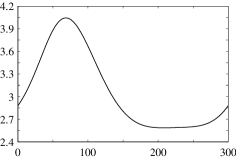
(a)	$\hat{x}$ [mm]

Local film thickness [mm]
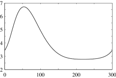
(b)	$\hat{x}$ [mm]

Figure 3: Local film thickness for two different inclination angles. For comparison with [WLA05, Fig. 3] it is measured not perpendicular to the bottom but to the main flow direction $\mathbf{e}_{\hat{x}}$, see Fig. 1. Parameters: $\text{R}=0.0285,\zeta=0.31$ and (a) $\alpha=28^{\circ},\delta=0.059,{\rm B}_{{\rm i}}=2\times 10^{-3}$, (b) $\alpha=18.05^{\circ},$ $\delta=0.068,{\rm B}_{{\rm i}}=3\times 10^{-3}$.

Film thickness [mm]
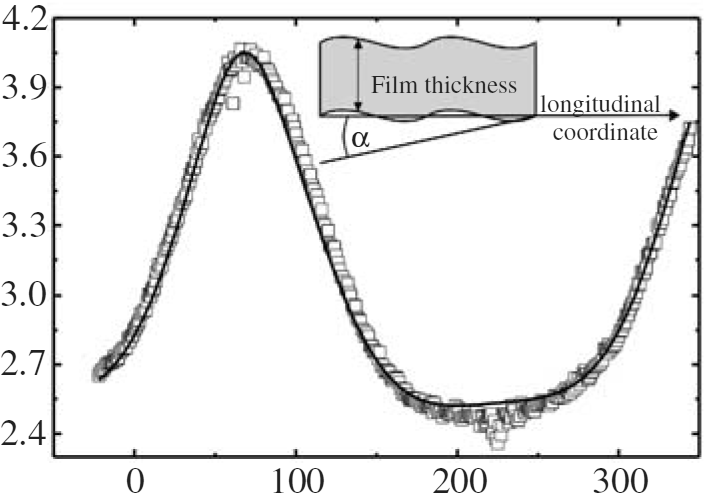
(a)	Longitudinal coordinate [mm]

Film thickness [mm]
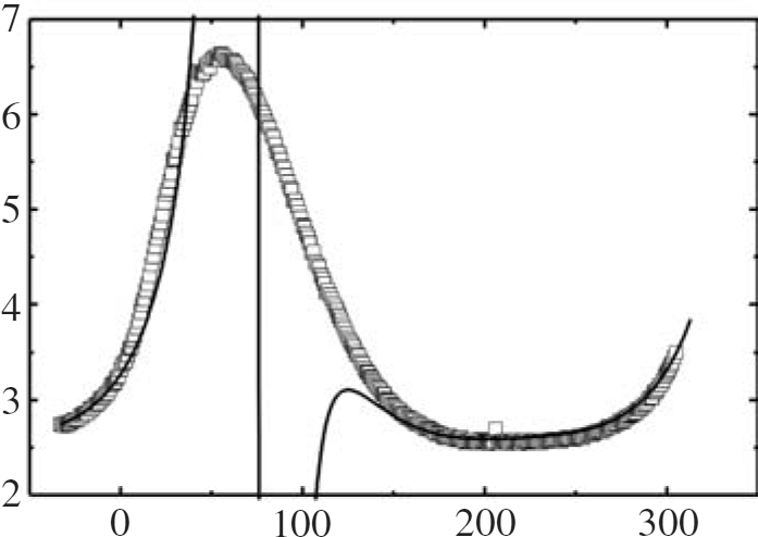
(b)	Longitudinal coordinate [mm]

Figure 4: Experimental data for the parameters used in Fig. 3. Reprint of [WLA05, Fig. 3], with permission from Springer Science+Business Media.

In order to explore wider regimes of parameters and to get more detailed comparison also with full Navier–Stokes numerics we reconstruct the flow field using the second-order profile (47), (48) derived in Appendix B for sinusoidal bottoms. Following [Tri98], see also [Tri07a, Tri07b], we simulate the flow of liquid nitrogen over a vertical sinusoidal bottom with wavelength $\hat{\lambda}=1.57\,\text{mm}$ and amplitude $\hat{a}=0.0875\,\text{mm}$. The fluid parameters are $\nu=$0.182\text{\,}\mathrm{m}{\mathrm{m}}^{2}\mathrm{/}\mathrm{s}$,\rho=$0.808\text{\,}\mathrm{g}\text{\,}{\mathrm{c}}^{-1}\text{\,}{\mathrm{m}}^{3}$$ and $\sigma=$8.87\text{\,}\mathrm{mN}\text{\,}{\mathrm{m}}^{-1}$$ which yield an inverse Bond number ${\rm B}_{{\rm i}}=17.92$. As Reynolds numbers we choose $\text{R}=5$ and $\text{R}=20$. Again we achieve free surface profiles which are in good agreement with the Navier–Stokes numerics in [Tri98, Fig. 10], and also the flow fields are qualitatively and semi-quantitatively reproduced correctly, see Fig. 5 and 6. Namely, there occurs a recirculation zone of correct size in the trough of the bottom contour if the Reynolds number is increased.

$\hat{z}$ [mm]
(a)	$\hat{x}$ [mm]

$\hat{z}$ [mm]
(b)	$\hat{x}$ [mm]

Figure 5: Free surface and reconstructed flow field for stationary solutions of (42), (43) for (a) $\text{R}=5$ and (b) $\text{R}=20$. The other parameters are $\delta=0.15$ respectively $\delta=0.24$, $\alpha=90^{\circ},{\rm B}_{{\rm i}}=17.92,\zeta=0.35,\hat{\lambda}=1.57\,\text{mm}.$

$\hat{z}$ [mm]
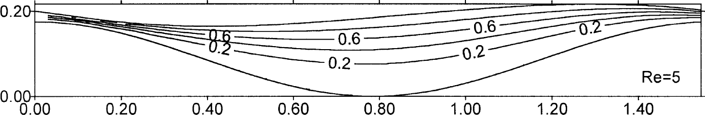
(a)	Distance along gravity [mm]

$\hat{z}$ [mm]
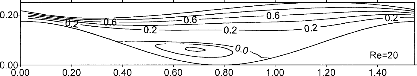
(b)	Distance along gravity [mm]

Figure 6: Full Navier–Stokes numerics for the parameters used in Fig. 5. Reprint of [Tri98, Fig. 10], with permission from Elsevier.

Above we calculated stationary solutions $(F,Q)_{s}$ which, by analogy with the flat bottom case, must be expected to be unstable in the considered regime $(\alpha=90^{\circ})$, see also [WA03, AVB06, Tri07a, Tri07b]. In the following we report on some numerical experiments to investigate the stability of stationary solutions and on some time dependent solutions in the unstable case. The standard approach to study the stability of $(F,Q)_{s}$ would be to calculate the spectrum of the linearization of (42), (43) around $(F,Q)_{s}$, either numerically or analytically by expansion of first the stationary solution and then the eigenvalue problem in suitable small parameters. Eigenvalues of the linearization can then be calculated using Floquet theory. See [Tri07a] for a detailed parametric study of stability using this approach for an IBL, and [Tri07b] for the full Navier–Stokes problem.

Here, since we are mainly interested in the shape of non-stationary bifurcated solutions in case of instability, to determine stability of $(F,Q)_{s}$ we rather use a less systematic ad hoc approach. We numerically calculate $(F,Q)_{s}$ for various R, with fluid and geometry parameters fixed. Then, on a domain with eight bottom undulations, we apply a localized perturbation, let the system run, and determine stability by growth or decay of the perturbations. This yields a critical Reynolds number $\text{R}_{\text{crit}}$ in terms of the remaining parameters.

	A	B	C
$\rho[$\text{\,}\mathrm{g}\text{\,}{\mathrm{c}}^{-1}\text{\,}{\mathrm{m}}^{3}$]$	$0.969$	$0.969$	$1.00$
$\nu[$\text{\,}\mathrm{m}{\mathrm{m}}^{2}\mathrm{/}\mathrm{s}$]$	$24.1$	$24.1$	$1.00$
$\sigma[$\text{\,}\mathrm{mN}\text{\,}{\mathrm{m}}^{-1}$]$	$20.0$	$20.0$	$70.0$
$\hat{\lambda}[$\text{\,}\mathrm{mm}$]$	$108$	$108$	$10.0$
$\alpha[^{\circ}]$	$45$	$10$	$10$
${\rm B}_{{\rm i}}$	$0.01$	$0.04$	$16.2$

Table 2: Parameters used to study stability of stationary solutions, with resulting inverse Bond numbers.

Again we first focus on non-dimensional parameters from [WLA05], namely $\alpha=45^{\circ}$ and ${\rm B}_{{\rm i}}=0.01$, using the dimensional parameter set A from Table 2, and calculate $\text{R}_{\text{crit}}$ as function of $\zeta$, see Fig. 7. In agreement with [WLA05, Fig. 7], see also [AVB06, Tri07b], we find that the wavy bottom strongly increases $\text{R}_{\text{crit}}$ compared to the critical Reynolds number $5/6\cot\alpha$ over flat bottom. In particular, also the quantitative agreement with [WLA05, Fig. 7] is very good. Here the most notable difference between the WRIBL and the rWRIBl occurs: $\text{R}_{\text{crit}}$ is somewhat larger for the WRIBL and hence the rWRIBL appears to be more accurate.

$\text{R}_{\text{crit}}$
	$\zeta$

Figure 7: Critical Reynolds number $\text{R}_{\text{crit}}$ as a function of the waviness $\zeta$ for parameter set A from Table 2. Along the critical values $\delta$ varies from $\delta=0.035$ $(\text{R}=5/6)$ to $\delta=0.048$ $(\text{R}=2.2)$. [WLA05] denotes $\text{R}_{\text{crit}}$ from [WLA05], multiplied by 2/3 due to a different scaling. The critical Reynolds numbers were calculated with a tolerance of $\pm 0.05$.

(a)

(b)

Figure 8: Numerical simulations in the sub- resp. supercritical case for parameter set A from Table 2 and $\zeta=0.5$ which gives $\text{R}_{\text{crit}}\approx 1.4$, cf. Fig. 7; two bottom waves with periodic boundary conditions. (a), $\text{R}=1.1$, $f(\hat{x})$; for larger $t$ the solution relaxes to a stationary solution. (b) $\text{R}=1.6$, $f(\hat{x})$; the solution is unstable and a traveling pulse evolves.

Figure 8 shows time dependent solutions, with $\zeta=0.5$ from Fig. 7, but for graphical reasons with only two bottom undulations. Over flat bottoms, for $\text{R}>\text{R}_{\text{crit}}$ the most prominent solutions are the (experimentally, numerically and analytically well known) traveling pulse trains [CD02]. Also over wavy bottoms pulse like surface waves develop, and the effect of the bottom waviness is a periodic modulation of the amplitude and speed of the pulses: (a) shows the decay of a localized perturbation in the stable case, while (b) shows the emergence of a pulse in the unstable case.

7.2 Some new predictions

The numerics in §7.1 have shown that (42), (43) reproduces known phenomena qualitatively and quantitatively, in particular the appearance of eddies in troughs of the bottom for larger $\zeta$, and the occurrence of a long wave instability when the Reynolds number exceeds a critical value $\text{R}_{\text{crit}}$ as well as the increase of $\text{R}_{\text{crit}}$ with $\zeta$. Next we consider a lower inclination angle for which we again investigate the stability of stationary solutions by the method specified above. Taking the same fluid parameters as in parameter set A but with $\alpha=10^{\circ}$ we get the critical values in Fig. 9 denoted by parameter set B. In contrast to Fig. 7 the critical Reynolds numbers are no longer increasing monotonously but reach a maximum at $\zeta\approx 0.17$. For larger values of the bottom waviness $\text{R}_{\text{crit}}$ decreases, and for $\zeta>0.23$ it becomes less than the critical Reynolds number $5/6\cot\alpha$ for flat bottom.

Next we increase the inverse Bond number by choosing $\hat{\lambda}=10$\text{\,}\mathrm{mm}$$ and the fluid parameters of water, see parameter set C in Table 2 and the resulting critical values in Fig. 9. The dependence on $\zeta$ turns out to be more pronounced than in Fig. 7. Figure 10 shows related time dependent solutions for some supercritical values. For small $\zeta$, e.g. $\zeta=0.04$ in (a), the instability is long wave (pulses), but for $\zeta=0.06$ in (b) the perturbation evolves into a finite wavelength pattern. Thus, for $\alpha=10^{\circ}$ and $\zeta$ larger than a critical value $\zeta_{0}\lesssim 0.06$ there appears a finite wave number instability, and the wave number increases as the bottom waviness becomes larger, see Fig. 10 (c)–(d). Since also the amplitudes of these patterns are very small we conclude on a phenomenological basis that Fig. 10 (b)–(d) shows short wave instabilities, where, however, the following remarks apply.

The linearization of (42), (43) around some $(Q,F)_{s}$ always has a Floquet exponent $\mu_{1}(0)=0$ from conservation of mass. In other words, $\mu_{1}(0)=0$ since we have a family of stationary solutions $(Q,F)_{s}$ parameterized by the total mass $M=\int_{0}^{2\pi}F(1+\frac{1}{2}\delta\zeta KF)d\hat{X}$. If $K\mapsto\mu(K)$ is a parameterization of the Floquet exponents of the linearization by wave number, then short wave instability in a strict sense means that unstable Floquet modes appear only in an interval $\pm K\in(K_{1},K_{2})$ with $K_{1}>0$. However, a finite wave number instability may also be due to a side band (i.e. long wave) instability, that is, a branch $\mu(K)$ of unstable Floquet exponents with Re$\mu(K)=c_{2}K^{2}-c_{4}K^{4}+{\cal O}(K^{6})$ with $c_{2},c_{4}>0$, which up to order $K^{4}$ gives $K_{c}=\sqrt{\frac{c_{2}}{2c_{4}}}$ as the most unstable wave number. To distinguish this from a short wave instability one should actually calculate the spectrum. However, we take (b)–(d) as strong hints for a short wave instability, since if (b)–(d) were due to side band instabilities we would expect larger amplitudes. In any case, to distinguish (a) from (b)–(d) we may call the latter short wave instabilities in a phenomenological sense.

Finally, if $K={\cal O}(1)$ is the wave number of a pattern for the rWRIBL, then $k=\frac{2\pi}{\hat{\lambda}}K$ is the wave number in the dimensional Navier–Stokes system. Thus, if for instance $\hat{h}={\cal O}(1)$ and $\hat{a}={\cal O}(1)$ are fixed such that $\delta=2\pi\hat{h}/\hat{\lambda}={\cal O}(\varepsilon)$ and $\zeta=2\pi\hat{a}/\hat{\lambda}={\cal O}(\varepsilon)$ are small due to $\hat{\lambda}={\cal O}(\varepsilon^{-1})$, then $k={\cal O}(\varepsilon)$. However, even in this case, as already said at the start of §7.1, in applications we always have finite $\varepsilon$. For instance, in Fig. 10 (b)–(d) we find $k=\pi/10,k=\pi/8,k=3\pi/20$ [mm^-1] as the basic wave numbers (the smallest possible wave number over a domain of length 80 mm being $\pi/40$ [mm^-1]).

Over flat bottom, short wave instabilities are only known for very small inclination angles, see [CD02, Section 2.3]. In particular, calculating the eigenvalues of the linearization of the rWRIBL (42), (43) around the Nusselt solution for the above parameters but $\zeta=0$ by a Fourier ansatz we find no short wave instability in case of a flat bottom.

$\text{R}_{\text{crit}}$
	$\zeta$

Figure 9: Critical Reynolds number $\text{R}_{\text{crit}}$ as a function of the waviness $\zeta$ for parameter sets B (${\rm B}_{{\rm i}}=0.04$) and C (${\rm B}_{{\rm i}}=16.2$) from Table 2; for parameter set C the letters a–d indicate the values of $\zeta$ used for the time dependent plots in Fig. 10.

(a)	(b)
(c)	(d)

Figure 10: Time dependent simulations for parameter set C, eight bottom waves, plots of the flow rate $Q$. (a) $\zeta=0.04,\text{R}=7.4$ (long wave instability), (b) $\zeta=0.06,\text{R}=9.7$ (short wave instability, four waves), (c) $\zeta=0.08,\text{R}=9.7$ (short wave instability, five waves), (d) $\zeta=0.2,\text{R}=6.1$ (short wave instability, six waves).

In Fig. 11, for fixed R and varying $\zeta$ we plot the minimal and maximal downstream velocities of some stationary solutions used in Fig. 9, which shows that these are continuations of the Nusselt solution. For $\zeta>\zeta_{1}$ the minimal velocity $u_{\text{min}}$ becomes negative which is an easy diagnostic for the existence of eddies. In particular, from $\zeta_{0}<\zeta_{1}$ we find that the short wave instability sets in before the appearance of eddies, which shows that the short wave instability is an effect of the wavy bottom on a Nusselt like laminar solution. Figure 11 (b) shows the stationary solution and reconstructed streamlines for the short wave unstable parameters $\zeta=0.4,\text{R}=4.2$.

$u$ [mm/s]
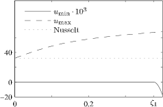
(a)	$\zeta$

$\hat{z}$ [mm]
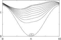
(b)	$\hat{x}$ [mm]

Figure 11: Stationary solutions for parameter set C and $\text{R}=4.2$. (a) Minimal and maximal downstream velocity $u_{\text{min}},u_{\text{max}}$ of stationary solutions depending on $\zeta$. For $\zeta>\zeta_{1}\approx 0.38$ eddies occur. (b) Free surface and reconstructed streamlines for $\zeta=0.4$.

Finally, Fig. 12 illustrates a rather strongly unstable situation where due to a relatively large traveling pulse the free surface is not a graph over $\hat{x}$. This was one of the motivations to use curvilinear coordinates. Downstream the bottom maxima where the local inclination angle is larger than $90^{\circ}$ ($$0\text{\,}\mathrm{mm}$\ {<}\ \hat{x}\ {<}\ $150\text{\,}\mathrm{mm}$$ in Fig. 12) we find a bearing-out of the free surface as a pulse passes. This overhang is typically rather small since the pulse is small as it lost mass when it climbed “uphill” ($$150\text{\,}\mathrm{mm}$\ {<}\ \hat{x}\ {<}\ $300\text{\,}\mathrm{mm}$$ in Fig. 12) to the maximum of the bottom. On the other hand, running “downhill”, the pulse grows and reaches maximum amplitude around $\hat{x}\approx$180\text{\,}\mathrm{mm}$$. This yields an overhang (to the left) of the free surface at the beginning of the “uphill” section.

In the literature we did not find data or solutions comparable to Fig. 12, or to the short wave instability explained in Figures 9 to 11. Thus we think it will be interesting to study either experimentally or by full Navier–Stokes numerics the accuracy of these predictions.

(a)

(b)

Figure 12: $\alpha=90^{\circ}$, $\hat{\lambda}=$300\text{\,}\mathrm{mm}$,\hat{a}=$20\text{\,}\mathrm{mm}$$, hence $\zeta=0.42$, $\text{R}=10$, $\delta=0.32$; ${\rm B}_{{\rm i}}=0.003$ and initial data $(F,Q)\equiv(1,1)$. (a) Free surface over $\hat{x}$, dashed line is the bottom contour. (b) Film thickness $f$ over $\hat{x}$.

7.3 Conclusions

Using a Galerkin method with only one ansatz and test function we derived the WRIBL (31), (32) for film flow over wavy bottom, which in the limit of flat bottom equals the (one-dimensional version of the) WRIBL derived in [SRQM06]. In a second step we regularized the WRIBL to the rWRIBL (42), (43). Numerical simulations of the rWRIBL show very good agreement with available data from experiment and full scale Navier–Stokes numerics. Finally, our rWRIBL predicts two qualitatively new phenomena, namely a short wave instability of Nusselt like solutions (without eddies) at non-small inclination angles and at still rather small $\zeta$, and solutions where the free surface is not a graph over the (Cartesian) downstream coordinate. It remains to be seen whether these predictions can be verified experimentally or by full Navier–Stokes numerics.

Appendix A Curvilinear coordinates

In order to expand the non-dimensional curvature $K$ and the local inclination angle $\theta$ in powers of $\zeta$ we first scale the Cartesian coordinate $\hat{x}$ and the bottom profile $\hat{b}$ by

$$\hat{X}=\frac{2\pi}{\hat{\lambda}}\hat{x},\quad\hat{B}(\hat{X})=\frac{1}{\hat{a}}\hat{b}\left(\frac{\hat{\lambda}}{2\pi}\hat{X}\right).$$

This implies $\partial_{\hat{x}}\hat{b}(\hat{x})=\zeta\partial_{\hat{X}}\!\hat{B}\left(\frac{2\pi}{\hat{\lambda}}\hat{x}\right)$ and $\partial_{\hat{x}}^{2}\hat{b}(\hat{x})=\frac{4\pi^{2}\hat{a}}{\hat{\lambda}^{2}}\partial_{\hat{X}}^{2}\!\hat{B}\left(\frac{2\pi}{\hat{\lambda}}\hat{x}\right).$ The relation between $\hat{X}$ and $X$ is

$$X =\frac{2\pi}{\hat{\lambda}}x=\frac{2\pi}{\hat{\lambda}}\int_{0}^{\hat{x}}\sqrt{1+\left(\partial_{\hat{x}}\hat{b}(\hat{x})\right)^{2}}d\hat{x}$$

$$=\int_{0}^{\hat{X}}\sqrt{1+\zeta^{2}\left(\partial_{\hat{X}}\!\hat{B}(\hat{X})\right)^{2}}d\hat{X}$$

$$=\hat{X}+\frac{1}{2}\zeta^{2}\int_{0}^{\hat{X}}\left(\partial_{\hat{X}}\!\hat{B}(\hat{X})\right)^{2}d\hat{X}+{\cal O}(\zeta^{4}),$$

thus $\hat{X}(X)=X-\frac{1}{2}\zeta^{2}\int_{0}^{X}\left(\partial_{\hat{X}}\!\hat{B}(\hat{X})\right)^{2}d\hat{X}+{\cal O}(\zeta^{4}),$ and therefore $K(X)$ reads (cf. (1))

$$K(X) =\frac{\hat{\lambda}^{2}}{4\pi^{2}\hat{a}}\kappa\left(\frac{\hat{\lambda}}{2\pi}\hat{X}(X)\right)$$

$$=-\frac{\hat{\lambda}^{2}}{4\pi^{2}\hat{a}}\frac{\partial_{\hat{x}}^{2}\hat{b}\left(\frac{\hat{\lambda}}{2\pi}\hat{X}(X)\right)}{\left[1+\left(\partial_{\hat{x}}\hat{b}\left(\frac{\hat{\lambda}}{2\pi}\hat{X}(X)\right)\right)^{2}\right]^{\frac{3}{2}}}=-\frac{\partial_{\hat{X}}^{2}\!\hat{B}(\hat{X}(X))}{\left[1+\zeta^{2}\left(\partial_{\hat{X}}\!\hat{B}(\hat{X}(X))\right)^{2}\right]^{\frac{3}{2}}}$$

$$=-\partial_{\hat{X}}^{2}\!\hat{B}(X)+\frac{1}{2}\zeta^{2}\left(3\partial_{\hat{X}}^{2}\!\hat{B}(X)(\partial_{\hat{X}}\!\hat{B}(X))^{2}+\partial_{\hat{X}}^{3}\!\hat{B}(X)\int_{0}^{X}(\partial_{\hat{X}}\!\hat{B}(\hat{X}))^{2}d\hat{X}\right)+{\cal O}(\zeta^{4})$$

$$=:K_{0}(X)+\zeta^{2}K_{2}(X)+{\cal O}(\zeta^{4}).$$ (44)

For the local inclination angle $\theta$ we get

$$\theta(X) =\arctan\left(\partial_{\hat{x}}\hat{b}\left(\frac{\hat{\lambda}}{2\pi}\hat{X}(X)\right)\right)=\arctan(\zeta\partial_{\hat{X}}\!\hat{B}(\hat{X}(X)))=\zeta\partial_{\hat{X}}\!\hat{B}(X)+{\cal O}(\zeta^{3})$$

$$=:\zeta\theta_{1}(X)+{\cal O}(\zeta^{3}).$$ (45)

Appendix B Second-order velocity profile

Calculating the second-order component of the downstream velocity $U=U_{0}+\varepsilon U_{1}+\varepsilon^{2}U_{2}+{\cal O}(\varepsilon^{3})$ by exactly the same approach as in Section 3 yields

$$\varepsilon^{2}U_{2}=\ \delta^{2}\text{R}^{2}\partial_{X}^{2}\!F\left({-}\frac{27}{4480}FZ^{8}{+}\frac{27}{560}F^{2}Z^{7}{-}\frac{3}{20}F^{3}Z^{6}{+}\frac{9}{40}F^{4}Z^{5}{+}\frac{3}{8}F^{5}Z^{4}{-}\frac{21}{10}F^{6}Z^{3}{+}\frac{30}{7}F^{8}Z\right)$$

$${+}\delta^{2}\text{R}^{2}(\partial_{X}\!F)^{2}\left({-}\frac{27}{4480}Z^{8}{+}\frac{27}{560}FZ^{7}{-}\frac{21}{80}F^{2}Z^{6}{+}\frac{9}{10}F^{3}Z^{5}{+}\frac{15}{8}F^{4}Z^{4}{-}\frac{63}{5}F^{5}Z^{3}{+}\frac{948}{35}F^{7}Z\right)$$

$${+}\delta^{2}\text{R}({\rm B}_{{\rm i}}\partial_{X}^{4}\!F{-}\cot\alpha\ \partial_{X}^{2}\!F)\left(\frac{1}{40}Z^{6}{-}\frac{3}{20}FZ^{5}{+}\frac{3}{4}F^{2}Z^{4}{-}2F^{3}Z^{3}{+}\frac{18}{5}F^{5}Z\right)$$

$${-}\delta\zeta\text{R}({\rm B}_{{\rm i}}\partial_{X}^{2}\!K_{0}{+}\cot\alpha\ \partial_{X}\!\theta_{1})\left(\frac{1}{40}Z^{6}{-}\frac{3}{20}FZ^{5}{+}\frac{3}{8}F^{2}Z^{4}{-}\frac{1}{2}F^{3}Z^{3}{+}\frac{3}{5}F^{5}Z\right)$$

$${+}\delta\text{R}\left(3\delta{\rm B}_{{\rm i}}(\partial_{X}^{2}\!F)^{2}{-}2\delta\cot\alpha(\partial_{X}\!F)^{2}{+}5\delta{\rm B}_{{\rm i}}\partial_{X}^{3}\!F\partial_{X}\!F{-}\zeta({\rm B}_{{\rm i}}\partial_{X}\!K_{0}{+}\cot\alpha\ \theta_{1})\partial_{X}\!F\right)\cdot$$

$$\cdot\left(\frac{3}{4}FZ^{4}{-}3F^{2}Z^{3}{+}6F^{4}Z\right){+}\delta^{2}\text{R}{\rm B}_{{\rm i}}(\partial_{X}\!F)^{2}\partial_{X}^{2}\!F\left(\frac{9}{2}Z^{4}{-}18FZ^{3}{+}36F^{3}Z\right)$$

$${+}\delta\zeta K_{0}\left(\frac{1}{2}Z^{3}{-}\frac{3}{2}FZ^{2}{+}3F^{2}Z\right){+}\delta\zeta\partial_{X}\!\theta_{1}\left({-}\frac{1}{2}Z^{3}{+}\frac{3}{2}FZ^{2}{-}\frac{3}{2}F^{2}Z\right)$$

$${+}\delta^{2}\partial_{X}^{2}\!F\left({-}Z^{3}{-}\frac{3}{2}FZ^{2}{+}\frac{15}{2}F^{2}Z\right){+}\delta\zeta\theta_{1}\partial_{X}\!F\left(\frac{3}{2}Z^{2}{-}3FZ\right)$$

$${+}\delta^{2}(\partial_{X}\!F)^{2}\left({-}\frac{3}{2}Z^{2}{+}15FZ\right){+}\zeta^{2}\theta_{1}^{2}\left(\frac{3}{4}Z^{2}{-}\frac{3}{2}FZ\right).$$ (46)

If the flow rate $Q$ is assumed to be enslaved by the film thickness $F$, then integration of (46) along $Z\in[0,F]$ gives the second-order component of $Q=Q_{0}+\varepsilon Q_{1}+\varepsilon^{2}Q_{2}+{\cal O}(\varepsilon^{3})$, see (34). In order to achieve an accurate velocity profile $\tilde{U}_{2}$ depending on both $F$ and $Q$ we again treat $Q$ as independent ${\cal O}(1)$-quantity. This profile is not needed for the Galerkin method but only for reconstructing flow fields. Therefore we restrict our calculations to the practically relevant case of stationary flow over a sinusoidal bottom $\hat{b}(\hat{x})=\hat{a}\cos\left(\frac{2\pi}{\hat{\lambda}}\hat{x}\right)$. This implies according to (44) and (45)

$$K(X)=\cos X+{\cal O}(\zeta^{2}),\quad\theta(X)=-\zeta\sin X+{\cal O}(\zeta^{3}).$$

In case of the first-order profile (26) the correction of the parabolic profile turned out to be a self-similar polynomial with a coefficient depending on $Q$ and $\partial_{X}\!Q$ but not on $F$ or its spatial derivatives. The basic assumption now is that this is also true for the second-order correction $\tilde{U}_{2}$. Therefore all spatial derivatives of $F$ emanate from $\partial_{X}\!Q$. As we consider here only stationary solutions the evolution equation for $F$ (27) gives $\partial_{X}\!Q=0$. Thus in $U_{2}$ we neglect all terms containing spatial derivatives of $F$. Taking again into account that treating $Q$ as independent quantity mixes up $\varepsilon$-orders in the expansion of $U$ finally yields

$$\varepsilon^{2}\tilde{U}_{2}=\ \delta\zeta\text{R}(\cot\alpha+{\rm B}_{{\rm i}})\cos XQ^{2}\left(\frac{1}{40}\left(\frac{Z}{F}\right)^{6}{-}\frac{3}{20}\left(\frac{Z}{F}\right)^{5}+\frac{1}{4}\left(\frac{Z}{F}\right)^{4}{-}\frac{9}{35}\left(\frac{Z}{F}\right)^{2}+\frac{4}{35}\frac{Z}{F}\right)$$

$$+\delta\zeta\cos XQ\left(\left(\frac{Z}{F}\right)^{3}{-}\frac{3}{4}\left(\frac{Z}{F}\right)^{2}\right).$$

Thus the velocity profile used in Section 7 to reconstruct flow fields reads

$$\tilde{U}=\ \frac{3Q}{F}\left({-}\frac{1}{2}\left(\frac{Z}{F}\right)^{2}+\frac{Z}{F}\right)+\delta\zeta\cos XQ\left(\left(\frac{Z}{F}\right)^{3}{-}\frac{3}{4}\left(\frac{Z}{F}\right)^{2}\right)$$

$$+\delta\zeta\text{R}(\cot\alpha+{\rm B}_{{\rm i}})\cos XQ^{2}\left(\frac{1}{40}\left(\frac{Z}{F}\right)^{6}{-}\frac{3}{20}\left(\frac{Z}{F}\right)^{5}+\frac{1}{4}\left(\frac{Z}{F}\right)^{4}{-}\frac{9}{35}\left(\frac{Z}{F}\right)^{2}+\frac{4}{35}\frac{Z}{F}\right).$$ (47)

The according velocity component $\tilde{W}$ is given by the continuity equation, i.e.

$$\tilde{W}=-\frac{1}{1+\delta\zeta\cos X\ Z}\int_{0}^{Z}\partial_{X}\!UdZ.$$ (48)

Acknowledgement: This work was supported by the DFG under grant Schn 520/6. The authors thank Andreas Wierschem and Vasilis Bontozoglou for stimulating discussions during early stages of this work.

References

- [AVB06] K. Argyriadi, M. Vlachogiannis, and V. Bontozoglou. Experimental study of inclined film flow along periodic corrugations: The effect of wall steepness. Phys. Fluids, 18:012102, 2006.
- [Ben57] T. B. Benjamin. Wave formation in laminar flow down an inclined plane. J. Fluid Mech., 2:554–574, 1957.
- [Ben66] D. J. Benney. Long waves on liquid films. J. of Mathematics and Physics, 45:150–155, 1966.
- [CD02] H.-C. Chang and E. A. Demekhin. Complex Wave Dynamics on Thin Films. Elsevier, Amsterdam, 2002.
- [DO07] L. A. Dávalos-Orozco. Nonlinear instability of a thin film flowing down a smoothly deformed surface. Phys. Fluids, 19:074103, 2007.
- [HBAW09] C. Heining, V. Bontozoglou, N. Aksel, and A. Wierschem. Nonlinear resonance in viscous films on inclined wavy planes. Int. J. Multiphase Flow, 35(1):78–90, 2009.
- [Lin74] S. P. Lin. Finite amplitude side-band stability of a viscous film. J. Fluid Mech., 63(3):417–429, 1974.
- [OGN08] A. Oron, O. Gottlieb, and E. Novbari. Numerical analysis of a weighted-residual integral boundary-layer model for nonlinear dynamics of falling liquid films. European Journal of Mechanics - B/Fluids, 2008. In press.
- [OH08] A. Oron and C. Heining. Weighted-residual integral boundary-layer model for the nonlinear dynamics of thin liquid films falling on an undulating vertical wall. Phys. Fluids, 20:082102, 2008.
- [Oos99] T. Ooshida. Surface equation of falling film flows with moderate Reynolds number and large but finite Weber number. Phys. Fluids, 11(11):3247–3269, 1999.
- [PMP83] A. Pumir, P. Manneville, and Y. Pomeau. On solitary waves running down an inclined plane. J. Fluid Mech., 135:27–50, 1983.
- [PN03] C. D. Park and T. Nosoko. Three-dimensional wave dynamics on a falling film and associated mass transfer. AIChE Journal, 49(11):2715–2727, 2003.
- [Poz88] C. Pozrikidis. The flow of a liquid film along a periodic wall. J. Fluid. Mech., 188:275–300, 1988.
- [RQM98] C. Ruyer-Quil and P. Manneville. Modeling film flows down inclined planes. Eur. Phys. J. B, 6:277–292, 1998.
- [RQM00] C. Ruyer-Quil and P. Manneville. Improved modeling of flows down inclined planes. Eur. Phys. J. B, 15:357–369, 2000.
- [SAB94] T. R. Salamon, R. C. Armstrong, and R. A. Brown. Traveling waves on vertical films – numerical analysis using the finite-element method. Phys. Fluids, 6(6):2202–2220, 1994.
- [Shk67] V. Y. Shkadov. Wave conditions in the flow of a thin layer of a viscous liquid under the action of gravity. Izv. Akad. Nauk. SSSR, Mekh. Zhidk. Gaza, 2:43–51, 1967.
- [SRQM06] B. Scheid, C. Ruyer-Quil, and P. Manneville. Wave patterns in film flows: modelling and three-dimensional waves. J. Fluid Mech., 562:183–222, 2006.
- [Tri98] Y. Y. Trifonov. Viscous liquid film flows over a periodic surface. Int. J. Multiphase Flow, 24(7):1139–1161, 1998.
- [Tri04] Y. Y. Trifonov. Viscous film flow down corrugated surfaces. J. Appl. Mech. and Techn. Phys., 45(3):389–400, 2004.
- [Tri07a] Y. Y. Trifonov. Stability and nonlinear wavy regimes in downward film flows on a corrugated surface. J. Appl. Mech. and Techn. Phys., 48(1):91–100, 2007.
- [Tri07b] Y. Y. Trifonov. Stability of a viscous liquid film flowing down a periodic surface. Intern. J. of Multiphase Flow, 33:1186–1204, 2007.
- [VB02] M. Vlachogiannis and V. Bontozoglou. Experiments on laminar film flow along a periodic wall. J. Fluid Mech., 457:133–156, 2002.
- [VMHM05] O. K. Valluri, G. Matar, F. Hewitt, and M. A. Mendes. Thin film flow over structured packings at moderate Reynolds numbers. Chem. Eng. Sci., 60:1965–1975, 2005.
- [WA03] A. Wierschem and N. Aksel. Instability of a liquid film flowing down an inclined wavy plane. Phys. D, 186(3–4):221–237, 2003.
- [WBH+08] A. Wierschem, V. Bontozoglou, C. Heining, H. Uecker, and N. Aksel. Linear resonance in viscous films on inclined wavy planes. Int. J. Multiphase Flow, 34:580–590, 2008.
- [WLA05] A. Wierschem, C. Lepski, and N. Aksel. Effect of long undulated bottoms on thin gravity-driven films. Acta Mech., 179:41–66, 2005.
- [WSA03] A. Wierschem, M. Scholle, and N. Aksel. Vortices in film flow over strongly undulated bottom profiles at low Reynolds numbers. Phys. Fluids, 15(2):426–435, 2003.
- [Yih63] C. Yih. Stability of liquid flow down an inclined plane. Phys. Fluids, 6(3):321–334, 1963.