Theory of Single File Diffusion in a Force Field

Abstract

The dynamics of hard-core interacting Brownian particles in an external potential field is studied in one dimension. Using the Jepsen line we find a very general and simple formula relating the motion of the tagged center particle, with the classical, time dependent single particle reflection ${\cal R}$ and transmission ${\cal T}$ coefficients. Our formula describes rich physical behaviors both in equilibrium and the approach to equilibrium of this many body problem.

Single file diffusion of a tagged Brownian particle, interacting with other Brownian particles, is a model for motion of a molecule or particle in a crowded one-dimensional environment, such as a biological pore or channel Hanggi ; Eok and for experimentally studied physical systems such as zeolites Hahn and confined colloid particles Lutz ; Haim . The confinement of the tagged particle by the other particles is strong and severely restricts the motion of the particle. The description of this single file motion has been of much theoretical interest Hanggi ; Harris ; Levitt ; Kollmann ; Henk ; Roden ; Taloni ; Tobias ; Aslangul ; Flomenbom . For an infinite system and uniform initial particle density, Harris Harris and Levitt Levitt first showed that a tagged particle exhibits anomalous diffusion $\langle(x_{T})^{2}\rangle\sim t^{1/2}$, rather then normal diffusion $\langle(x_{T})^{2}\rangle\sim t$, due to the strong many body confinement effect. In recent years, two important research direction have begun to emerge. First, the effect of an external force field acting on the particles is important since, in many cases, pores induce entropic barriers Hanggi and are generally inhomogeneous; hence, single file motion in a periodic potential Taloni and a confining box Tobias were investigated. Secondly, initial conditions have a profound effect on single file motion Aslangul ; Flomenbom : for example, particles with initial delta function distribution in space (rather than a uniform distribution as assumed in Harris ; Levitt ) yield normal diffusion Aslangul . This is important since if a potential field is acting on the particles, thermal initial conditions will have a Boltzmann weighting, leading to generally non-uniform initial conditions.

Here we provide a general and surprisingly simple theory of single file diffusion valid in the presence (or absence) of a potential field, $V(x)$, as well as for thermal and non-thermal initial conditions. In addition, we briefly discuss why our main results are valid even for the case where the underlying dynamics is anomalous remark1 . Our general result reproduces those previously obtained as well as many new ones, by mapping the many particle problem onto a solvable single particle model.

In our model, $2N+1$ identical particles with hard core particle-particle interactions are undergoing Brownian motion in one dimension, so particles cannot pass one another. An external potential field $V(x)$ is acting on the particles. We tag the central particle, which has $N$ other particles to its left, and $N$ to its right. Initially the tagged particle is at $x=0$. The motion of a single particle, in the absence of interactions with other particles, is over-damped Brownian motion so that the single non interacting particle Green function $g(x,x_{0},t)$, with the initial condition $g(x,x_{0},0)=\delta(x-x_{0})$, is obtained from the Fokker-Planck equation Risken

$${\partial g(x,x_{0},t)\over\partial t}=D\left[{\partial^{2}\over\partial x^{2}}-{1\over k_{b}T}{\partial\over\partial x}F\left(x\right)\right]g(x,x_{0},t),$$ (1)

and $F(x)=-V^{\prime}(x)$ is the force field.

In Fig. 1 a schematic diagram of the problem is presented. The straight line is called the Jepsen line, which starts from the origin $x=0$ and follows the rule $x(t)=vt$, where $v$ is a test velocity Levitt . In the interacting system we label particles according to their initial position increasing to the right (see Fig. 1). As noticed in Jepsen ; Levitt , since the Brownian particles are impermeable, every time a particle crosses the Jepsen line from the right (or left), the particle number immediately to the left of the line will be raised (or lowered) by one, respectively. Hence, the particle number immediately to the left of the Jepsen line defines a stochastic process decreasing and increasing its value $+1$ or $-1$ or zero randomly.

Following Levitt Levitt we now consider a non interacting system, equivalent to the interacting one in the large $N$ limit. We let particles pass through each other, but switch labels upon collision, and introduce the counter $\alpha(t)$ which increases by $+1$ if a particle crosses the Jepsen line from left, and decreases by $-1$ when a particle crosses this line from right. The event when the counter $\alpha$ has the value zero, is equivalent to finding the tagged particle to the left of the Jepsen line in the interacting system. This is the case since then the total number of crossings from left to right is equal the number of crossings from right to left. So the probability of the tagged particle being in the vicinity of $x_{T}=vt$ is given by the probability that $\alpha=0$, i.e. by the statistics of the number of transitions of the Jepsen line Levitt . In what follows we depart from the approach in Levitt ; remark3 .

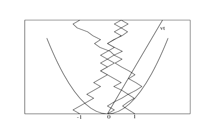
Figure 1: Schematic motion of Brownian particles in a harmonic potential (the parabola) where particles cannot penetrate through each other. The straight line is called the Jepsen line, as explained in the text. The center tagged particle is labeled $0$. In an equivalent non-interacting picture, we allow particles to pass through each other, and we follow the trajectory of the particle which is at the center.

Our aim is to calculate the probability of the random variable $\alpha$, $P_{N}(\alpha)$, and then switch $vt\to x_{T}$ to find the probability density function (PDF) of the tagged particle. For that we designate $P_{LL}(x_{0}^{-j})$ as the probability that a non tagged particle $j$ starting to the left of the Jepsen line $x_{0}^{-j}<0$, is found also at time $t$ on the left of this line. $P_{LR}$ is the probability of a particle starting to the left of the Jepsen line to end on the right, and similarly for $P_{RR}$ and $P_{RL}$. Consider first $N=1$, that is, one particle which starts at $x_{0}^{1}>0$ and a second particle which starts at $x_{0}^{-1}<0$. Then clearly we have either $\alpha=\pm 1$ or $\alpha=0$. The probabilities of these events are easily calculated, for example $P_{N=1}\left(\alpha=1\right)=P_{LR}(x_{0}^{-1})P_{RR}(x_{0}^{+1})$ is the probability that one particle crossed from $L$ to $R$ and the other remained in domain $R$. Similarly $P_{N=1}\left(\alpha=0\right)=P_{LL}(x_{0}^{-1})P_{RR}(x_{0}^{+1})+P_{LR}(x_{0}^{-1})P_{RL}(x_{0}^{+1})$ and $P_{N=1}(\alpha=-1)=P_{LL}(x_{0}^{-1})P_{RL}(x_{0}^{+1})$. Since in the non-interacting picture, the motion of the particles are independent, we can use random walk theory and Fourier analysis Montroll to find the behavior for any $N$

$$P_{N}\left(\alpha\right)={1\over 2\pi}\int_{-\pi}^{\pi}{\rm d}\phi\Pi_{j=1}^{N}\lambda\left(\phi,x_{0}^{-j},x_{0}^{j}\right)e^{i\alpha\phi}.$$ (2)

Where the structure function is

$$\lambda\left(\phi,x_{0}^{-j},x_{0}^{j}\right)=e^{i\phi}P_{LR}(x_{0}^{-j})P_{RR}(x_{0}^{j})+P_{LL}(x_{0}^{-j})P_{RR}(x_{0}^{j})$$

$$+P_{LR}(x_{0}^{-j})P_{RL}(x_{0}^{j})+e^{-i\phi}P_{LL}(x_{0}^{-j})P_{RL}(x_{0}^{j}).$$ (3)

We average Eq. (2) with respect to the initial conditions $x_{0}^{j}$ and $x_{0}^{-j}$, which are assumed to be independent identically distributed random variables and we find

$$\langle P_{N}\left(\alpha\right)\rangle={1\over 2\pi}\int_{-\pi}^{\pi}{\rm d}\phi\langle\lambda\left(\phi\right)\rangle^{N}e^{i\alpha\phi}$$ (4)

where from Eq. (3) the averaged structure function is

$$\langle\lambda\left(\phi\right)\rangle=$$

$$e^{i\phi}\langle P_{LR}\rangle\langle P_{RR}\rangle+\langle P_{LL}\rangle\langle P_{RR}\rangle+\langle P_{LR}\rangle\langle P_{RL}\rangle+e^{-i\phi}\langle P_{LL}\rangle\langle P_{RL}\rangle.$$ (5)

The averages in Eq. (5) are easy to find in principle, in terms of the Green function of the non-interacting particle and the initial density of particles, for example

$$\langle P_{LR}\rangle=\int_{-\overline{L}}^{0}f_{L}(x_{0})\int_{x_{T}}^{\overline{L}}g(x,x_{0},t){\rm d}x{\rm d}x_{0}$$ (6)

where the mentioned replacement $vt\to x_{T}$ was made. Here $f_{L}(x_{0})$ is the PDF of initial positions of the particles which initially are at $x_{0}<0$, similarly $f_{R}(x_{0})$ describes the initial conditions of the right particles. In Eq. (6) $\overline{L}$ is the system size, which can be taken to infinity in the usual way.

Eq. (4) describes a random walk where the number of particles $N$ serves as an operational time. We may use the Gaussian central limit theorem (CLT) to analyze this walk, when $N\to\infty$. In that limit the first two moments of the structure function, $\mu_{1}$ and $\mu_{2}$, found in the small $\phi$ expansion

$$\langle\lambda(\phi)\rangle=1+i\mu_{1}\phi-{1\over 2}\mu_{2}\phi^{2}+O(\phi^{3})$$ (7)

are the only two parameters needed to determine the behavior of $P_{N}(\alpha)$. Defining the variance $\sigma^{2}=\mu_{2}-(\mu_{1})^{2}$, using Eq. (5) and the normalization condition e.g. $\langle P_{LR}\rangle+\langle P_{LL}\rangle=1$ we find the expected result

$$\mu_{1}=\langle P_{LR}\rangle-\langle P_{RL}\rangle$$ (8)

$$\sigma^{2}=\langle P_{RR}\rangle\langle P_{RL}\rangle+\langle P_{LL}\rangle\langle P_{LR}\rangle.$$ (9)

Using the CLT we have the probability of zero crossing, namely $\alpha=0$ in the $N\to\infty$ limit

$$P_{N}\left(\alpha=0\right)\sim{\exp\left(-{N(\mu_{1})^{2}\over 2\sigma^{2}}\right)\over\sqrt{2\pi N}\sigma}.$$ (10)

This is our first general result, valid for a large class of Green functions and initial conditions and thus suited for the investigation of a wide range of problems.

Symmetric potential fields $V(x)=V(-x)$, and symmetric initial conditions are now investigated. The latter simply means that the density of the initial positions of the left particles, i.e. those residing initially in $x_{0}<0$, is the same as that of the right particles, $f_{R}(x_{0})=f_{L}(-x_{0})$. In this case the subscript $R$ and $L$ is redundant and we use $f(x_{0})=f_{R}(x_{0})=f_{L}(-x_{0})$ to describe the initial conditions remark4 . From symmetry it is clear that the tagged particle is unbiased, namely $\langle x_{T}\rangle=0$. Further, since $N$ is large we may expand expressions in the $\exp$ in Eq. (10) in $x_{T}$, to obtain leading terms

$$\mu_{1}=\Delta Jx_{T}+O(x_{T})^{2}$$ (11)

where we used the symmetry of the problem which implies $(\langle P_{LR}\rangle-\langle P_{RL}\rangle)_{x_{T}=0}=0$, and by definition

$$\Delta J={\partial\over\partial x_{T}}\left[\langle P_{LR}(x_{T})\rangle-\langle P_{RL}\left(x_{T}\right)\rangle\right]|_{x_{T}=0}.$$ (12)

Similarly

$$\sigma^{2}=2\langle P_{RR}(x_{T})\rangle\left[1-\langle P_{RR}\left(x_{T}\right)\rangle\right]|_{x_{T}=0}+O(x_{T}).$$ (13)

We designate $\langle P_{RR}(x_{T})\rangle|_{x_{T}=0}={\cal R}$ as a reflection coefficient, since it is the probability that a particle starting at $x_{0}<0$ is found at $x<0$ at time $t$ when an average over all initial conditions is made

$${\cal R}=\int_{0}^{\overline{L}}f(x_{0})\int_{0}^{\overline{L}}g(x,x_{0},t){\rm d}x{\rm d}x_{0}.$$ (14)

As usual the transmission coefficient ${\cal T}=1-{\cal R}$ is defined through ${\cal T}=\langle P_{RL}(x_{T})\rangle|_{x_{T}=0}$. Notice that these reflection and transmission coefficients are time dependent single particle quantities which give useful information for the many body problem. Also from symmetry we have ${\partial\over\partial x_{T}}\langle P_{RL}(x_{T})\rangle|_{x_{T}=0}=-{\partial\over\partial x_{T}}\langle P_{LR}(x_{T})\rangle|_{x_{T}=0}$ in Eq. (12). Hence we define $j=-\partial\langle P_{LR}(x_{T})\rangle/\partial x_{T}|_{x_{T}=0}$ where from its definition Eq. (6)

$$j=\int_{0}^{\overline{L}}f(x_{0})g(0,x_{0},t){\rm d}x_{0}.$$ (15)

So $j$ is the density of non-interacting particles at $x=0$ for an initial density $f(x_{0})$. Using Eqs. (10-13) we find our main result the PDF of the tagged particle

$$P(x_{T})\sim{1\over\sqrt{2\pi\langle\left(x_{T}\right)^{2}\rangle}}\exp\left[-{\left(x_{T}\right)^{2}\over 2\langle\left(x_{T}\right)^{2}\rangle}\right]$$ (16)

where $\langle\left(x_{T}\right)^{2}\rangle={\cal R}{\cal T}/(2Nj^{2})$ is the mean square displacement (MSD).

Gaussian packet. As our first example, we consider particles without external forces $V(x)=0$, in an infinite system with symmetric Gaussian initial conditions with a width $\xi$: $f(x_{0})=\sqrt{2}\exp(-x_{0}^{2}/(2\xi^{2})))/\sqrt{\pi\xi^{2}}$ $(x_{0}>0)$. The free particle Green function is

$$g(x,x_{0},t)={\exp\left(-{(x-x_{0})^{2}\over 4Dt}\right)\over\sqrt{4\pi Dt}}.$$ (17)

Using Eqs. (14-17) we find the MSD of the tagged particle remark

$$\langle(x_{T})^{2}\rangle\sim\xi^{2}{\pi\over N}\left(1+{2Dt\over\xi^{2}}\right)\left[{1\over 4}-{1\over\pi^{2}}\mbox{arccot}^{2}\left(\sqrt{{2Dt\over\xi^{2}}}\right)\right].$$ (18)

This solution exhibits a transition from anomalous sub-diffusion to normal diffusion. At short times $2Dt/\xi^{2}\ll 1$ $\langle(x_{T})^{2}\rangle\sim\xi{\sqrt{2Dt}\over N}$ while at long times $\langle(x_{T})^{2}\rangle\sim{\pi Dt\over 2N}$. For short times the particles do not have time to disperse, hence the motion of the tagged particle is slower than normal, increasing as $t^{1/2}$ since it is confined by the other particles in the system.

Particles in a box. We now consider the example of particles in a box extending from $-\overline{L}$ to $\overline{L}$, which was recently investigated using the Bethe–ansatz and numerical simulations Tobias . The tagged particle initially on $x=0$ has $N$ particles uniformly distributed to its left and similarly to its right. In this case $f(x_{0})=1/\overline{L}$ for $0<x_{0}<\overline{L}$. The green function $g(x,x_{0},t)$ of a single particle in a box with reflecting walls is found using an eigenvalue approach Risken , similar to the method of solution of the undergraduate quantum mechanical problem of a particle in a box. We find

$${\cal R}={1\over 2}+{4\over\pi^{2}}\sum_{n=1,\mbox{Odd}}^{\infty}{\exp\left[-D{\left(\pi^{2}n^{2}\right)\over 4\overline{L}^{2}}t\right]\over n^{2}}$$ (19)

so at $t=0$, ${\cal R}=1$ since all particles initially say in $(0,\overline{L})$ did not have time to move to the other side of box, and $\lim_{t\to\infty}{\cal R}=1/2$ since in the long time limit there is equal probability for a non-interacting particle to occupy half of the box. The eigenvalues of the non-interacting particle control the exponential decay of ${\cal R}$ Eq. (19) which in turn determines the dynamics of the interacting tagged particle. We also find $j=1/2\overline{L}$ using Eq. (15). For short times $D\pi^{2}t/4\overline{L}^{2}\ll 1$ we can replace the summation in Eq. (19) with integration and then using Eq. (16) and $\rho=N/\overline{L}$

$$P\left(x_{T}\right)\sim{\sqrt{\rho}\over 2\left(\pi Dt\right)^{1/4}}\exp\left[-{\rho\left(x_{T}\right)^{2}\sqrt{\pi}\over 4\sqrt{Dt}}\right].$$ (20)

Thus the tagged particle undergoes a single file sub-diffusive process Harris ; Levitt $\langle(x_{T})^{2}\rangle\sim 2(Dt)^{1/2}/(\rho\sqrt{\pi})$, since for short times the particles do not interact with walls. In the long time limit, the tagged particle reaches an equilibrium easily found using Eqs. (16,19)

$$p\left(x_{T}\right)\sim{\sqrt{N}\over\sqrt{\pi}\overline{L}}e^{-{N(x_{T})^{2}\over\overline{L}^{2}}}$$ (21)

and $\lim_{t\to\infty}\langle(x_{t})^{2}\rangle=\overline{L}^{2}/(2N)$. More generally from Eq. (16), $\langle(x_{T})^{2}\rangle=2{\cal R}\left(1-{\cal R}\right)\overline{L}^{2}/N$ which nicely matches and simplifies considerably, the Bethe-ansatz solution Tobias already for $N=70$ remark5 .

Thermal initial conditions. If we assume that initially the particles are in thermal equilibrium, our simple formulas simplify even more. If $f(x_{0})=2\exp(-V(x_{0})/k_{b}T)/Z$ where the normalizing partition function is

$$Z=\int_{-\infty}^{\infty}\exp\left[-{V\left(x\right)\over k_{b}T}\right]{\rm d}x$$ (22)

then $j=1/Z$. To see this, note that since we have a symmetric case $V(x)=V(-x)$ then $g(0,-x_{0},t)=g(0,x_{0},t)$ and $j=2\int_{0}^{\infty}\exp\left[-V(x_{0})/k_{b}T\right]g(0,x_{0},t){\rm d}x_{0}/Z$ gives

$$j=\int_{-\infty}^{\infty}{\exp\left[-{V\left(x_{0}\right)\over k_{b}T}\right]\over Z}g(0,x_{0},t){\rm d}x_{0}.$$ (23)

Where we assume that the potential is binding so a stationary solution of the Fokker-Planck equation is reached i.e. free particle Eq. (17) is excluded. Therefore $j$ Eq. (23) is the probability of finding non-interacting particles on the origin, with thermal equilibrium initial conditions. Since the latter is the stationary solution of the Fokker-Planck operator, $j$ is time independent and equal to $j=\exp[-V(0)/k_{b}T]/Z$. We can always choose $V(0)=0$ and then $j=1/Z$. Using Eq. (16) we find the MSD of the tagged particle

$$\langle(x_{T})^{2}\rangle={{\cal R}{\cal T}Z^{2}\over 2N}.$$ (24)

Single file motion in Harmonic Potential. We now consider particles in an Harmonic potential field $V(x)=m\omega^{2}x^{2}/2$ where $\omega$ is the Harmonic frequency and initially the particles are in thermal equilibrium. The corresponding single particle green function $g(x,x_{0},t)$ describes the Ornstein–Uhlenbeck process, and is well known Risken . Defining the thermal length scale $\xi_{{\rm th}}=\sqrt{k_{b}T/m\omega^{2}}$ and using thermal initial conditions $f(x_{0})=\sqrt{2/\pi\xi_{{\rm th}}^{2}}\exp\left[-(x_{0})^{2}/2\xi_{{\rm th}}^{2}\right]$, we find using Eqs. (14,22,24)

$$\langle\left(x_{T}\right)^{2}\rangle={\pi\over N}\left(\xi_{{\rm th}}\right)^{2}\left\{{1\over 4}-{1\over\pi^{2}}\mbox{arccot}^{2}\left[\sqrt{\exp\left(2\tilde{t}\right)-1}\right]\right\}$$ (25)

where $\tilde{t}=Dt/(\xi_{{\rm th}})^{2}$ is dimensionless time. For short times $\tilde{t}\ll 1$ we obtain sub-diffusive behavior $\langle(x_{T})^{2}\rangle\sim\xi_{{\rm th}}\sqrt{2Dt}/N$ since then the effects of the binding field are negligible, while the tagged particle motion is restricted by all others leading to sub-diffusive behavior. For long times the tagged particle reaches an equilibrium $\langle(x_{T})^{2}\rangle\sim\pi(\xi_{{\rm th}})^{2}/4N$.

Equilibrium of tagged particle. In the long time limit, and for binding potential fields we find again a simple limiting behavior. First, note that $\lim_{t\to\infty}{\cal R}=1/2$ as is easily obtained from Eq. (14) and physically obvious for the symmetric system under investigation. Secondly, for any initial condition $g(0,x_{0},t)=1/Z$ when $t\to\infty$, namely the Green function reached an equilibrium and hence we find from Eq. (15) $\lim_{t\to\infty}j=1/Z$. Therefore in the long time limit

$$\lim_{t\to\infty}\langle\left(x_{T}\right)^{2}\rangle\sim{Z^{2}\over 8N}.$$ (26)

Consistently, this result can be derived directly from the canonical ensemble, using the many body Hamiltonian of the system, in the large $N$ limit, without resorting to dynamics as we did here. The long time limit of our examples of particles in a box Eq. (21) and in a harmonic field Eq. (25) are easily recovered from the more general Eq. (26).

In the examples analyzed so far, we considered symmetric external fields, and initial conditions, which yield no drift $\langle x_{T}\rangle=0$. Our general results Eqs. (10,16) can be extended to cases where the drift is non-zero, then expansions Eqs. (11,12,13) include additional terms which make the final expression slightly more cumbersome and hence suited for a longer publication. Another interesting extension of this work is the case where the particle dynamics, in the absence of interactions with each other, is anomalous as was considered in Flomenbom ; Band for the case of sub-diffusing particles remark1 . These results will be addressed in the future.

To conclude, we have mapped the many body problem of interacting hard core Brownian particles to a single particle problem where calculation of the reflection coefficient ${\cal R}$ and $j$ yield the motion of the tagged particle. In the large $N$ limit, information on the motion of the tagged particle is contained in the single particle Green function $g(x,x_{0},t)$ which can be calculated with known methods. Rich physical behaviors emerge, which depend on the initial distribution of the particles and the force field. For particles in a confining field, a transition from sub-diffusion behavior to an equilibrium value is found to be controlled by the eigen modes of the single particle green function, thus the approach to equilibrium is fast in this sense, even though the diffusion is slower than normal. In contrast, for Gaussian initial conditions a transition between sub-diffusive to normal diffusion is found, which is the expected transition for a wide variety of well behaved initial conditions in the absence of a force. The most rewarding part of this work are the simple equations we find for the single file problem.

Acknowledgments EB is supported by the Israel Science foundation. We thank Tobias Ambjörnsson for helpful discussions.

References

- (1) P.S. Burada, P. Hänggi, F. Marchesoni G. Schmid, and P. Talkner arXiv:0808.2345v1 [cond-mat.stat-mech] (2008).
- (2) H. Kim, C. Kim, E. K. Lee, P. Talkner, and P. Hänggi Phys. Rev. E 77, 031202 (2008).
- (3) K. Hahn, J. Kärgeri, and V. Kukla Phys. Rev. Lett. 76 2762 (1996).
- (4) C. Lutz, M. Kollmann, and C. Bechinger Phys. Rev. Lett. 93 026001 (2004).
- (5) B. Lin, M. Meron, B. Cui, S. A. Rice, H. Diamant Phys. Rev. Lett. 94 216001 (2005).
- (6) T. E. Harris J. Appl. Prob. 2, 323 (1965).
- (7) D. G. Levitt Phys. Rev. A 8 3050 (1973).
- (8) M. Kollmann Phys. Rev. Lett. 90 180602 (2003).
- (9) H. van Beijeren, K. W. Kehr, and R. Kutner Phys. Rev. B 28 5711 (1983).
- (10) C. Rödenbeck, J. Kärger, and K. Hahn Phys. Rev. E 57 4382 (1998).
- (11) A. Taloni, and F. Marchesoni Phys. Rev. Lett. 96, 020601 (2006).
- (12) L. Lizana, T. Ambjörnsson Phys. Rev. Lett. 100, 200601 (2008).
- (13) Cl. Aslangul Europhysics Letters 44 284 (1998).
- (14) O. Flomenbom, and A. Taloni Europhysics Letters 83 20004 (2008).
- (15) Physically this might be important for dynamics in slit pores, where it was shown that non-interacting particles, exhibit super-diffusion, due to forward scattering from the walls of pore Eok .
- (16) H. Risken The Fokker-Planck Equation Springer-Verlag (Berlin) (1984).
- (17) D. W. Jepsen J. Math. Phys. (N.Y) 6 405 (1965).
- (18) Levitt Levitt uses a Poissonian approximation to calculate the motion of a tagged particle in the absence of a potential field. We find that for our aim, where an external force is acting on the particles, the Poissonian approximation is wrong. This can be shown by an exact calculation of the equilibrium distribution of the tagged particle, using Boltzmann-Gibbs canonical ensemble.
- (19) E. W. Montroll and B. J. West in Fluctuation Phenomena E. W. Montroll and J. L. Lebowitz Editors, Studies in Statistical Mechanics Vol. VII North Holland, Amsterdam (1979).
- (20) if , and .
- (21) To obtain Eq. (18) we need the following integral .
- (22) We compared our analytical result with simulations of Tobias in Fig. 4.
- (23) T. Bandyopadhyay Europhysics Letters 81 16003 (2008).