Computing Irreducible Decomposition of Monomial Ideals

Abstract.

The paper presents two algorithms for finding irreducible decomposition of monomial ideals. The first one is recursive, derived from staircase structures of monomial ideals. This algorithm has a good performance for highly non-generic monomial ideals. The second one is an incremental algorithm, which computes decompositions of ideals by adding one generator at a time. Our analysis shows that the second algorithm is more efficient than the first one for generic monomial ideals. Furthermore, the time complexity of the second algorithm is at most $O(n^{2}p\ell)$ where $n$ is the number of variables, $p$ is the number of minimal generators and $\ell$ is the number of irreducible components. Another novelty of the second algorithm is that, for generic monomial ideals, the intermediate storage is always bounded by the final output size which may be exponential in the input size.

1. Introduction

Monomial ideals provide ubiquitous links between combinatorics and commutative algebra [24, 16]. Though simple they carry plentiful algebraic and geometric information of general ideals. Our interest in monomial ideals is motivated by a paper of [9], where they studied the connection between the structure of monomial basis and the geometric structure of the solution sets of zero-dimensional polynomial ideals. Irreducible decomposition of monomial ideals is a basic computational problem and it finds applications in several areas, ranging from pure mathematics to computational biology, see for example [12] for computing integer programming gaps, [3] for computing tropical convex hulls, [22] for finding the joins and secant varieties of monomial ideals, [2] for partition of a simplicial complex, [19] for solving the Frobenius problem, and [13] for modeling gene networks.

We are interested in efficient algorithms for computing irreducible decomposition of monomial ideals. There are a variety of algorithms available in the literature. The so-called splitting algorithm: Algorithm 3.1.2 in [23] is not efficient on large scale monomial ideals. [17] gives two algorithms: one is based on Alexander duality [14], and the other is based on Scarf complex [4]. [18] improves the Scarf complex method by a factor of up to more than 1000. Recently, [20] proposed several slicing algorithms based on various strategies.

Our goals in this paper are to study the structure of monomial ideals and present two new algorithms for irreducible decomposition. We first observe some staircase structural properties of monomial bases in Section 4. The recursive algorithm presented in Section 5 is based on these properties, which allow decomposition of monomial ideals recursively from lower to higher dimensions. This algorithm was presented as posters in ISSAC 2005 and in the workshop on Algorithms in Algebraic Geometry at IMA in 2006. Our algorithm was recently generalized by [20] where several cutting strategies were developed and our algorithm corresponds to the minimum strategy there. Also, the computational experiments there shows that our algorithm has good performance for most cases, especially for highly non-generic monomial ideals.

Our second algorithm is presented in Section 6. It can be viewed as an improved Alexander dual method ([14, 17]). It is incremental based on some distribution rules for “$+$” and “$\cap$” operations of monomial ideals. We maintain an output list of irreducible components, and at each step we add one generator and update the output list. In [17], there is no specific criterion for selecting candidates that need to be updated, and the updating process is inefficient too. Our algorithm avoids these two deficiencies. Our analysis in Section 7 shows that the second algorithm works more efficiently than the first algorithm for generic monomial ideals. We prove that, for generic monomial ideals, the intermediate storage size (ie. number of irreducible components at each stage) is always bounded by the final output size, provided that the generators are added in lex order. This enables us to show that the time complexity of the second algorithm is at most $O(n^{2}p\ell)$ where $n$ is the number of variables, $p$ is the number of minimal generators and $\ell$ is the number of irreducible components.

In Section 2, we present some notations and introductory materials on monomial ideals. In Section 3 we discuss tree representations and operations of monomial ideals.

2. Monomial Ideals

We refer the reader to the books of [5] for background in algebraic geometry and commutative algebra, and to the monograph [16] for monomial ideals and their combinatorial properties.

Let $\mathbb{K}$ be a field and $\mathbb{K}[X]$, the polynomial ring over $\mathbb{K}$ in $n$ indeterminates $X=x_{1},\ldots,x_{n}$. For a vector $\alpha=(a_{1},\ldots,a_{n})\in\mathbb{N}^{n}$, where $\mathbb{N}=\{0,1,2,\ldots\}$ denotes the set of nonnegative integers, we set

$$X^{\alpha}=x_{1}^{a_{1}}\ldots x_{n}^{a_{n}},$$

which is called a monomial. Thus monomials in $n$ variables are in $1-1$ correspondence with vectors in $\mathbb{N}^{n}$. Suppose $\alpha=(a_{1},\ldots,a_{n})$ and $\beta=(b_{1},\ldots,b_{n})$ are two vectors in $\mathbb{N}^{n}$, we say

$$\alpha\leq\beta\textrm{ if }a_{j}\leq b_{j}\textrm{ for all }1\leq j\leq n.$$

This defines a partial order on $\mathbb{N}^{n}$, which corresponds to division order for monomials since $x^{\alpha}|x^{\beta}$ if and only if $\alpha\leq\beta$. We say

$$\alpha<\beta\textrm{ if }\alpha\leq\beta\textrm{ but }\alpha\neq\beta.$$

Also we define

$$\alpha\prec\beta\textrm{ if }a_{j}<b_{j}\textrm{ for all }1\leq j\leq n.$$

Then $\alpha\nprec\beta$ means that $a_{j}\geq b_{j}$ for at least one $j$.

An ideal $I\subset\mathbb{K}[X]$ is called a monomial ideal if it is generated by monomials. Dickson’s Lemma states that every monomial ideal in $\mathbb{K}[X]$ has a unique minimal set of monomial generators, and this set is finite. Denote this set to be $\mbox{Min}(I)$, that is,

$$\mbox{Min}(I)=\{X^{\alpha}\in I:\textrm{ there is no }X^{\beta}\in I\ \textrm{ such that }\beta<\alpha\}.$$

A monomial ideal $I$ is called Artinian if $I$ contains a power of each variable, or equivalently, if the quotient ring $\mathbb{K}[X]/I$ has finite dimension as vector space over $\mathbb{K}$. For convenience of notations, we define

$$x_{i}^{\infty}=0,\quad 1\leq i\leq n.$$

By adding infinity power of variables if necessary, a non-Artinian monomial ideal can be treated like an Artinian monomial ideal. For example, $I=\langle x^{2}y^{3}\rangle=\langle x^{\infty},x^{2}y^{3},y^{\infty}\rangle$. Instead of adding infinity powers, we can also add powers $x_{i}^{c_{i}}$ where $c_{i}$ is a sufficiently large integer, say larger than the largest degree of $x_{i}$ in all the monomials in $\mbox{Min}(I)$. Then the irreducible components of the original ideal are in 1-1 correspondence to those of the modified Artinian ideal; See Exercise 5.8 in [16] or Proposition 3 in [20]. In our algorithms belows, we will use infinity powers, but in the proofs of all the results, we will use powers $x_{i}^{c_{i}}$.

An ideal $J\subset\mathbb{K}[X]$ is called irreducible if it can not be expressed as the intersection of two strictly larger ideals in $\mathbb{K}[X]$. That is, $J=J_{1}\cap J_{2}$ implies that $J=J_{1}$ or $J=J_{2}$. A monomial ideal $I$ is irreducible if and only if $I$ is of the form

$$m^{\beta}=\langle x_{1}^{b_{1}},\ldots,x_{n}^{b_{n}}\rangle$$

for some vector $\beta=(b_{1},\ldots,b_{n})\in\overline{\mathbb{N}}^{n}$ where $\overline{\mathbb{N}}=\mathbb{N}\cup\{\infty\}\setminus\{0\}$. Thus irreducible monomial ideals are in 1-1 correspondence with $\beta\in\overline{\mathbb{N}}^{n}$.

An irreducible decomposition of a monomial ideal $I$ is an expression of the form

$$I=m^{\beta_{1}}\cap\cdots\cap m^{\beta_{r}}$$ (1)

where $\beta_{1},\ldots,\beta_{r}\in\overline{\mathbb{N}}^{n}$. Since the polynomial ring $\mathbb{K}[X]$ is Noetherian, every ideal can be written as irredundant intersection of irreducible ideals. Such an intersection is not unique for a general ideal, but unique for a monomial ideal. We say that the irreducible decomposition (1) is irredundant if none of the components can be dropped from the right hand side. If (1) is irredundant, then the ideals $m^{\beta_{1}},\ldots,m^{\beta_{r}}$ are called irreducible components of $I$. We denote by ${\mbox{Irr}(I)}$ the set of exponents of irreducible components of $I$, that is,

$$\mbox{Irr}(I)=\{\beta_{1},\ldots,\beta_{r}\}.$$

By this notation, we have

$$I=\bigcap_{\beta\in\mbox{Irr}(I)}m^{\beta}.$$

Note that, for two vectors $\alpha$ and $\beta$,

$$X^{\alpha}\in m^{\beta}\textrm{ if and only if }\alpha\nprec\beta,$$

and

$$m^{\alpha}\subset m^{\beta}\textrm{ if and only if }\beta\leq\alpha.$$

A monomial ideal $I$ is called generic if no variable $x_{i}$ appears with the same non-zero exponent in two distinct minimal generators of $I$. This definition comes from [4]. For example,

$$I_{1}=\langle x^{4},y^{4},x^{3}y^{2}z,xy^{3}z^{2},x^{2}yz^{3}\rangle$$

is generic, but

$$I_{2}=\langle x^{4},y^{4},x^{3}y^{2}z^{2},xy^{3}z^{2},x^{2}yz^{3}\rangle$$

is non-generic, as $z^{2}$ appears in two generators. Loosely speaking, we can say $I_{2}$ is nearly generic, but

$$I_{3}=\langle xy,yz,xz,z^{2}\rangle$$

is highly non-generic. Previous algorithms [17, 18] behave very different for generic monomial ideals and highly non-generic monomial ideals. For example, the Scarf complex method works more efficient when dealing with generic monomial ideals [17].

In the following sections, we always assume that we are given the minimal generating set of a monomial ideal. Though our algorithms work for monomial ideals given by an arbitrary set of generators, it will be more efficient if the generators are made minimal first.

3. Tree Representation and Operations

Note that monomials are represented by vectors in $\mathbb{N}^{n}$ and irreducible components are represented by vectors in $\overline{\mathbb{N}}^{n}$. To efficiently represent a collect of vectors, we use a tree structure. This is used in [9, 17]. This data structure is also widely used in computer science, where it is called a trie.

Tree representation. First we want to define the orderings on $\mathbb{N}^{n}$ or $\overline{\mathbb{N}}^{n}$. Suppose $\alpha=(a_{1},\ldots,a_{n})$ and $\beta=(b_{1},\ldots,b_{n})$ are two vectors in $\mathbb{N}^{n}$ or $\overline{\mathbb{N}}^{n}$, and the variable ordering is $x_{1}<\cdots<x_{n}$ in $\mathbb{K}[X]$. We say $\alpha<_{lex}\beta$ if $a_{j}=b_{j}$ for $k+1\leq j\leq n$, but $a_{k}<b_{k}$ for some $1\leq k\leq n$.

Next, suppose $S\subset\mathbb{N}^{n}$ is a set of vectors corresponding to the generators of a monomial ideal $I\subset\mathbb{K}[X]$. We represent $S$ as a rooted tree $\mathcal{T}$ of height $n$ in a natural way. The tree should have $|S|$ leaves and the unique path of the tree from the root to a leaf represents a vector in $S$. Precisely, to represent a vector $\alpha=(a_{1},\ldots,a_{n})$, we label all the nodes except the root of the path simply by $a_{n},\ldots,a_{1}$ in the order from the root to the leaf. We regard the root as being at height $0$. For two vectors $\alpha=(a_{1},\ldots,a_{n})$ and $\beta=(b_{1},\ldots,b_{n})$, if $a_{j}=b_{j}$ for $k+1\leq j\leq n$ but $a_{k}\neq b_{k}$, then $\alpha$ and $\beta$ share their corresponding path until height $n-k$. After that their children are listed in increasing order with respect to their coordinates. Figure 1 is the tree representation for $I=\langle x^{4},y^{4},x^{3}y^{2}z^{2},xy^{3}z^{2},x^{2}yz^{3}\rangle$ with variable order $x<y<z$.

Figure 1. An example of tree representation.

The tree representation for a set of irreducible components could be constructed in a similar manner.

To perform the operations on sets of vectors, we need only perform on trees. We need three basic tree operations: $\mbox{Merge},\mbox{MinMerge}$ and MaxMerge.

Merge. Given $q$ rooted trees $\mathcal{T}_{1},\ldots,\mathcal{T}_{q}$ with the same height, merge them to form one rooted tree with the same height. Here we simply put the paths from all the trees together with repetition ignored (actually no repeated paths occur in our algorithms). We stress that no reduction work is performed under this operation.

MinMerge. We use $\mbox{MinMerge}(\mathcal{T}_{1},\ldots,\mathcal{T}_{q})$ to represent the set of minimal elements in $\mbox{Merge}(\mathcal{T}_{1},\ldots,\mathcal{T}_{q})$. For two vectors $\alpha,\beta$ in $\mbox{Merge}(\mathcal{T}_{1},\ldots,\mathcal{T}_{q})$, if $\alpha\leq\beta$, ie. $x^{\alpha}|x^{\beta}$, then the path for $\beta$ should be removed in this operation. The purpose is to find the minimal generating set for the ideal $I_{1}+\cdots+I_{q}$ where $\mathcal{T}_{i}$ is the tree representation for $I_{i}$.

MaxMerge. Similarly, the set of maximal elements in $\mbox{Merge}(\mathcal{T}_{1},\ldots,\mathcal{T}_{q})$ is represented by $\mbox{MaxMerge}(\mathcal{T}_{1},\ldots,\mathcal{T}_{q})$. If $\alpha\leq\beta$, ie. $m^{\beta}\subset m^{\alpha}$, then the path for $\alpha$ should be removed in this operation. Hence, if $\mathcal{T}_{i}$ represents the set of irreducible components of $I_{i}$, $1\leq i\leq q$, then $\mbox{MaxMerge}(\mathcal{T}_{1},\ldots,\mathcal{T}_{q})$ represents the the set of irreducible components of the ideal $I_{1}\cap\cdots\cap I_{q}$.

4. Structure Properties of Monomial Bases

In the results and their proofs below, we explicitly assume that all the ideals are Artinian, adding large powers $x_{i}^{N}$ if necessary where $N$ is an integer, though infinity powers will be used in the Algorithms and Examples.

The monomial basis $\mbox{B}(I)$ for a monomial ideal $I$ is defined as

$$\mbox{B}(I)=\{\gamma\in\mathbb{N}^{n}:X^{\gamma}\notin I\},$$

which form a linear basis for the quotient ring $\mathbb{K}[X]/I$ over $\mathbb{K}$. Thus, for $\gamma\in\mathbb{N}^{n}$, $\gamma\in B(I)$ if and only if $\alpha\nleq\gamma$ for every $\alpha\in\mbox{Min}(I)$. Note that $\mbox{B}(I)$ is a $\delta$-set, that is, if $\gamma\in\mbox{B}(I)$ and $\mu\leq\gamma$, then $\mu\in\mbox{B}(I)$. The next lemma characterizes $B(I)$ in terms of $\mbox{Irr}(I)$.

Lemma 1.

For $\gamma\in\mathbb{N}^{n}$, $\gamma\in B(I)$ if and only if $\gamma\prec\beta$ for some $\beta\in\mbox{Irr}(I)$.

Proof.

Since $I=\cap_{\beta\in\mbox{Irr}(I)}m^{\beta}$, we have $X^{\gamma}\in I$ if and only if $X^{\gamma}\in m^{\beta}$, ie., $\gamma\nprec\beta$, for each $\beta\in\mbox{Irr}(I)$. Hence $X^{\gamma}\notin I$ if and only if $\gamma\prec\beta$ for some $\beta\in\mbox{Irr}(I)$, as desired. ∎

We now want to express $\mbox{Irr}(I)$ in terms of $\mbox{B}(I)$. Since $I$ is Artinian, for $\beta=(b_{1},\ldots,b_{n})\in\mbox{Irr}(I)$, we have $b_{i}>0$ for $1\leq i\leq n$. Define

$$\beta\ominus 1=(b_{1}-1,b_{2}-1,\ldots,b_{n}-1).$$

Lemma 1 implies that, for each $\beta\in\mbox{Irr}(I)$, we have $\beta\ominus 1\in\mbox{B}(I)$.

A vector $\gamma\in\mathbb{N}^{n}$ is called maximal in $\mbox{B}(I)$ if

$$\gamma\in\mbox{B}(I)\textrm{ and there is no }\mu\in\mbox{B}(I)\textrm{ such that }\mu>\gamma.$$

Lemma 2.

For any vector $\beta\in\mathbb{N}^{n}$, $\beta\in\mbox{Irr}(I)$ if and only if $\beta\ominus 1$ is maximal in $\mbox{B}(I)$.

Proof.

By Lemma 1, $\beta\ominus 1\in\mbox{B}(I)$ if and only if there is $\alpha\in\mbox{Irr}(I)$ such that $\beta\ominus 1\prec\alpha$. Notice that $\alpha\ominus 1\in\mbox{B}(I)$ and $\beta\ominus 1\prec\alpha$ is equivalent to say $\beta\ominus 1\leq\alpha\ominus 1$. Hence $\beta\ominus 1$ is maximal in $B(I)$ if and only if $\beta\ominus 1=\alpha\ominus 1$, that is, $\beta=\alpha\in\mbox{Irr}(I)$. ∎

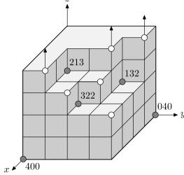
Figure 2. An example of staircase diagram.

The staircase diagram will help us visualize the structural properties of monomial ideals. For example, Figure 2 is the staircase diagram for the monomial ideal $I=\langle x^{4},y^{4},x^{3}y^{2}z^{2},xy^{3}z^{2},x^{2}yz^{3}\rangle$. In this figure the gray points are in 1-1 correspondence with the minimal generators, while the white points are in 1-1 correspondence with the irreducible components of $I$. Geometrically, $\mbox{B}(I)$ is exactly the set of interior integral points of the solid.

5. Recursive Algorithm

For bivariate monomial ideals, irreducible decomposition is simple [15]. Suppose

$$\mbox{Min}(I)=\left\{x^{a_{1}},x^{a_{2}}y^{b_{2}},\ldots,x^{a_{p-1}}y^{b_{p-1}},y^{b_{p}}\right\}$$

where $a_{1}>\cdots>a_{p-1}>0$, $0<b_{2}<\cdots<b_{p}$, and $a_{1}$ or $b_{p}$ can be infinity. Then the irreducible decomposition of $I$ is

$$I=\langle x^{a_{1}},y^{b_{2}}\rangle\cap\langle x^{a_{2}},y^{b_{3}}\rangle\cap\cdots\cap\langle x^{a_{p-2}},y^{b_{p-1}}\rangle\cap\langle x^{a_{p-1}},y^{b_{p}}\rangle.$$

Our recursive algorithm is a generalization of the above observation to higher dimensions. Let $I\subset\mathbb{K}[x_{1},\ldots,x_{n}]$ be a monomial ideal. Suppose all the distinct degrees of $x_{n}$ in $\mbox{Min}(I)$ are

$$0=d_{0}<d_{1}<\ldots<d_{s}.$$

For example, in $I=\langle x^{2}y^{3}\rangle=\langle x^{\infty},x^{2}y^{3},y^{\infty}\rangle$, the distinct degrees in $y$ are $d_{0}=0,d_{1}=3$ and $d_{3}=\infty$. We collect the coefficients of $m\in\mbox{Min}(I)$ as polynomials in $x_{n}$. Precisely, for $0\leq k\leq s$, let

$$I_{k}=\langle\mbox{Coeff}_{x_{n}}(m):\ m\in\mbox{Min}(I)\textrm{ and }\deg_{x_{n}}m\leq d_{k}\rangle\subseteq\mathbb{K}[x_{1},\ldots,x_{n-1}].$$

Then

$$I_{0}\subsetneq I_{1}\subsetneq\cdots\subsetneq I_{s}.$$ (2)

By (2), it follows that

$$B(I_{0})\supsetneq B(I_{1})\supsetneq\cdots\supsetneq B(I_{s}).$$

For the example with $I=\langle x^{\infty},x^{2}y^{3},y^{\infty}\rangle$, $I_{0}=\langle x^{\infty}\rangle=\{0\}$, $I_{1}=\langle x^{\infty},x^{2}\rangle=\langle x^{2}\rangle$, and $I_{2}=\langle x^{\infty},x^{2},1\rangle=\langle 1\rangle=\mathbb{K}[x]$.

We show how to read off the irreducible components of $I$ from those of $I_{k}$’s, which have one less variables. For any vector $\mu=(u_{1},\ldots,u_{n-1})\in\mathbb{N}^{n-1}$ and $d\in\mathbb{N}$, define

$$(\mu,d)=(u_{1},\ldots,u_{n-1},d)\in\mathbb{N}^{n}.$$

Lemma 3.

For any $\mu\in\mathbb{N}^{n-1}$ and $d\in\mathbb{N}$, $(\mu,d)\in B(I)$ if and only if there exists $k$, where $1\leq k\leq s$, such that $d_{k-1}\leq d<d_{k}$ and $\mu\in B(I_{k-1})$.

Proof.

$(\mu,d)\in B(I)$ if and only if there is no $m\in\mbox{Min}(I)$ such that $m|X^{(\mu,d)}$. As $d_{k-1}\leq d<d_{k}$, we only need to see that there is no $m\in\mbox{Min}(I)$ with $\deg_{x_{n}}m\leq d_{k-1}$. But this is equivalent to requiring that $\mu\in B(I_{k-1})$. ∎

For a set of vectors $U$ and an integer $d$, define

$$U\otimes d=\{(u,d):u\in U\}.$$

Theorem 4.

$\mbox{Irr}(I)=\bigcup_{k=1}^{s}\big{(}\mbox{Irr}(I_{k-1})\setminus\mbox{Irr}(I_{k})\big{)}\otimes d_{k}$, which is a disjoint union.

Proof.

Assume $\mu\in\mbox{Irr}(I_{k-1})\setminus\mbox{Irr}(I_{k})$. We first show that $(\mu,d_{k})\ominus 1\in B(I)$ and $\mu\ominus 1\in B(I_{k-1})\setminus B(I_{k})$. Since $\mu\in\mbox{Irr}(I_{k-1})$, we have $\mu\ominus 1\in B(I_{k-1})$, so $(\mu,d_{k})\ominus 1=(\mu\ominus 1,d_{k}-1)\in\mbox{B}(I)$ by Lemma 3. Also, by Lemma 2, there is no $\gamma\in B(I_{k-1})$ such that $\gamma>\mu\ominus 1$, in particular no $\gamma\in B(I_{k})$ such that $\gamma>\mu\ominus 1$, as $B(I_{k})\subset B(I_{k-1})$. Thus $\mu\ominus 1\notin B(I_{k})$, otherwise we would have $\mu\in\mbox{Irr}(I_{k})$ which contradicts the assumption on $\mu$.

For $(\mu,d_{k})\in\mbox{Irr}(I)$, we need to prove that $(\mu,d_{k})\ominus 1$ is maximal in $B(I)$. Assume otherwise, say $(\gamma,d)\in B(I)$ and $(\gamma,d)>(\mu,d_{k})\ominus 1$. Then $d\geq d_{k}$ or $d=d_{k}-1$. If $d\geq d_{k}$, then $\gamma\in B(I_{j})$ where $k\leq j\leq s$ by Lemma 3. Since $\gamma\geq\mu\ominus 1$ and $B(I_{k})$ is a $\delta$-set, $\gamma\in B(I_{j})$ implies $\mu\ominus 1\in B(I_{j})\subset B(I_{k})$ too, a contradiction. If $d=d_{k}-1$, then $\gamma>\mu\ominus 1$. Note that $(\gamma,d_{k}-1)\in B(I)$ implies $\gamma\in B(I_{k-1})$ by Lemma 3. However, $\mu\in\mbox{Irr}(I_{k-1})$ so there is no $\gamma\in B(I_{k-1})$ such that $\gamma>\mu\ominus 1$, a contradiction. Hence such $(\gamma,d)$ does not exist. Consequently, $(\mu,d_{k})\in\mbox{Irr}(I)$.

Conversely, assume $(\mu,d)\in\mbox{Irr}(I)$, we need to prove that there exist some $1\leq k\leq s$ such that $d=d_{k}$ and $\mu\in\mbox{Irr}(I_{k-1})\setminus\mbox{Irr}(I_{k})$. By Lemma 2, $(\mu,d)\in\mbox{Irr}(I)$ implies

$$(\mu,d)\ominus 1\in B(I),$$ (3)

and there is no $(\gamma,l)\in B(I)$ such that

$$(\gamma,l)>(\mu,d)\ominus 1.$$ (4)

By Lemma 3, (3) implies there exists $k$ such that $\mu\ominus 1\in B(I_{k-1})$, and

$$d_{k-1}\leq d-1<d_{k}.$$ (5)

By Lemma 3 again, $(\mu\ominus 1,d_{k}-1)\in\mbox{B}(I)$. Then (4) and (5) imply that $d=d_{k}$. (4) and (5) also imply that there is no $\gamma$ such that $\gamma\in B(I_{k-1})$ and $\gamma>\mu\ominus 1$, so $\mu\in\mbox{Irr}(I_{k-1})$.

It remains to prove $\mu\notin\mbox{Irr}(I_{k})$. Assume $\mu\in\mbox{Irr}(I_{k})$. Then $\mu\ominus 1\in B(I_{k})$. By Lemma 3, $(\mu\ominus 1,d_{k})\in\mbox{B}(I)$ and $(\mu\ominus 1,d_{k})>(\mu,d_{k})\ominus 1$, contradicting to $(\mu,d_{k})\in\mbox{Irr}(I)$. Thus $\mu\in\mbox{Irr}(I_{k-1})\setminus\mbox{Irr}(I_{k})$. ∎

Theorem 4 gives us the following recursive algorithm for finding irreducible decomposition of monomial ideals. Suppose we are given $I=\langle X^{\alpha_{1}},\ldots,X^{\alpha_{p}}\rangle$ and fixed variable order $x_{1}<\cdots<x_{n}$. We encode the set $\{\alpha_{1},\ldots,\alpha_{p}\}$ as a tree $\mathcal{T}$ of height $n$. Our algorithm $\mbox{Irr}(\mathcal{T})$ takes $\mathcal{T}$ as input and produce $\mbox{Irr}(I)$ as output. That is, $\mbox{Irr}(I)=\mbox{Irr}(\mathcal{T})$.

Recursive Algorithm: $\mbox{Irr}(\mathcal{T})$

Input:	$\mathcal{T}$, a tree encoding $\mbox{Min}(I)$
Output:	$S$, a set (or a tree) representing $\mbox{Irr}(I)$
Step 1.	Start at the root of $\mathcal{T}$. If the height of $\mathcal{T}$ is $1$, then $\mathcal{T}$ consists of a few leaves;
	let $d$ be the largest label on these leaves and let $S:=\{d\}$.
	Return $S$ (and stop the algorithm).
Step 2.	Now assume $\mathcal{T}$ has height at least two. Set $S:=\{\ \}$.
Step 3.	Suppose $d_{0}<d_{1}<\cdots<d_{s}$ are the labels of the children under the root of $\mathcal{T}$,
	and let $\mathcal{T}_{k}$ be the subtree extending from $d_{k}$, $0\leq k\leq s$.
	Note that the root of $\mathcal{T}_{k}$ is the node labeled by $d_{k}$, but now unlabeled.
	Find $V_{0}:=\mbox{Irr}(\mathcal{T}_{0})$ by recursive call of this algorithm.
	For $k$ from 1 to $s$ do
		3.1.	Find $\mathcal{T}_{k}:=\mbox{MinMerge}(\mathcal{T}_{k-1},\mathcal{T}_{k})$, and delete $\mathcal{T}_{k-1}$.
		3.2.	Find $V_{k}:=\mbox{Irr}(\mathcal{T}_{k})$ by recursive call of this algorithm.
		3.3.	Find $V:=V_{k-1}\setminus V_{k}$, delete $V_{k-1}$, and $S:=\mbox{Merge}(S,V\otimes d_{k})$.
Step 4.	Return ($S$).

Example 5.

We end this section by demonstrating how the algorithm is used to decompose the ideal $I=\langle x^{4},y^{4},x^{3}y^{2}z^{2},xy^{3}z^{2},x^{2}yz^{3}\rangle.$ First represent the monomials as a tree with variable order $x<y<z$, where $\mathcal{T}_{k}$’s are the subtrees extending from the node with label $d_{k}$, $k=0,1,2,3$.

Figure 3. Tree representation.

Figure 4. MinMerge step.

Figure 5. Shifting step.

Figure 4-5 show the process of finding the irredundant irreducible decomposition of $I$. For each $\mathcal{T}_{k}$, inductively MinMerge the subtrees from left to right, corresponding to Step 3.1 in the Recursive algorithm. See Figure 4. In Figure 5 we call the procedure $\mbox{Irr}(\ )$ for each $\mathcal{T}_{k}$ to compute $\mbox{Irr}(\mathcal{T}_{k})$, corresponding to Step 3.2. Since the height of $\mathcal{T}_{k}$ is 2, we bind each leaf that is not in the most-right side of $\mathcal{T}_{k}$ with the node of height 2 on the next path - just do the shifting in adjacent paths, see Figure 5. Finally we find the paths in $\mbox{Irr}(\mathcal{T}_{k-1})$ that are not in $\mbox{Irr}(\mathcal{T}_{k})$. The one with a mark $\times$ in $\mbox{Irr}(\mathcal{T}_{k})$ is discarded. Then bind the resulting paths with $d_{k}$. The irreducible components can be read from the last figure:

$$\mbox{Irr}(I)=\{(4,4,2),(4,2,3),(3,3,3),(4,1,\infty),(2,3,\infty),(1,4,\infty)\}.$$

6. Incremental Algorithm

In this section we shall present an incremental algorithm based on the idea of adding one generator at a time. This algorithm can be viewed as an improvement of Alexander Dual method ([14, 17]). We maintain an output list of irreducible components, and at each step we use a new generator to update the output list. In [17], it is not clear how to select good candidates that need to be updated, and the updating process there is also inefficient. Our algorithm avoids these two deficiencies. We establish some rules that help us to exclude many unnecessary comparisons.

Monomial ideal are much simpler than general ideals. The next theorem tells us that monomial ideals satisfy distribution rules for the operations “$+$” and “$\cap$”. These rules may not be true for general ideals.

Theorem 6 (Distribution Rules).

Let $I_{1},\ldots,I_{t},J$ be any monomial ideals in $\mathbb{K}[X]$. Then

1. $(I_{1}+\ldots+I_{t})\cap J=I_{1}\cap J+\ldots+I_{t}\cap J$, and

2. $(I_{1}\cap\ldots\cap I_{t})+J=(I_{1}+J)\cap\ldots\cap(I_{t}+J)$.

Proof.

By induction, we just need to prove the case for $t=2$. Note that (b) follows form (a), as

$$(I_{1}+J)\cap(I_{2}+J) = I_{1}\cap(I_{2}+J)+J\cap(I_{2}+J)$$

$$= I_{1}\cap I_{2}+I_{1}\cap J+J\cap I_{2}+J$$

$$= I_{1}\cap I_{2}+J.$$

To prove (a) for the case $t=2$, suppose $h$ is a generator for $(I_{1}+I_{2})\cap J$. Then $h$ must be in $(I_{1}+I_{2})$ and $J$. Since $(I_{1}+I_{2})\cap J$ is also a monomial ideal, $h$ is a monomial. The fact that $h\in I_{1}+I_{2}$ implies that $h$ is in either $I_{1}$ or $I_{2}$. Hence $h$ is in $I_{1}\cap J$ or in $I_{2}\cap J$, so $h\in I_{1}\cap J+I_{2}\cap J$. Going backward yields the proof for the other direction. ∎

Theorem 6 gives us an incremental algorithm for irreducible decomposition of monomial ideals. Precisely, we have the following situation at each incremental step: Given the irreducible decomposition $\mbox{Irr}(I)$ of an arbitrary ideal $I$ and a new monomial $X^{\alpha}$ where $\alpha=(a_{1},\ldots,a_{n})\in\mathbb{N}^{n}$, we want to decompose $\widetilde{I}=I+\langle X^{\alpha}\rangle$. By the distribution rule (b),

$$\widetilde{I}=\left(\bigcap_{\beta\in\mbox{Irr}(I)}m^{\beta}\right)+\langle X^{\alpha}\rangle=\bigcap_{\beta\in\mbox{Irr}(I)}\left(m^{\beta}+\langle X^{\alpha}\rangle\right).$$ (6)

We need to see how to decompose each ideal on the right hand side of (6) and how to get rid of redundant components. We partition $\mbox{Irr}(I)$ into two disjoint sets:

$$T_{1}^{\alpha} = \{\beta\in\mbox{Irr}(I):\alpha\nprec\beta\},\textrm{ and}$$ (7)

$$T_{2}^{\alpha} = \{\beta\in\mbox{Irr}(I):\alpha\prec\beta\}.$$ (8)

Note that if $X^{\alpha}\in I$ then $T_{2}^{\alpha}=\phi$. For each $\beta\in T_{1}^{\alpha}$, we have $X^{\alpha}\in m^{\beta}$, thus

$$m^{\beta}+\langle X^{\alpha}\rangle=m^{\beta}.$$ (9)

For each $\beta\in T_{2}^{\alpha}$, we have $X^{\alpha}\notin m^{\beta}$. In this case, we split $\langle X^{\alpha}\rangle$ as

$$\langle X^{\alpha}\rangle=\bigcap_{j=1}^{n}\langle x_{j}^{a_{j}}\rangle.$$

By the distribution rule (b), we have

$$m^{\beta}+\langle X^{\alpha}\rangle=\bigcap_{j=1}^{n}\left(m^{\beta}+\langle x_{j}^{a_{j}}\rangle\right).$$

Define

$$\beta^{(\alpha,j)}=(b_{1},\ldots,b_{j-1},a_{j},b_{j+1},\ldots,b_{n}),\quad 1\leq j\leq n.$$

Since $\alpha\prec\beta$, we have $a_{j}<b_{j}$ for all $1\leq j\leq n$. Hence $m^{\beta}+\langle x_{j}^{a_{j}}\rangle=m^{\beta^{(\alpha,j)}}$, and

$$m^{\beta}+\langle X^{\alpha}\rangle=\bigcap_{j=1}^{n}m^{\beta^{(\alpha,j)}}.$$ (10)

Therefore,

$$\mbox{Irr}(\widetilde{I})=\mbox{MaxMerge}\left(T_{1}^{\alpha},\{\beta^{(\alpha,j)}:\beta\in T_{2}^{\alpha}\textrm{ and }1\leq j\leq n\}\right).$$ (11)

It remains to see which of the components in the right hand side of the above expression belong to $\mbox{Irr}(\widetilde{I})$, so others are redundant.

Lemma 7.

$T_{1}^{\alpha}\subset\mbox{Irr}(\widetilde{I})$.

Proof.

Let $\beta_{1}\in T_{1}^{\alpha}$. By equation (11) if $\beta_{1}\notin\mbox{Irr}(\widetilde{I})$, then there exists some $\beta_{2}\in T_{2}^{\alpha}$ such that $\beta_{1}$ is maxmergeed by $\beta_{2}^{(\alpha,j)}$ for some $j$, ie. $\beta_{1}\leq\beta_{2}^{(\alpha,j)}$. Since $\beta_{2}^{(\alpha,j)}<\beta_{2}$, $\beta_{1}\leq\beta_{2}^{(\alpha,j)}$ implies that $\beta_{1}<\beta_{2}$, which contradicts with the fact that $\beta_{1},\beta_{2}\in\mbox{Irr}(I)$. Hence $\beta_{1}\in\mbox{Irr}(\widetilde{I})$ as claimed. ∎

Lemma 7 shows that the elements in $T_{1}^{\alpha}$ will be automatically in $\mbox{Irr}(\widetilde{I})$. Now we turn to the components $\beta^{(\alpha,j)}$. For $\beta\in T_{2}^{\alpha}$, define

$$M_{\beta}=\{m\in\mbox{Min}(I):m|X^{\beta}\}.$$ (12)

For $m\in M_{\beta}$, if $\deg_{x_{u}}m=b_{u}$, then we say $m$ matches $\beta$ in $x_{u}$. It is possible that one monomial matches $\beta$ in multiple variables. For example, with $I=\langle x^{2},y^{2},z^{2},xy,xz,yz\rangle$ and $\beta=(1,1,2)\in\mbox{Irr}(I)$, the monomial $xy$ matches $\beta$ in $x$ and $y$. We say $m$ matches $\beta$ only in $x_{u}$ if $\deg_{x_{u}}m=b_{u}$ and $\deg_{x_{k}}m<b_{k}$ for all $k\neq u$.

Lemma 8.

For each $\beta=(b_{1},\ldots,b_{n})\in T_{2}^{\alpha}$ and each $1\leq u\leq n$, there exists $m\in M_{\beta}$ such that $m$ matches $\beta$ only in $x_{u}$.

Proof.

Note that a vector $\gamma\in\mbox{B}(I)$ is maximal if and only if $X^{\gamma}\cdot x_{u}\in I$ for every $u$. Since $\beta\in\mbox{Irr}(I)$, $\beta\ominus 1$ is maximal in $B(I)$. Thus, for each $1\leq u\leq n$, $X^{\beta\ominus 1}\cdot x_{u}\in I$, so there exists a monomial say $m\in\mbox{Min}(I)$ such that $m|X^{\beta\ominus 1}\cdot x_{u}$. Then $\deg_{x_{k}}m<b_{k}$ for $k\neq u$. If $\deg_{x_{u}}m<b_{u}$ as well, then $m|X^{\beta\ominus 1}$, which implies that $X^{\beta\ominus 1}\in I$, a contradiction. Therefore $\deg_{x_{u}}m=b_{u}$. Note that $X^{\beta\ominus 1}\cdot x_{u}|X^{\beta}$, so $m\in M_{\beta}$. ∎

For any set of monomials $A\subset\mathbb{K}[X]$, define $\textbf{max}(A)$ be the exponent $\gamma$ such that $X^{\gamma}=\mbox{Lcm}(A)$.

Lemma 9.

$\max(M_{\beta})=\beta$.

Proof.

By the definition of $M_{\beta}$, we know that $\max(M_{\beta})\leq\beta$. By Lemma 8 we have $\max(M_{\beta})\geq\beta$. Thus $\max(M_{\beta})=\beta$. ∎

For $k\neq u$, let

$$d(\beta,u,k)=\min\{\deg_{x_{u}}m:m\in M_{\beta}\text{ matching $\beta$ only in $x_{k}$}\}.$$ (13)

Note that $d(\beta,u,k)<b_{u}$. Define

$$d(\beta,u)=\max_{1\leq k\leq n,k\neq u}\{d(\beta,u,k)\}.$$

Lemma 10.

For each $\beta\in T_{2}^{\alpha}$ and $1\leq u\leq n$, $\beta^{(\alpha,u)}\in\mbox{Irr}(\widetilde{I})$ if and only if $d(\beta,u)<a_{u}$.

Proof.

Suppose $d(\beta,u)<a_{u}$. We want to prove that $\beta^{(\alpha,u)}\in\mbox{Irr}(\widetilde{I})$. By Lemma 2, this is equivalent to proving that $\beta^{(\alpha,u)}\ominus 1\in\mbox{B}(\widetilde{I})$ and is maximal. Assume $\beta^{(\alpha,u)}\ominus 1\notin\mbox{B}(\widetilde{I})$. Then there exists $m\in\mbox{Min}(I)\cup\{X^{\alpha}\}$ such that $m|X^{\beta^{(\alpha,u)}\ominus 1}$. First note that $m\neq X^{\alpha}$ because $X^{\alpha}$ can not divide $X^{\beta^{(\alpha,u)}\ominus 1}$. Thus $m\in\mbox{Min}(I)$, which implies $X^{\beta^{(\alpha,u)}\ominus 1}\in I$. Since $\beta^{(\alpha,u)}\ominus 1<\beta\ominus 1$, we have $X^{\beta\ominus 1}\in I$, contradicting to $\beta\in\mbox{Irr}(I)$. Hence $\beta^{(\alpha,u)}\ominus 1\in\mbox{B}(\widetilde{I})$. We next need to prove that $\beta^{(\alpha,u)}\ominus 1$ is maximal in $\mbox{B}(\widetilde{I})$, that is, $X^{\beta^{(\alpha,u)}\ominus 1}\cdot x_{k}\in\widetilde{I}$ for every $k$. In the case for $k=u$, we have $X^{\alpha}|X^{\beta^{(\alpha,u)}\ominus 1}\cdot x_{u}$. For any $k\neq u$, let $m$ be any monomial in (13) such that $\deg_{x_{u}}m=d(\beta,u,k)$. Then $\deg_{x_{u}}m=d(\beta,u,k)\leq d(\beta,u)<a_{u}$, hence $m|X^{\beta^{(\alpha,u)}\ominus 1}\cdot x_{k}$ as $\deg_{x_{k}}m=b_{k}$ and $\deg_{x_{j}}m\leq b_{j}-1$ for $j\neq u,k$.

Conversely, suppose $\beta^{(\alpha,u)}\in\mbox{Irr}(\widetilde{I})$. We want to prove that $d(\beta,u)<a_{u}$. We know that $\beta^{(\alpha,u)}\ominus 1$ is maximal in $\mbox{B}(\widetilde{I})$. Thus $X^{\beta^{(\alpha,u)}\ominus 1}\cdot x_{k}\in\widetilde{I}$ for every $k$. For any $k\neq u$, suppose $X^{\beta^{(\alpha,u)}\ominus 1}\cdot x_{k}$ is divisible by $m\in\mbox{Min}(I)\cup\{X^{\alpha}\}$. Then

$$\deg_{x_{u}}m\leq a_{u}-1<b_{u},\quad\deg_{x_{j}}m\leq b_{j}-1,\ j\neq u,k,$$ (14)

and $\deg_{x_{k}}m\leq b_{k}$. As $X^{\beta^{(\alpha,u)}\ominus 1}\in\mbox{B}(\widetilde{I})\subset\mbox{B}(I)$, $m$ can not divide $X^{\beta^{(\alpha,u)}\ominus 1}$. Hence $\deg_{x_{k}}m\leq b_{k}$. So $m$ matches $\beta$ only in $x_{k}$. Note that $m\neq X^{\alpha}$, so $m\in M$ and thus $m\in M_{\beta}$. It follows that $d(\beta,u,k)\leq a_{u}-1$ by (14). Therefore, $d(\beta,u)<a_{u}$ as desired. ∎

By the above lemma, for each $\beta\in T_{2}^{\alpha}$, we only need to find $M_{\beta}$ and $d(\beta,u)$, which will tell us whether $\beta^{(\alpha,u)}\in\mbox{Irr}(\widetilde{I})$. This gives us the following incremental algorithm.

Incremental algorithm

Input:	$M$, a set of monomials in $n$ variables $x_{1},\ldots,x_{n}$.
Output:	$\mbox{Irr}(I)$, the irredundant irreducible components of the ideal $I$ generated by $M$.
Step 1.	Compute $\mbox{MinMerge}(M)$ and sort it into the form:
				$\mbox{MinMerge}(M)=\{x_{1}^{c_{1}},\ldots,x_{n}^{c_{n}},X^{\alpha_{1}},\ldots,X^{\alpha_{p}}\},$
	where $c_{i}$ can be $\infty$ and $\{X^{\alpha_{1}},\ldots,X^{\alpha_{p}}\}$ are sorted in lex order with variable
	order $x_{1}<\ldots<x_{n}$. Set
				$T:=\{(a_{1},\ldots,a_{n})\}$.
Step 2.	For each $k$ from 1 to $p$ do:
		2.1. Set the temporal variables $V=\emptyset$ and $\alpha:=\alpha_{k}$.
		2.2. For every $\beta\in T$ with $\alpha\nprec\beta$ do
				$V:=V\cup\{\beta\}.$
		2.3. For every $\beta\in T$ with $\alpha\prec\beta$ do,
			$\bullet$ find $M_{\beta}$ as defined in (12);
			$\bullet$ for $1\leq u\leq n$, compute $d(\beta,u)$, and if $d(\beta,u)<a_{u}$ then update
				$V:=V\cup\{\beta^{(\alpha,u)}\}.$
		2.4. Set $T:=V$.
Step 3.	Output $T$.

We next prove that there is a nice property of the above algorithm for generic monomial ideals, that is, the size of $T$ is always non-decreasing at each stage when a new generator is added. This will allow us to bound the running time of the algorithm in term of input and output sizes.

Theorem 11.

Suppose $I$ is generic and $\mbox{Min}(I)=\{x_{1}^{c_{1}},\ldots,x_{n}^{c_{n}},X^{\alpha_{1}},\ldots,X^{\alpha_{p}}\}$ where $X^{\alpha_{k}}$’s are sorted in lex order with variable order $x_{1}<\ldots<x_{n}$. Let $\widehat{I}=\langle x_{1}^{c_{1}},\ldots,x_{n}^{c_{n}},$ $X^{\alpha_{1}},$$\ldots,X^{\alpha_{p-1}}\rangle$. Then $|\mbox{Irr}(\widehat{I})|\leq|\mbox{Irr}(I)|$.

Proof.

Keep notations as above. For every $\beta\in T_{2}^{\alpha}$, $b_{n}=c_{n}$. Thus $x_{n}^{c_{n}}$ is the only monomial in $M_{\beta}$ that has degree in $x_{n}$ larger than $a_{n}$. Hence $d(\beta,n)<a_{n}$ and $\beta^{(\alpha,n)}\in\mbox{Irr}(I)$. By the equation (11) and Lemma 7,

$$|\mbox{Irr}(I)|\geq|T_{1}^{\alpha}|+|\{\beta^{(\alpha,n)}:\beta\in T_{2}^{\alpha}\}|=|T_{1}^{\alpha}|+|T_{2}^{\alpha}|=|\mbox{Irr}(\widehat{I})|.\qed$$

The reader might wonder whether a similar statement holds in non-generic case as well. The answer is negative. Let $I=\langle x^{3},y^{3},z^{2},w^{2},x^{2}yz,xy^{2}w\rangle\subset\mathbb{K}[x,y,z,w]$ with lex order and $x<y<z<w$. Then

$$\mbox{Irr}(I)=\{(3,3,1,1),(2,3,2,1),(3,2,1,2),(3,1,2,2),(2,2,2,2),(1,3,2,2)\}.$$

By adding $X^{\alpha}=xyzw$, we can see $\beta=(2,2,2,2)\in T_{2}^{\alpha}$. Note that $M_{\beta}=\{x^{2}yz,xy^{2}w,z^{2},$ $w^{2}\}$. Since $d(\beta,u)=1=a_{u}$ for $u=1,2,3,4$, no new $\beta^{(\alpha,j)}$ will be generated. Thus the number of irreducible components decreases by 1 instead.

We find the irreducible components for the monomial ideal in Example 5 again by the flow of our incremental algorithm.

Example 12.

Decompose

$$I=\langle x^{4},y^{4},x^{3}y^{2}z^{2},xy^{3}z^{2},x^{2}yz^{3}\rangle.$$

Note: “$\checkmark$” means $\beta^{(\alpha,u)}\in\mbox{Irr}(\widetilde{I})$ for corresponding $\beta,\alpha$ and $u$, while “$\times$” means not.

Step 1.	$M=\{x^{4},y^{4},z^{\infty},x^{3}y^{2}z^{2},xy^{3}z^{2},x^{2}yz^{3}\}$. Set $T:=\{(4,4,\infty)\}.$
Step 2.	(i) For $\alpha=(3,2,2)$ do:
		2.1. $V:=\phi$.
		2.2. Since $\alpha\prec(4,4,\infty)$, $V:=\phi$.
		2.3. Let $\beta=(4,4,\infty)$. We find $M_{\beta}=\{x^{4},y^{4}\}$.
			So we have $d\{\beta,1\}=0$($\checkmark$), $d\{\beta,2\}=0$($\checkmark$) and $d\{\beta,3\}=0$($\checkmark$).
			Then $V:=\{(3,4,\infty),(4,2,\infty),(4,4,2)\}.$
		2.4. Let $T:=V$.
	(ii) For $\alpha=(1,3,2)$ do:
		2.1. $V:=\phi$.
		2.2. Update $V$ by $V:=\{(4,4,2),(4,2,\infty)\}$.
		2.3. $\alpha\prec(3,4,\infty)$.
			Let $\beta=(3,4,\infty)$. We find $M_{\beta}=\{y^{4},x^{3}y^{2}z^{2}\}$.
			So $d\{\beta,1\}=0$($\checkmark$), $d\{\beta,2\}=2$($\checkmark$) and $d\{\beta,3\}=2$($\times$).
			Then $V:=\{(4,4,2),(4,2,\infty),(1,4,\infty),(3,3,\infty)\}.$
		2.4. Let $T:=V$.
	(iii) For $\alpha=(2,1,3)$ do:
		2.1. $V:=\phi$.
		2.2. $V:=\{(4,4,2),(1,4,\infty)\}$.
		2.3. $\alpha\prec(4,2,\infty)$, and $\alpha\prec(3,3,\infty)$.
			$\bullet$ Let $\beta=(4,2,\infty)$. We find $M_{\beta}=\{x^{4},x^{3}y^{2}z^{2}\}$.
				So $d\{\beta,1\}=3$($\times$), $d\{\beta,2\}=0$($\checkmark$) and $d\{\beta,3\}=2$($\checkmark$).
				Then $V:=\{(4,4,2),(1,4,\infty),(4,1,\infty),(4,2,3)\}.$
			$\bullet$ Let $\beta=(3,3,\infty)$. Then $M_{\beta}=\{x^{3}y^{2}z^{2},xy^{3}z^{2}\}$.
				$d\{\beta,1\}=1$($\checkmark$), $d\{\beta,2\}=2$($\times$), $d\{\beta,3\}=2$($\checkmark$).
				So $V:=\{(4,4,2),(1,4,\infty),(4,1,\infty),(4,2,3),(2,3,\infty),(3,3,3)\}.$
		2.4. Let $T:=V$.
Step 3.	Output $T$				$=\{(4,4,2),(1,4,\infty),(4,1,\infty),(4,2,3),(2,3,\infty),(3,3,3)\}$
					$=\{(4,4,2),(4,2,3),(3,3,3),(4,1,\infty),(2,3,\infty),(1,4,\infty)\}$.

Some preprocess can be taken right before Step 2 to improve the efficiency of the incremental algorithm. For each $u\in\{1,\ldots,n\}$, we partition $M$ into disjoint subsets such that the monomials in each subset have the same degree in $x_{u}$. We then store these information, which requires memory complexity $O(n\cdot p)$. For each $\beta\in T_{2}^{\alpha}$, we can find $M_{\beta}$ by only checking the monomials in the subset with degree $b_{u}$ in variable $x_{u}$ for every $u$. Note that for generic monomial ideals each subset contains a unique monomial. In this case $M_{\beta}$ contains $n$ monomials, and it can be found by $O(n)$ operations, instead of $O(p)$ operations by scanning through the whole input monomial set.

7. Time Complexity and Conclusion

We estimate the running time of our algorithms by counting the number of monomial operations (ie. comparisons and divisibility) used. Our recursive algorithm depends heavily on the number of distinct degrees of each variable. Let $s_{j}$ be the number of distinct degrees of $x_{j}$ where $j=1,\ldots,n$. Then the total number of merge of subtrees used by the algorithm is at most $\prod_{j=1}^{n}s_{j}$. Since each subtree has at most $p$ leaves(ie. $p$ generators), each merge takes $O(p^{2})$ monomial operations. Hence the algorithm uses $O(p^{2}\cdot\prod_{j=1}^{n}s_{j})$ monomial operations. This algorithm is more efficient for highly non-generic monomial ideals. The benchmark analysis in [20] compare several algorithms based on various slicing strategies, including our recursive algorithm. It is shown there that our algorithm performs as a very close second best one.

The running time of our incremental algorithm is harder to estimate for general ideals. For generic ideals, however, we can bound the time in terms of input and output sizes. More precisely, suppose

$$I=\langle x_{1}^{c_{1}},\ldots,x_{n}^{c_{n}},X^{\alpha_{1}},\ldots,X^{\alpha_{p}}\rangle$$

is a generic monomial ideal in $\mathbb{K}[X]$ where $X^{\alpha_{k}}$’s are sorted in lex order with variable order $x_{1}<\ldots<x_{n}$. For $0\leq k\leq p$, let

$$I_{(k)}=\langle x_{1}^{c_{1}},\ldots,x_{n}^{c_{n}},X^{\alpha_{1}},\ldots,X^{\alpha_{k}}\rangle.$$

All these ideals are generic. By Theorem 11, we have

$$1=|\mbox{Irr}(I_{(0)})|\leq|\mbox{Irr}(I_{(1)})|\leq\cdots\leq|\mbox{Irr}(I_{(p)})|=|\mbox{Irr}(I)|.$$

In an arbitrary stage of the incremental algorithm, we try to find the irreducible components of $I_{(k)}$ from those of $I_{(k-1)}$. For each $\beta\in\mbox{Irr}(I_{(k-1)})$, only those $\beta$ in $T_{2}^{\alpha_{k}}$ (as defined in (8)) need to be updated. Note that $I$ is generic, by the preprocess $M_{\beta}$ can be found in $O(n)$ operations. The numbers $d(\beta,u,k)$, $1\leq u\neq k\leq n$, can be computed by scanning through the monomials in $M_{\beta}$ once, thus using only $O(n)$ monomial operations. Then the numbers $d(\beta,u)$, $1\leq u\leq n$, can be computed in $O(n^{2})$ operations. Hence for each $\beta\in T_{2}^{\alpha_{k}}$, Step 2.3 uses at most $O(n+n^{2})=O(n^{2})$ monomial operations. Since $T\supset T_{2}^{\alpha_{k}}$ has at most $\ell$ elements where $\ell=|\mbox{Irr}(I)|$, Step 2.3 needs at most $O(n^{2}\ell)$ monomial operations. Therefore, the total number of monomial operations is at most $O(n^{2}p\ell)$. In fact, $T_{2}^{\alpha_{k}}$ is usually a small subset of $T$, the actual running time is much better than our worst-case estimate indicates.

We also want to point out that for generic monomial ideals, the incremental algorithm is an improved version of the recursive algorithm. Suppose we add the new monomial $X^{\alpha_{k}}$ into $I_{(k-1)}$. In Step 3.2 of the recursive algorithm, we need to compute $\mbox{Irr}(\mathcal{T}_{k})$. But in Step 2.3 of the incremental algorithm, only $\beta\in T_{2}^{\alpha_{k}}$ need to be updated. We have the observation that $T_{2}^{\alpha_{k}}$ is a small subset of $\mbox{Irr}(\mathcal{T}_{k})\otimes c_{n}$. By this observation we conclude the incremental algorithm is more efficient than the recursive algorithm for generic monomial ideals. In non-generic case, the comparison is not clear.

In all previous algorithms (including our recursive one) for monomial decomposition, the storage in the intermediate stages may grow exponentially larger than the output size. Our incremental algorithm seems to be the first algorithm for monomial decomposition that the intermediate storage is bounded by the final output size. Note that the output size $\ell$ can be exponentially large in $n$. In fact, it is proven in [1] that $\ell=O(p^{[\frac{n}{2}]})$ for large $p$. Since the output size can be exponential in $n$, it is impossible to have a polynomial time algorithm for monomial decomposition.

8. Acknowledgement

We thank Alexander Milowski and Bjarke Roune for comments and suggestions, and Ezara Miller for helpful communications (especially for providing some of the diagrams).

References

- [1] Agnarsson, G., 1997. The number of outside corners of monomial ideals. J Pure Appl Algebra. 117&118, 3-22.
- [2] Anwar, I., 2007. Janet’s Algorithm. Eprint arXiv, 0712.0068.
- [3] Block, F., Yu, J., 2006. Tropical convexity via cellular resolutions. J Algebr Comb. 24(1), 103-114. Eprint arXiv,math/0503279.
- [4] Bayer,D., Peeva, I., Sturmfels, B., 1998, Monomial resolutions. Math Res Lett. 5(5),31-46.
- [5] Cox, D., Little, J., O’Shea, D., 1997. Ideals, Varieties, and Algorithms, An Introduction to Computational Algebraic Geometry and Commutative Algebra. Springer-Verlag.
- [6] Cox, D., Little, J., O’Shea, D., 1998. Using Algebraic Geometry. In: Graduate Texts in Mathematics, vol. 185. Springer.
- [7] Eisenbud, D., 1995. Commutative algebra, with a view toward algebraic geometry. In: Graduate Texts in Mathematics, vol. 150, Springer.
- [8] Far, J., Gao, S., 2006. Computing Gröbner bases for vanishing ideals of finite sets of points. Applied Algebra, Algebraic Algorithms and Error-Correcting Codes. In: Springer Lecture Notes in Computer Science, no. 3857, Springer-Verlag, 118-127.
- [9] Gao, S., Rodrigues, V., Stroomer, J., 2003. Gröbner basis structure of finite sets of points. Preprint.
- [10] Gao, S., Zhu, M., 2008. Upper bound on the number of irreducible components of monomial ideals. In preparation.
- [11] Hoşten S., Smith, G., 2002. Monomial ideals. Computations in algebraic geometry with Macaulay 2, Springer-Verlag.
- [12] Hoşten S., Sturmfels, B., 2007. Computing the integer programming gap. Combinatorica, 27, 367-382.
- [13] Jarrah, A., Laubenbacher, R., Stigler, B., Stillman, M., 2006. Reverse-engineering of polynomial dynamical systems. Adv Appl Math, 39(4), 477-489.
- [14] Miller, E., 2000. Resolutions and Duality for Monomial Ideals. PhD thesis, University of California, Berkeley, Mathematics Department.
- [15] Miller, E., Sturmfels, B., 1999. Monomial ideals and planar graphs. Applied Algebra, Algebraic Algorithms and Error-Correcting Codes. In: Springer Lecture Notes in Computer Science, no. 1719, Springer-Verlag, AAECC-13 proceedings (Honolulu, Nov. 1999), pp. 19-28.
- [16] Miller, E., Sturmfels, B., 2004. Combinatorial Commutative Algebra. In: Graduate Texts in Mathematics, vol. 227, Springer.
- [17] Milowski, A., 2004. Computing Irredundant Irreducible Decompositions of Large Scale Monomial Ideals. In: Proceedings of the International Symposium on Symbolic and Algebraic Computation 04, 235-242.
- [18] Roune, B., 2007. The label algorithm for irreducible decomposition of monomial ideals. Eprint arXiv,0705.4483.
- [19] Roune, B., 2008. Solving Thousand-Digit Frobenius Problems Using Gröbner Bases. J Symb Comput, 43(1), 1-7. Eprint arXiv,math/0702040.
- [20] Roune, B., 2008. The Slice Algorithm For Irreducible Decomposition of Monomial Ideals. To appear in J Symb Comput. Eprint arXiv,0806.3680.
- [21] Sturmfels, B., Gröebner Bases and Convex Polytopes. In: AMS University Lecture Series, vol. 8.
- [22] Sturmfels, B., Sullivant, S., 2006. Combinatorial secant varieties. Pure and Applied Mathematics Quarterly, 2, 285-309. Eprint arXiv,math/0506223.
- [23] Vasconcelos, W., 1998. Computational Methods in Commutative Algebra and Geometry. Algorithms and Computation in Mathematics, vol. 2. Springer-Verlag.
- [24] Villarreal, R., 2001. Monomial algebras. Monographs and Textbooks in Pure and Applied Mathematics, vol. 238. CRC Press.