Signatures of unstable semiclassical trajectories in tunneling

Abstract

It was found recently that processes of multidimensional tunneling are generally described at high energies by unstable semiclassical trajectories. We study two observational signatures related to the instability of trajectories. First, we find an additional power-law dependence of the tunneling probability on the semiclassical parameter as compared to the standard case of potential tunneling. The second signature is substantial widening of the probability distribution over final–state quantum numbers. These effects are studied using modified semiclassical technique which incorporates stabilization of the tunneling trajectories. The technique is derived from first principles. We obtain expressions for the inclusive and exclusive tunneling probabilities in the case of unstable semiclassical trajectories. We also investigate the “phase transition” between the cases of stable and unstable trajectories across certain “critical” value of energy. Finally, we derive the relation between the semiclassical probabilities of tunneling from the low–lying and highly excited initial states. This puts on firm ground a conjecture made previously in the semiclassical description of collision–induced tunneling in field theory.

1 Introduction

Tunneling in systems with several degrees of freedom is an exceptionally rich subject of investigation [1, 2]. The features and probability of multidimensional tunneling depend crucially on the properties of underlying system, or rather on the degree of complexity of its classical dynamics. In particular, expressions for the tunnel splittings of energy levels are qualitatively different in the cases of integrable [3, 4, 5] and near-integrable [6, 7, 8, 9] dynamics. The other drastically different case, tunneling in irregular (chaotic or mixed) systems, has been a subject of continuous theoretical [10, 11, 12, 13, 14, 15, 16, 17] and experimental [18, 19, 20, 21] research for the last few decades.

The basic concept in multidimensional tunneling is dynamical tunneling [22, 23]. It is related to the classical dynamics and reflects the fact that transitions of a multidimensional system between the in- and out- regions of phase space may be classically forbidden even if there is no energy barrier separating the regions. In this case the quantum probability ${\cal P}$ of transition is on general grounds exponentially suppressed,

$${\cal P}=A\,\mathrm{e}^{-F/\hbar}\;,$$ (1)

where $F$ and $A$ are the suppression exponent and prefactor respectively. The transition itself is called dynamical tunneling [23], since the reasons for its exponential suppression are hidden in the particularities of classical dynamics.

A new mechanism of dynamical tunneling has been independently discovered in Refs. [24, 25] and [26]. It governs tunneling in non–separable systems with multiple degrees of freedom at energies exceeding certain critical energy $E_{c}$. The value of the latter energy depends on the details of the system dynamics but is always greater than the height of the potential barrier between the in- and out- states of the process. The new mechanism is general: it is relevant for tunneling in regular [26, 27, 28] and irregular [24, 16] scattering problems, for transitions in time-dependent one–dimensional potentials [25, 29, 30], in the case of chaotic tunneling [12, 31]. Another example emerges in field theory where the new mechanism is generically inherent in the processes of collision–induced tunneling at high energies [32, 33].

The defining characteristics of the new mechanism have been given within the semiclassical approach. It was noted that the semiclassical trajectories describing tunneling transitions acquire qualitatively new properties at $E>E_{c}$. Instead of connecting directly the in- and out- regions of the process, the trajectories end up performing unstable motion on the boundary between the regions. In the simplest case of two degrees of freedom this unstable motion proceeds along the periodic orbit describing oscillations on top of the saddle point of the potential. Following Ref. [26], we call the latter orbit sphaleron (or simply unstable periodic orbit).

In general case of systems with more than two degrees of freedom the boundary between the in- and out- regions is normally hyperbolic invariant manifold (NHIM) [35]; the trajectories in the new mechanism get attracted to this manifold. In this case we use the term sphaleron in the sense equivalent to NHIM.

Due to the above property of the trajectories, tunneling at $E>E_{c}$ proceeds in two stages. First, the long-living sphaleron “state” gets created. Second, the sphaleron decays into the final asymptotic region with the probability of order one. The overall transition remains exponentially suppressed, since creation of the sphaleron costs exponentially small probability factor. We call the overall transition sphaleron–driven tunneling.

The aim of the present paper is twofold. First, we analyze the possibility of direct experimental observation of the the mechanism of sphaleron–driven tunneling. To the best of our knowledge, such observation has not been performed so far. We study two signatures of the new mechanism which may be helpful in future experiments. Second, we systematically develop modified semiclassical method for the calculation of tunneling probability in the sphaleron–driven case.

We discuss two experimental signatures of the new tunneling mechanism. In Ref. [28] we have found that the probability of sphaleron–driven tunneling contains additional power-law dependence on $\hbar$ as compared to the ordinary case of potential tunneling. The additional factor is $\hbar^{1/2}$ in the case of inclusive tunneling processes, i.e. processes without specification of the out-state. In this paper we review the result of Ref. [28] and extend the analysis to the new case of exclusive processes, i.e. processes with fixed out-state quantum numbers. We show that the additional factor is $\hbar$ in this case. For example, consider two–dimensional inclusive processes. Then, the prefactor $A$ in Eq. (1) is proportional to $\hbar^{1/2}$ and $\hbar$ in the cases of potential and sphaleron–driven tunneling respectively. For exclusive processes this dependence is $\hbar$ ($\hbar^{2}$) in the potential (sphaleron–driven) case.

It is important to stress that the dependence of the tunneling probability on $\hbar$ can, in principle, be studied experimentally. Indeed, the semiclassical parameter, which we denote by $\hbar$ for convenience, is in fact a certain dimensionless combination of the Planck constant and parameters characterizing the system. Changing the latter parameters one varies the value of effective $\hbar$.

The second manifestation of the new mechanism is spreading of the out-state of the tunneling process over an anomalously wide range of quantum numbers. This effect was originally observed in Ref. [25] in the case of a one-dimensional system with time–dependent potential; here we show that it is present in the multidimensional case, cf. Ref. [30]. Physically, the widening of the out-state is related to the fact that the intermediate sphaleron orbit is classically unstable; thus, classical trajectories describing sphaleron decay spread exponentially over phase space. In quantum case this corresponds to the final state wave function which is almost constant in some region of quantum numbers.

In the second part of this paper we develop the modified semiclassical technique which is essential in the case of sphaleron–driven tunneling. The motivation for the new technique becomes clear if we try to apply the standard method of complex trajectories to the problem of inclusive sphaleron–driven tunneling in the scattering setup. Since the overall time interval of the scattering problem is infinite, one generically finds two different trajectories corresponding to the two stages of the new tunneling mechanism: one trajectory starts in the in-region and tends to the sphaleron orbit as $t\to+\infty$, and the second trajectory starts at the sphaleron at $t\to-\infty$ and arrives into the out-region. The first of these trajectories is unstable: it can be destroyed by infinitesimally small changes in the initial Cauchy data. It is problematic to find unstable trajectories numerically. Besides, one wonders how to join the two trajectories in order to describe the overall two–stage process. Finally, it is not clear how to calculate the prefactor $A$ of the tunneling probability. Indeed, the standard formula for the prefactor deals with the linear perturbations above the tunneling trajectory. When the trajectory in question is unstable these perturbations grow exponentially with time. Then the standard formula gives $A=0$, which is obviously incorrect.

Our modified semiclassical method overcomes the above difficulties. The main idea of the method was proposed in Refs. [26, 28]; here we present its detailed derivation. The modified method is summarized as follows. We evaluate the Feynman path integral for the tunneling amplitude in two steps. First, we restrict the integral to paths which arrive into the out-region in a fixed time interval $\tau$. Second, we integrate over $\tau$. The integration at step $1$ can be done by the standard saddle-point method, since all trajectories at finite $\tau$ are stable and interpolate between the in- and out- regions. On the other hand, the ordinary integral over $\tau$ at step 2 should be evaluated with care. In particular, we find that in the case of sphaleron–driven tunneling this integral is saturated in the region $\tau\to+\infty$, rather than at the saddle point at finite $\tau$.

The above manipulations with the path integral lead to a notably simple semiclassical description of sphaleron–driven tunneling. Namely, we show that the constraint in the path integral leads to the deformation of the semiclassical equations of motion with the imaginary term proportional to the small parameter $\epsilon=\epsilon(\tau)$. The evaluation of the integral over $\tau$ corresponds to taking the limit $\epsilon\to+0$ in both cases of stable and unstable trajectories. However, the resulting expressions for the tunneling probability are different in the two cases, since the integral over $\tau$ is saturated in two different regions. In particular, the probability formula in the case of sphaleron–driven tunneling involves additional factor $\hbar^{1/2}$ mentioned above. We call the modified semiclassical technique by the method of $\epsilon$–regularization.

The new mechanism of tunneling is relevant only at sufficiently high energies, $E>E_{c}$. Below $E_{c}$ transitions proceed via the ordinary mechanism of potential tunneling. In accordance with our results, the semiclassical expression for the prefactor $A$ changes discontinuously across the critical energy. In particular, in the inclusive case in two dimensions $A\propto\hbar^{1/2}$ and $\hbar$ at $E<E_{c}$ and $E>E_{c}$ respectively. This implies that both expressions break down in a small vicinity of $E_{c}$, where the correct uniform approximation should be invoked. In the present paper we derive the required formula, which is continuous and applicable in the entire energy range. At $|E-E_{c}|\gg\hbar^{1/2}$ this formula coincides with the respective “potential” and “sphaleron–driven” semiclassical expressions. In this regard it is similar to the uniform approximation [9] for the tunnel level splitting at the point of transition from integrable to near-integrable systems.

Next, we study semiclassically exclusive tunneling processes in the sphaleron–driven case. We find that the new mechanism leads to proliferation of complex trajectories describing a given exclusive process. These trajectories form an infinite sequence and have the following structure: they get attracted to the sphaleron orbit, follow it for an integer number of periods and then slide away. The tunneling amplitude is the sum of the contributions of all these trajectories. In analogy to the case of inclusive probability the sum is saturated by the trajectories which spend an infinite time at the sphaleron. It is worth noting that, in contrast to the inclusive case, the individual trajectories describing exclusive process are stable. Thus, a priori, there is no need for the modified semiclassical technique in the case of exclusive transitions. Still, in this paper we demonstrate that our modified technique turns out to be useful in finding and organizing the tunneling trajectories. It also provides the link between the semiclassical descriptions of inclusive and exclusive processes.

Finally, for the sake of completeness we study the processes of tunneling from low-lying in-states. Naively, such states and hence the corresponding tunneling processes cannot be described semiclassically; still, we show that the probabilities of these processes are given by the semiclassical formula (1). In addition, we show that the suppression exponent and prefactor of tunneling from the low–lying states can be obtained as certain limits of the corresponding quantities in the case of highly excited states. The limiting relation for the suppression exponent is known in field theory as the Rubakov–Son–Tinyakov conjecture [36]; it plays an important role in the semiclassical description of collision-induced tunneling [37]. We prove this conjecture in quantum mechanical setup. Our limiting formula for the prefactor shows that the probability of tunneling from the low–lying states contains a factor $\hbar^{-1/2}$ as compared to the case of highly excited in-states.

We illustrate our findings by considering tunneling transitions in a simple model with two degrees of freedom. For this model we compare predictions of the modified semiclassical technique with the exact quantum mechanical results. The latter are extracted from the numerical solution of the stationary Schrödinger equation. We find perfect agreement between the two sets of results.

The outline of the paper is as follows. After presenting the model in Sec. 2 we summarize the experimental signatures of sphaleron–driven tunneling in Sec. 3. In Sec. 4 we introduce the modified semiclassical technique: we review the standard semiclassical method in Sec. 4.1, introduce $\epsilon$–regularization in Sec. 4.2 and derive the uniform formula in Sec. 4.3. Application of the modified semiclassical method to the exclusive tunneling processes is discussed in Sec. 5. Finally, we study tunneling from low–lying in-states in Sec. 6. Section 7 contains discussion. Technical details are described in appendices.

2 The model

We start by introducing the scattering model of Refs. [38, 26]. It will be used throughout the paper for illustrative purposes. The model describes motion of a particle with unit mass in the potential

$$V(x,y)=\omega^{2}y^{2}/2+\mathrm{e}^{-(x+y)^{2}/2}.$$ (2)

The potential represents two–dimensional harmonic waveguide extended along the $x$ direction and intersected at an angle by the potential barrier. The contour plot of the potential is shown in Fig. 1a. In this and other figures we use the value $\omega=1/2$ for the waveguide frequency. Note that potentials similar to (2) typically arise in the studies of collinear chemical reactions [22].

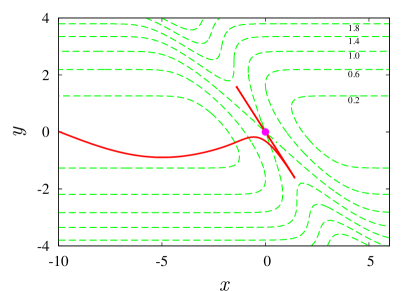
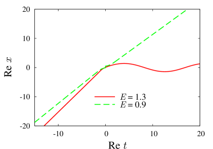
(a)                                                                     (b)

Figure 1: (a) The contour plot of the potential (dashed lines) and the real part of the tunneling trajectory at $E=1.3$, $E_{y}=0.05$ (solid line). The saddle point is marked by the thick dot. (b) Time evolution of $\mathrm{Re}\,x$ for two complex trajectories with $E_{y}=0.05$ and different values of total energy, $E=0.9$ and $1.3$. Note that $E_{c}(E_{y}=0.05)\approx 1.1$.

We are interested in tunneling transitions of quantum particle between the asymptotic regions $x\to-\infty$ and $x\to+\infty$ of the potential (in- and out- regions respectively). In the in-region the particle evolves with constant momentum in the $x$ direction oscillating along the $y$ axis. The corresponding in-state is fixed by the total energy $E$ and the energy of $y$ oscillations $E_{y}$. Similarly, the out-state can be fully characterized by $E$ and $E_{y}^{f}$, where $E_{y}^{f}$ is the final oscillator energy. In what follows we will often omit the specification of the out-state and consider the total (inclusive) probability of tunneling into the region $x\to+\infty$.

The height of the potential barrier separating the in- and out- regions is $V_{0}=1$. It is given by the value of the potential at the saddle point $(x,y)=(0,0)$. At $E<V_{0}$ the classical transitions between the regions are forbidden energetically, and their underlying mechanism is potential tunneling. On the other hand, it is shown in Ref. [38] that classical over–barrier transitions between the asymptotic regions take place at $E>E_{b}(E_{y})$, where $E_{b}(E_{y})$ is larger than $V_{0}$. Hence, at intermediate energies $V_{0}<E<E_{b}(E_{y})$ the transitions are in the regime of dynamical tunneling, which we are interested in.

As we have already discussed in the Introduction, the multidimensional processes of dynamical tunneling, such as ours, generically proceed via sphaleron–driven mechanism at sufficiently high energies. Let us illustrate the new mechanism in the model (2) comparing the behavior of semiclassical solutions at low and high energies [26]. Consider the inclusive tunneling transition from the state $|E,E_{y}\rangle$ into the out-region $x\to+\infty$. We postpone the consistent formulation of the semiclassical method till Sec. 4. The only fact we need here is that any tunneling process is specified by a certain complex trajectory — solution to the (complexified) classical equations of motion. The latter should interpolate between the in- and out- regions of the process.

Fig. 1b shows the complex trajectories describing tunneling transitions at $E_{y}=0.05$ and two values of total energy, $E=0.9$ and $1.3$. [The real part of the trajectory with $E=1.3$ is also depicted in Fig. 1a.] The behavior of the two trajectories is drastically different. While the low–energy trajectory interpolates between the asymptotic regions $x\to\pm\infty$, the solution with $E=1.3$ gets stuck at finite $x$ approaching the unstable periodic orbit as $t\to+\infty$. The latter orbit is precisely the sphaleron discussed in the Introduction; it describes oscillations around the saddle point of the potential, see Fig. 1a. Clearly, the high–energy trajectory of Fig. 1 describes only half of the transition process, since it does not arrive into the out-region. Trajectory corresponding to the other half can be obtained by adding to the unstable periodic orbit infinitesimally small momentum in the direction of the out-region and evolving the system classically. Thus constructed, the overall semiclassical evolution involves two trajectories which describe creation and subsequent decay of the sphaleron. This evolution corresponds to the mechanism of sphaleron–driven tunneling.

One finds [26] that there exists the critical value $E=E_{c}(E_{y})$ of total energy which separates the regions of qualitatively different behavior of tunneling trajectories. Namely, the trajectories interpolate between the in- and out- regions at $E<E_{c}(E_{y})$ and approach the sphaleron orbit at $E_{c}(E_{y})<E<E_{b}(E_{y})$. This means that the mechanism of transition changes from potential to sphaleron–driven tunneling as the energy crosses the critical value. From the physical viewpoint $E_{c}(E_{y})$ can be understood as the energy of “phase transition” between the two regimes of tunneling. We remark that the energies of sphaleron orbits and thus the critical energy for the sphaleron–driven tunneling exceed the height of the potential barrier. Therefore, the new mechanism is relevant only in the case of dynamical tunneling.

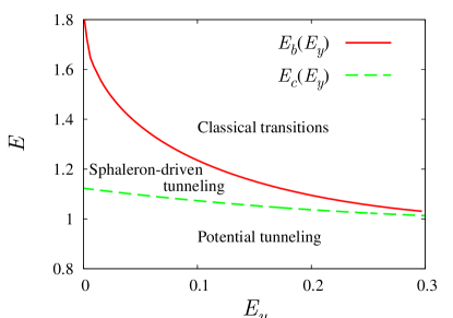
Figure 2: Regions in the plane of in–state quantum numbers corresponding to the potential and sphaleron–driven tunneling mechanisms.

The region $E_{c}(E_{y})<E<E_{b}(E_{y})$ corresponding to the sphaleron–driven tunneling in the model (2) is shown in Fig. 2. The value of $E_{c}(E_{y})$ is found numerically by computing the complex trajectories at different energies and investigating their stability.

3 Experimental signatures

In this Section we show that the mechanism of sphaleron–driven tunneling leads to two observable effects which in principle can be used for identification of the new mechanism in future experiments. Both effects are related to the fact that the relevant semiclassical solutions are unstable. We illustrate our findings in the model (2) using the exact quantum mechanical results. The exact calculations of this and the subsequent sections are based on the numerical solution of time–independent Schrödinger equation, see Refs. [38, 16, 39] for the numerical method and Fortran 90 code.

The first signature of sphaleron–driven tunneling is the direct consequence of the semiclassical analysis which will be presented in Sec. 4. We find that the sphaleron–driven mechanism changes the power–law dependence of the transmission probability on $\hbar$ compared to the case of potential tunneling. To be concrete, let us discuss inclusive tunneling transitions in the model (2). Then, the prefactor $A$ of the probability is proportional to $\hbar^{1/2}$ and $\hbar$ in the cases of potential and sphaleron–driven tunneling respectively.

The physics behind the additional power–law suppression becomes clear if one uses the qualitative analogy with the classically allowed creation of unstable state. The latter process considered at the classical level requires fine tuning of the Cauchy data. As a consequence, only a small part of the in-state wave function contributes into the amplitude of the process. This results in the additional suppression of the probability. On general grounds one expects similar formal suppression in the case of sphaleron–driven tunneling.

Experimentally, one can try to observe the unusual power–law dependence on $\hbar$ by analyzing the probability graph ${\cal P}(\hbar)$. Note that the value of the semiclassical parameter which we denote by $\hbar$ is, in principle, adjustable in experiments. Indeed, the magnitude of quantum fluctuations is measured by the dimensionless ratio of the Planck constant to a certain combination of parameters characterizing the system. Changing the latter parameters in an appropriate way, one alters the value of the semiclassical parameter $\hbar$ without affecting the classical dynamics of the system.

To illustrate this point consider the system (2). The key quantity which enters into the semiclassical expansion is the ratio of the action of the system to the Planck constant. Restoring the dimensionful units we obtain

$$\frac{S}{\hbar_{0}}=\frac{1}{\hbar_{0}}\int dt\left(\frac{M{\dot{\boldsymbol{x}}}^{2}}{2}-\frac{M\omega_{0}^{2}y^{2}}{2}-V_{0}{\rm e}^{-(x+y)^{2}/2L^{2}}\right)\;,$$

where $\hbar_{0}$ stands for the physical Planck constant. In terms of dimensionless variables this expression reads

$$\frac{S}{\hbar_{0}}=\frac{1}{\hbar}\int d\tilde{t}\left(\frac{{\dot{\tilde{\boldsymbol{x}}}}^{2}}{2}-\frac{\omega^{2}\tilde{y}^{2}}{2}-{\rm e}^{-(\tilde{x}+\tilde{y})^{2}/2}\right)\;,$$

where $\hbar=\hbar_{0}/\sqrt{MV_{0}L^{2}}$, $\omega^{2}=ML^{2}\omega_{0}^{2}/V_{0}$. The effective frequency $\omega$ completely determines the classical dynamics. On the other hand, the effective Planck constant $\hbar$ is given by an independent combination of parameters.

One can hardly hope to extract directly the additional factor $\hbar^{1/2}$ from the experimental data on transmission probability: it is almost impossible to identify the weak power–law dependence on top of the leading semiclassical exponent. We suggest an indirect method. Namely, consider the quantity

$$F_{QM}=-\hbar\log({\cal P}/\hbar^{1/2}).$$

In the regime of potential tunneling ($A\propto\hbar^{1/2}$) $F_{QM}$ is almost independent of $\hbar$ at small values of the latter. On the other hand, $F_{QM}\simeq-\frac{1}{2}\hbar\log\hbar+\mbox{const}$ whenever the new tunneling mechanism is involved. The difference between the two cases is seen in Fig. 3, where the dependences of $F_{QM}$ on the total energy $E$ are shown for several values of $\hbar$. The graphs in Fig. 3 coincide at energies somewhat smaller than $E_{c}$ (say, at $E\lesssim 1$), while at $E>E_{c}$ a clear difference between the graphs appears. We remark that the change in the behavior of the exact tunneling probability is gradual, in spite of the fact that the complex trajectories have distinct structure at $E<E_{c}$ and $E>E_{c}$. We discuss this point and derive the appropriate uniform formula in Sec. 4.3.

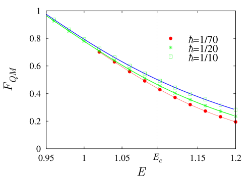
Figure 3: The probability logarithm $F_{QM}=-\hbar\log({\cal P}/\hbar^{1/2})$ plotted as a function of total energy for several values of $\hbar$ and $E_{y}=0.05$. Points represent the exact quantum mechanical results; the interpolating lines are drawn for convenience. The critical energy is shown by dashed vertical line.

Another signature of the sphaleron–driven mechanism was first pointed out in Refs. [25, 30]. One notes that the second stage of sphaleron–driven transition, the decay of the sphaleron orbit, proceeds classically and does not affect the leading suppression exponent $F$ of the probability. In addition, the sphaleron, being unstable, can evolve at the classical level into the out-states with different values of oscillator energy $E_{y}^{f}$. Classical trajectories corresponding to these evolutions are obtained by adding small momentum in the direction of the out-region at different points of the sphaleron orbit. One concludes that in the case of sphaleron–driven tunneling the distribution over final oscillator energies is almost constant in some region $E_{y,1}^{f}<E_{y}^{f}<E_{y,2}^{f}$. The latter region corresponds to the decays of the sphaleron along different classical trajectories.

Note that the above feature is in sharp contrast with the properties of final states in the standard case of potential tunneling. Namely, in a typical situation the complex trajectory describing transmission through the barrier is unique, and the corresponding out-state wave function forms sharply peaked Gaussian distribution around some optimal value $E_{y}^{f}=\langle E_{y}^{f}\rangle$.

To illustrate explicitly the effect of anomalously wide final states in the case of sphaleron–driven tunneling, we consider transitions between the exclusive in- and out- states which have definite energies of $y$ oscillator, $E_{y}$ and $E_{y}^{f}$ respectively, and the same total energy $E$. Then, we fix the initial state ($E$ and $E_{y}$) and analyze the dependence of the exact exclusive probability ${\cal P}_{e}$ on $E_{y}^{f}$. This dependence is shown in Fig. 4 in logarithmic scale for several values of $E$. One immediately sees in Fig. 4a that the width of the out-state distribution grows as the value of total energy approaches $E_{c}(E_{y})$ from below. In particular, a flat plateau gradually develops in the right side of the distribution. At energies higher than critical the plateau is wide and corresponds to the maximum probability of tunneling. Moreover, the graphs become flatter as the value of $\hbar$ decreases, see Fig. 4b.

One sees another feature of the new tunneling mechanism: the short–scale fluctuations in the right and left parts of the plateaux in Fig. 4b. This is the hallmark of quantum interference phenomena, which seem to be important for complete understanding of exclusive processes at $E>E_{c}(E_{y})$. We discuss this point in Sec. 5.

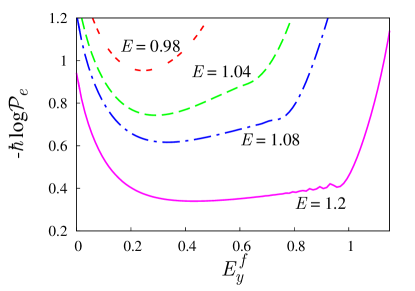
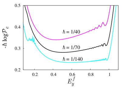
(a)                                                                     (b)

Figure 4: Distributions of the logarithm of exclusive tunneling probability over the out-state quantum number $E_{y}^{f}$. The graphs are plotted at $E_{y}=0.05$ and: (a) $\hbar=1/40$ and four values of total energy; (b) $E=1.2$ and different values of $\hbar$. Note that $E_{c}(E_{y}=0.05)\approx 1.1$.

4 Modified semiclassical technique

In this section we describe the semiclassical technique adapted to the analysis of sphaleron–driven tunneling. We start by reviewing the path integral derivation of the standard method of complex trajectories [22]. Then, we manipulate with the path integral and obtain the modified semiclassical expressions in the case of sphaleron–driven tunneling.

For simplicity we assume that the system undergoing tunneling transition is similar to the model of Sec. 2. Throughout this section we consider tunneling between the asymptotic in- and out- regions of two–dimensional waveguide potential, where the in-state of the process $|E,\,E_{y}\rangle$ is fixed and the final state is inclusive. It is worth noting that both the standard and modified semiclassical methods are completely general and the semiclassical formulas of this section can be generalized to other systems. In particular, the modified method was applied to the case of chaotic tunneling in Ref. [16] and to field theory in Ref. [32].

4.1 The standard method

Semiclassical calculations within the method of complex trajectories proceed as follows. One reduces the problem of computing the tunneling probability to a problem of finding the complex trajectory $\boldsymbol{x}^{(s)}(t)$ — complex solution to the classical equations of motion with certain boundary conditions. In practice this solution is obtained numerically. Then, tunneling probability is given by Eq. (1) where $F$ and $A$ are certain functionals of $\boldsymbol{x}^{(s)}(t)$. In this section we derive the boundary conditions for $\boldsymbol{x}^{(s)}(t)$ and expressions for the functionals $F$, $A$ in the standard case of potential tunneling.

In order to compute the inclusive tunneling probability we first obtain the semiclassical expression for the final state of the tunneling process. The wave function $\Psi_{f}$ of the final state has the form,

$$\Psi_{f}(\boldsymbol{x}_{f})=\langle\boldsymbol{x}_{f}|\,\mathrm{e}^{-iH(t_{f}-t_{i})/\hbar}\,|E,\,E_{y}\rangle=\int d\boldsymbol{x}_{i}\,\langle\boldsymbol{x}_{f}|\,\mathrm{e}^{-iH(t_{f}-t_{i})/\hbar}\,|\boldsymbol{x}_{i}\rangle\,\Psi_{i}(\boldsymbol{x}_{i})\;,$$ (3)

where $\boldsymbol{x}=(x,\,y)$, while $\Psi_{i}(\boldsymbol{x}_{i})=\langle\boldsymbol{x}_{i}|E,\,E_{y}\rangle$ is the in-state wave function. Below we assume implicitly that $\Psi_{i}$ and $\Psi_{f}$ have support in the in- and out- asymptotic regions respectively. One uses the path integral representation for the quantum propagator in Eq. (3) and writes,

$$\Psi_{f}(\boldsymbol{x}_{f})=\left.\int d\boldsymbol{x}_{i}\,\Psi_{i}(\boldsymbol{x}_{i})\,\int[d\boldsymbol{x}]\right|_{\boldsymbol{x}_{i}}^{\boldsymbol{x}_{f}}\,\mathrm{e}^{iS[\boldsymbol{x}]/\hbar}\;,$$ (4)

where $S$ stands for the classical action of the system. One observes that at small $\hbar$ the integrand in Eq. (4) contains fast–oscillating exponent; thus, the respective integral can be evaluated by the saddle–point method. To keep the discussion short, we defer the details of the saddle–point integration to appendix A; here we quote the result. One finds the extremum of the leading exponent in Eq. (4), which is represented by the trajectory $\boldsymbol{x}^{(s)}(t)$ going between the in- and out- regions. This trajectory is generically complex. It satisfies the classical equations of motion $\delta S/\delta\boldsymbol{x}(t)=0$ and arrives at a given point $\boldsymbol{x}=\boldsymbol{x}_{f}$ at $t=t_{f}$. The boundary conditions at $t=t_{i}$ for $\boldsymbol{x}^{(s)}(t)$ are obtained from the saddle–point integration over $\boldsymbol{x}_{i}$; they fix the values of in-state quantum numbers,

$$E_{y}=(\dot{y}_{i}^{2}+\omega^{2}y_{i}^{2})/2\;,\qquad\qquad E=\dot{x}_{i}^{2}/2+E_{y}\;,$$ (5)

where the subscript $i$ marks the quantities evaluated at $t=t_{i}$. For brevity we omit the superscript $(s)$ of the semiclassical trajectory in Eq. (5) and in what follows.

As the result of integration in Eq. (4), one finds the semiclassical wave function of the final state,

$$\Psi_{f}(\boldsymbol{x}_{f})=D^{-1/2}\cdot\exp\left\{{\frac{i}{\hbar}(S[\boldsymbol{x}]+B_{i}[\boldsymbol{x}])+\frac{i\pi}{4}}\right\}\;,$$ (6)

where $B_{i}$ is the in-state contribution to the exponent and $D$ represents the prefactor determinant, see Eqs. (50), (63) in appendix A for explicit expressions. Note that the leading exponent $S+B_{i}$ in Eq. (6) is evaluated on the saddle–point trajectory $\boldsymbol{x}(t)$.

The inclusive probability ${\cal P}$ of transmission is equal to the total flux of the out-wave (6) through the distant line $x_{f}=x_{f}^{(0)}$, where $x_{f}^{(0)}$ is large and positive. Semiclassically, one writes,

$${\cal P}=\int dy_{f}\,|\Psi_{f}(\boldsymbol{x}_{f})|^{2}\,\mathrm{Re}\,\dot{x}_{f}\;,$$ (7)

where we used the fact that $\partial S/\partial x_{f}=\dot{x}_{f}$. The integral in the above expression is again computed by the saddle–point technique. In appendix A we show that the extremum of the leading exponent in Eq. (7) is achieved when

$$x_{f}=x_{f}^{(0)}\;,\qquad\qquad\mathrm{Im}\,\dot{y}_{f}=\mathrm{Im}\,y_{f}=0\;.$$ (8)

Equations (8) fix the boundary conditions at $t=t_{f}$ for the semiclassical trajectory.

After the saddle–point integration in Eq. (7) one finally arrives at the familiar semiclassical expression (1) for the tunneling probability, where the leading exponent is

$$F_{pot}=2\,\mathrm{Im}(S+B_{i})\;.$$ (9)

Note that we mark all the standard semiclassical expressions with the subscript $pot$ which stands for “potential tunneling”.

The prefactor $A_{pot}$ is computed as follows (see appendix A for the derivation). One finds two independent perturbations $\delta\boldsymbol{x}^{(1)}(t)$ and $\delta\boldsymbol{x}^{(2)}(t)$ in the background of the complex trajectory $\boldsymbol{x}(t)$. These perturbations satisfy the linearized classical equations of motion,

$$\delta\ddot{\boldsymbol{x}}^{(n)}+\hat{V}^{\prime\prime}(\boldsymbol{x}(t))\delta\boldsymbol{x}^{(n)}=0\;,\qquad\qquad n=1,2$$ (10)

with certain Cauchy data at $t=t_{f}$. After evolving $\delta\boldsymbol{x}^{(n)}(t)$ back in time from $t=t_{f}$ to $t=t_{i}$, one computes the prefactor by the formula

$$A_{pot}=\frac{\hbar^{1/2}\omega}{\sqrt{4\pi\,\mathrm{Im}(\delta E_{y}[\delta\boldsymbol{x}^{(1)}]\cdot\delta E_{y}^{*}[\delta\boldsymbol{x}^{(2)}])}}\;,$$ (11)

where the linear functional

$$\delta E_{y}[\delta\boldsymbol{x}]=\dot{y}_{i}\delta\dot{y}_{i}+\omega^{2}y_{i}\delta y_{i}$$ (12)

measures the change in the initial oscillator energy $E_{y}$ due to the perturbation $\delta\boldsymbol{x}(t)$. We stress that $\delta E_{y}[\delta\boldsymbol{x}^{(n)}]$ involves perturbations in the in-region, while the Cauchy data for $\delta\boldsymbol{x}^{(n)}(t)$ are set at $t=t_{f}$. We also note that the prefactor (11) is explicitly proportional to $\hbar^{1/2}$; this fact was used in the previous section.

The standard semiclassical calculation is summarized as follows. One finds the complex trajectory $\boldsymbol{x}(t)$ satisfying the classical equations of motion with the boundary conditions (5), (8). Our numerical method for finding the trajectory is presented in appendix B. The suppression exponent $F_{pot}$ of the probability is given by the value of the functional (9) on the trajectory $\boldsymbol{x}(t)$. Then, one considers the linear perturbations around the semiclassical trajectory and finds the prefactor $A_{pot}$ using the expression (11).

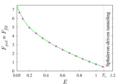
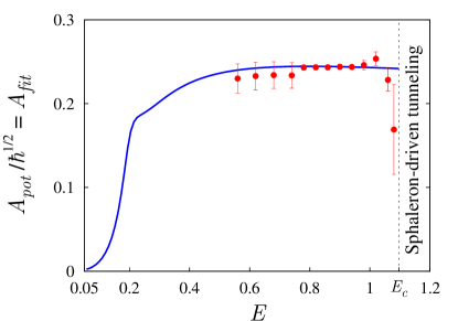
(a)                                                                     (b)

Figure 5: The semiclassical (lines) and exact quantum mechanical (points) results for (a) leading suppression exponent and (b) prefactor; $E_{y}=0.05$. Errorbars represent uncertainty of the fit (13).

Before proceeding to the case of sphaleron–driven tunneling, we demonstrate explicitly that the semiclassical expressions (9), (11) produce correct values of suppression exponent and prefactor. To this end, we calculate the exact probability of transition by solving numerically the stationary Schrödinger equation (see Refs. [38, 16] for the numerical method). The exact values of $\cal P$ are computed at several $\hbar$. Then, the dependence ${\cal P}(\hbar)$ is fitted with the formula

$$-\hbar\log({\cal P}/\hbar^{\gamma})=F_{fit}-\hbar\log A_{fit}+\hbar^{2}C_{fit}\;,$$ (13)

where $\gamma=1/2$ and the last term accounts for the higher-order semiclassical corrections. The fit produces the “exact” values $F_{fit}$, $A_{fit}$ of the suppression exponent and prefactor; they should coincide with the corresponding semiclassical quantities. In Fig. 5 we compare the semiclassical results computed by Eqs. (9), (11) with those extracted from the fit (13). One observes remarkable agreement. It is worth noting that the fit (13) is extremely sensitive to the assumed $\hbar$-dependence of the prefactor. In particular, if one erroneously uses $\gamma=0$ or $\gamma=1$ in Eq. (13), the value of prefactor extracted from the fit becomes close to zero or extremely large. Hence, the graph in Fig. 5b confirms, in particular, the qualitative formula $A_{pot}\propto\hbar^{1/2}$.

4.2 Modification

At high energies tunneling proceeds by the new mechanism based on qualitatively new properties of semiclassical trajectories. Namely, at $E>E_{c}(E_{y})$ the trajectories get attracted to the unstable sphaleron orbit and thus become unstable themselves.

The instability of complex trajectories sets obstacles for the semiclassical description. The most important difficulty is related to the calculation of the prefactor $A_{pot}$. Equation (11) implies that $A_{pot}$ is inversely proportional to the values of linear perturbations $\delta\boldsymbol{x}^{(n)}$ at $t=t_{i}$, while the Cauchy data for $\delta\boldsymbol{x}^{(n)}$ are set at $t=t_{f}$. On the other hand, linear perturbations in the background of unstable trajectory contain exponentially growing part. Thus, at $E>E_{c}(E_{y})$ when the complex trajectory spends infinite time interval in the vicinity of the sphaleron, the formula (11) gives $A_{pot}=0$. This means that Eq. (11) is incorrect in the case of sphaleron–driven tunneling and suggests that the prefactor is suppressed by an additional power of $\hbar$.

The main idea of the modified semiclassical method was proposed in Ref. [28]; it is close in spirit to the constrained instanton technique of Ref. [40]. Namely, we evaluate the path integral (4) for the tunneling amplitude in two steps. First, we integrate over paths spending a given time $\tau$ in the vicinity of the sphaleron. Second, we integrate over $\tau$.

The above manipulations with the path integral lead to the following method. At the first step we obtain certain modified boundary value problem for a family of complex trajectories labeled by the parameter $\tau$. These trajectories are stable and interpolate between the asymptotic regions $x\to\pm\infty$. The second step produces expressions for the suppression exponent $F_{sph}$ and prefactor $A_{sph}$ in the sphaleron–driven case. These expressions relate the values of $F_{sph}$ and $A_{sph}$ to limits $\tau\to+\infty$ of certain functionals evaluated on the modified trajectories.

One introduces the functional $\tau=T_{int}[\boldsymbol{x}]$ which, roughly speaking, measures the time spent by the path $\boldsymbol{x}(t)$ in the region of non–trivial dynamics. We call $T_{int}$ interaction time. It has the following properties. First, $T_{int}$ is positive–definite for real paths. Second, it is finite for any real path satisfying $x\to\pm\infty$ as $t\to\pm\infty$ and infinite otherwise. The simplest choice is

$$T_{\mathrm{int}}[\boldsymbol{x}]=\int dt\,f(\boldsymbol{x}(t))\;,$$ (14)

where the function $f(\boldsymbol{x})>0$ vanishes at $x\to\pm\infty$. We use

$$f(\boldsymbol{x})=\mathrm{exp}\,\left\{-(x+y)^{2}/2\right\}$$

in the model (2).

Consider the path integral (4) for the final state. One inserts into the integrand of Eq. (4) the unity factor

$$1=\int_{0}^{+\infty}d\tau\,\delta(T_{\mathrm{int}}[\boldsymbol{x}]-\tau)=\int_{0}^{+\infty}d\tau\int_{i\infty}^{-i\infty}\frac{id\epsilon}{2\pi\hbar}\,\mathrm{e}^{-\epsilon T_{\mathrm{int}}[\boldsymbol{x}]/\hbar+\epsilon\tau/\hbar}\;,$$ (15)

where the Fourier representation of the $\delta$–function was used in the second equality. Expression (4) takes the form,

$$\Psi_{f}(\boldsymbol{x}_{f})=\int_{0}^{+\infty}d\tau\int_{i\infty}^{-i\infty}\frac{id\epsilon}{2\pi\hbar}\,\mathrm{e}^{\epsilon\tau/\hbar}\left\{\left.\int d\boldsymbol{x}_{i}\,\Psi_{i}(\boldsymbol{x}_{i})\int[d\boldsymbol{x}]\right|_{\boldsymbol{x}_{i}}^{\boldsymbol{x}_{f}}\mathrm{e}^{i(S[\boldsymbol{x}]+i\epsilon T_{int}[\boldsymbol{x}])/\hbar}\right\}\;,$$ (16)

where we changed the order of integrations. One notes that the integral in brackets is exactly the same as in Eq. (4) up to the substitution

$$S[\boldsymbol{x}]\to S_{\epsilon}[\boldsymbol{x}]\equiv S[\boldsymbol{x}]+i\epsilon T_{\mathrm{int}}[\boldsymbol{x}]\;.$$ (17)

This integral is evaluated by the saddle–point method in the same way as the integral in Eq. (4). Namely, one finds the regularized trajectory $\boldsymbol{x}_{\epsilon}(t)$ which extremizes the modified action $S_{\epsilon}$ and arrives at the point $\boldsymbol{x}_{f}$ at $t=t_{f}$. The initial conditions for the trajectory are still given by Eqs. (5), since the evolution in the in-region is not affected by the functional $T_{int}$. The result of integration in Eq. (16) is

$$\Psi_{f}(\boldsymbol{x}_{f})=\int_{0}^{+\infty}d\tau\int_{i\infty}^{-i\infty}\frac{id\epsilon}{2\pi\hbar}\,\mathrm{e}^{\epsilon\tau/\hbar}\cdot D_{\epsilon}^{-1/2}\cdot\exp\left\{{\frac{i}{\hbar}(S_{\epsilon}[\boldsymbol{x}_{\epsilon}]+B_{i}[\boldsymbol{x}_{\epsilon}])+\frac{i\pi}{4}}\right\}\;,$$ (18)

cf. Eq. (6). The prefactor $D_{\epsilon}$ in this equation is given by the same determinant formula as $D$, but with the substitution $S\to S_{\epsilon}$, $\boldsymbol{x}(t)\to\boldsymbol{x}_{\epsilon}(t)$.

Let us remark on the representation (18). One keeps in mind that the integrand in Eq. (18) accounts for the contribution of paths which spend a given time $\tau$ in the region of finite $x$ (interaction region). In particular, this is true for the saddle–point trajectory $\boldsymbol{x}_{\epsilon}(t)$. The latter interpolates directly between the in- and out- regions $x\to\pm\infty$ and thus is stable. Note that the stabilization of complex trajectory is achieved by the modification of the classical equations of motion. Namely, the substitution (17) modifies the potential of the system

$$V(\boldsymbol{x})\to V(\boldsymbol{x})-i\epsilon f(\boldsymbol{x})\;.$$

We will see below that the relevant values of $\epsilon$ are real; thus, $\boldsymbol{x}_{\epsilon}(t)$ describes evolution in complex potential.

The rest of the calculation proceeds as follows. One evaluates the saddle–point integral with respect to $\epsilon$. The integral over interaction time is kept in front of the formula. This ensures stability of complex trajectories. The resulting expression for $\Psi_{f}$ is substituted into the tunneling probability (7). A subtle point is that, since ${\cal P}$ involves the square of the out-state, one obtains at this stage two integrals over interaction times $\tau$, $\tau^{\prime}$, where the latter comes from $\Psi_{f}^{*}$. One of these integrals can be computed by the saddle–point technique. Indeed, returning to the original expression for the tunneling probability in terms of the integral over real paths, one sees that fixing the sum $\tau_{+}=(\tau+\tau^{\prime})/2$ is sufficient to make both interaction times $\tau$ and $\tau^{\prime}$ finite. Thus, we change the integration variables to $\tau_{+}$ and $\tau_{-}=\tau-\tau^{\prime}$ and evaluate the saddle–point integrals over $\tau_{-}$ and over the final state. In this way we are left with the single integral over $\tau_{+}$.

We leave the details of the above computation to appendix C and discuss the result. First, one arrives at the saddle–point conditions

$$\mathrm{Re}\,T_{int}[\boldsymbol{x}_{\epsilon}]=\tau_{+}\;,\qquad\epsilon=\epsilon^{*}\;,$$ (19)

which come from the integrals over $\epsilon$ and $\tau_{-}$ respectively. The integral over out-states produces, as before, the boundary conditions (8) at $t=t_{f}$ for $\boldsymbol{x}_{\epsilon}(t)$. Note that the first of Eqs. (19) implies, in particular, that $\boldsymbol{x}_{\epsilon}(t)$ is stable. The result for the probability is

$${\cal P}=\int_{0}^{+\infty}\frac{d\tau_{+}}{\sqrt{\pi\hbar}}\left[-\frac{d\epsilon}{d\tau_{+}}\right]^{1/2}\cdot A_{pot,\,\epsilon}\;\mathrm{e}^{-(F_{pot,\epsilon}-2\epsilon\tau_{+})/\hbar}\;,$$ (20)

where the suppression exponent $F_{pot,\epsilon}$ and prefactor $A_{pot,\epsilon}$ are computed by the same formulas (9) and (11) as before, but with the substitution $S\to S_{\epsilon}$. Note that the latter substitution implies that both the classical equations of motion and linearized equations (10) are modified.

We now proceed to the second step of the calculation and consider the integral over the interaction time $\tau_{+}$. One makes an important observation: the values of $\tau_{+}$ and $\epsilon(\tau_{+})$ are related by the Legendre transformation. Indeed, by construction the configuration $\{\boldsymbol{x}_{\epsilon}(t),\;\epsilon(\tau_{+})\}$ corresponds to the extremum of the leading exponent $F_{\epsilon}=F_{pot,\epsilon}-2\epsilon\tau_{+}$ in Eq. (20), and the respective derivatives of $F_{\epsilon}$ are equal to zero. Thus,

$$\frac{dF_{\epsilon}}{d\tau_{+}}=\frac{\partial}{\partial\tau_{+}}(F_{pot,\,\epsilon}-2\epsilon\tau_{+})=-2\epsilon\;,$$ (21)

where only the explicit dependence of $F_{\epsilon}$ on $\tau_{+}$ was taken into account in the last equality. Due to the property (21), the integral in Eq. (20) is saturated at $\epsilon=0$. This point corresponds to the original semiclassical equations: recall that the modification term in the classical action, Eq. (17), is proportional to $\epsilon$. One concludes that the integral for the tunneling probability is saturated in the vicinity of the original complex trajectory at $\epsilon=0$.

So far in our calculation we did not make any reference to the particular tunneling mechanism. Thus, Eq. (20) can be used in cases of both potential and sphaleron–driven tunneling. The difference between the two mechanisms becomes crucial in the evaluation of the integral over $\tau_{+}$. In the standard case of potential tunneling the trajectory at $\epsilon=0$ is stable and corresponds to the finite value of interaction time $\tau_{+}$; one takes the integral in Eq. (20) by the saddle–point method and arrives at the expressions (9), (11) from the previous subsection. The case of sphaleron–driven tunneling is considerably different, because the time interval spent by the trajectory in the vicinity of the sphaleron tends to infinity as $\epsilon\to+0$. Thus, the integral in Eq. (20) is saturated by the end–point of the integration interval $\tau_{+}\to+\infty$. Using the appropriate asymptotic expression for the integral, one obtains Eq. (1) with

$$F_{sph}=\lim_{\epsilon\to+0}F_{\epsilon}\;,$$ (22a)

$$A_{sph}=\hbar^{1/2}\lim_{\epsilon\to+0}\frac{A_{pot,\,\epsilon}}{\epsilon\sqrt{-4\pi\frac{d\mathrm{Re}\,T_{int}[\boldsymbol{x}_{\epsilon}]}{d\epsilon}}}\;,$$ (22b)

where we mark the quantities corresponding to the new mechanism with the subscript $sph$. Note that the prefactor $A_{pot,\,\epsilon}$ is computed by the formula (11) with modification (17), while the exponent

$$F_{\epsilon}=F_{pot,\,\epsilon}-2\epsilon\tau_{+}=2\mathrm{Im}(S[\boldsymbol{x}_{\epsilon}]+B_{i}[\boldsymbol{x}_{\epsilon}])$$

is given by the value of the original action on the modified trajectory. Let us remark that the limit $\epsilon\to+0$ in Eqs. (22) does actually exist; this is shown analytically in appendix D. One observes that the expression (22b) for the prefactor is very different from that in the case of potential tunneling. In particular, $A_{sph}\propto\hbar^{1/2}A_{pot}$.

To summarize, we derived the following method of calculating the probability of sphaleron–driven tunneling. One modifies the classical action of the system by adding purely imaginary term proportional to the small regularization parameter $\epsilon>0$, see Eq. (17). Then one solves the modified equations of motion with the original boundary conditions (5), (8) and finds the modified complex trajectory $\boldsymbol{x}_{\epsilon}(t)$. This trajectory interpolates between the asymptotic regions $x\to\pm\infty$ and is stable. The modified values of the suppression exponent $F_{pot,\,\epsilon}$ and prefactor $A_{pot,\,\epsilon}$ are computed by the same formulas as before, Eqs. (9) and (11), but with the substitution $S\to S_{\epsilon}$. The final result for the tunneling probability is obtained in the limit $\epsilon\to+0$, see Eqs. (22). We call the above modified semiclassical method by $\epsilon$–regularization technique [26].

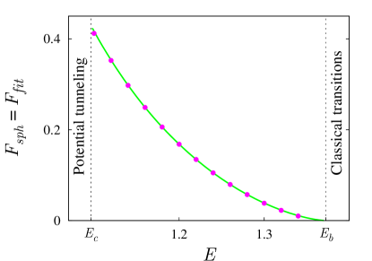
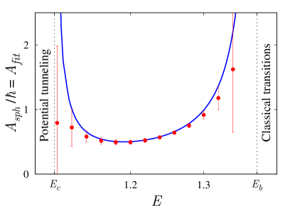
(a)                                                                     (b)

Figure 6: (a) Suppression exponent and (b) prefactor in the case of sphaleron–driven tunneling, $E>E_{c}(E_{y})$; $E_{y}=0.05$. The points are extracted from the fit (13), while the lines stand for the semiclassical results, Eqs. (22). The vertical dotted lines bound the range of energies for sphaleron–driven tunneling.

We perform straightforward check of the modified semiclassical method by comparing the semiclassical predictions (22) with the results of the exact quantum mechanical computations. The latter are used to extract the values of the suppression exponent and prefactor by the fitting procedure described in the previous subsection, where $\gamma=1$ in Eq. (13). The comparison is shown in Fig. 6. The observed agreement between the semiclassical and quantum mechanical results supports the modified semiclassical technique. In particular, we checked that the fit (13) produces unacceptably large values of the prefactor if one erroneously assumes the same $\hbar$–dependence $\gamma=1/2$ as in the case of potential tunneling. Thus, the scaling $A_{sph}\propto\hbar$ is confirmed.

4.3 Uniform approximation

Our expressions for $A_{pot}$ and $A_{sph}$ imply apparent discontinuity of the semiclassical probability across the critical energy; on the other hand, the exact quantum probability is a smooth function of energy. As a consequence, the $\hbar$–dependences $A_{pot}\propto\hbar^{1/2}$ and $A_{sph}\propto\hbar$ fail to describe the quantum mechanical data in the immediate vicinity of $E_{c}(E_{y})$. [This is seen in Figs. 5b, 6b, where the quality of the fit (13) becomes worse as $E\to E_{c}(E_{y})$.] One observes that both the standard and modified formulas are invalid at $E\approx E_{c}(E_{y})$.

In this section we derive the uniform asymptotic formula for the tunneling probability which is applicable in the vicinity of $E_{c}(E_{y})$. Our formula has the form (cf. Ref. [9]),

$${\cal P}_{uni}=\left\{\begin{array}[]{ll}{\cal M}_{pot}\cdot{\cal P}_{pot}&\;\;\mbox{at}\;\;E<E_{c}(E_{y})\;,\\ {\cal M}_{sph}\cdot{\cal P}_{sph}&\;\;\mbox{at}\;\;E>E_{c}(E_{y})\;,\end{array}\right.$$ (23)

where ${\cal M}_{pot}$ and ${\cal M}_{sph}$ are the correction factors in the cases of potential and sphaleron–driven tunneling respectively. We will find that ${\cal M}_{pot,\,sph}\approx 1$ at $|E-E_{c}|\gg\hbar^{1/2}$; thus, the formula (23) is relevant in the small region of width $\Delta E\sim\hbar^{1/2}$ around the critical point. We stress that the uniform probability ${\cal P}_{uni}$ is continuous at $E=E_{c}(E_{y})$.

We obtain the desired approximation by examining the integral over $\tau_{+}$ for the tunneling probability, Eq. (20). Recall that Eq. (20) is applicable in both cases of potential and sphaleron–driven tunneling. To make the discussion transparent, we change the integration variable to

$$w(\tau_{+})=\frac{1}{\sqrt{\pi\hbar}}\int_{\tau_{+}}^{+\infty}d\tau_{+}^{\prime}\,\sqrt{-d\epsilon^{\prime}/d{\tau^{\prime}_{+}}}\cdot A_{pot,\,\epsilon^{\prime}}\;.$$ (24)

Note that the limiting values $\tau_{+}=0$ and $\tau_{+}\to+\infty$ correspond respectively to $w=w_{0}>0$ and $w\to+0$. In new terms the integral (20) takes a particularly simple form,

$${\cal P}=\int_{0}^{w_{0}}dw\,\mathrm{e}^{-F_{\epsilon}(w)/\hbar}\;,$$ (25)

where the leading semiclassical exponent is now considered as function of $w$.

The difference between the two mechanisms of tunneling is now understood as follows. At small energies the integral (25) is saturated by the saddle point $w=w_{s}>0$. The value of $w_{s}$ decreases with energy, so that at $E=E_{c}(E_{y})$ the saddle point crosses the boundary $w=0$ and leaves the integration interval. At $E>E_{c}(E_{y})$ the saddle point $w_{s}$ is situated outside the region of integration.

Consider the Taylor series expansions of the semiclassical exponent $F_{\epsilon}$ around the points $w=w_{s}$ and $w=0$,

$$F_{\epsilon}(w)=F_{pot}+F^{\prime\prime}(w_{s})\cdot(w-w_{s})^{2}/2+O((w-w_{s})^{3})\;,$$ (26)

$$F_{\epsilon}(w)=F_{sph}+F^{\prime}(0)\cdot w+F^{\prime\prime}(0)\cdot w^{2}/2+O(w^{3})\;,$$ (27)

where the primes denote derivatives with respect to $w$ and we marked by $F_{pot}$, $F_{sph}$ the values of the exponent at $w=w_{s}$ and $w=0$. The semiclassical expressions of Secs. 4.1 and 4.2 are obtained from the expansions (26) and (27) respectively. Namely, at $E<E_{c}(E_{y})$ one implements the saddle–point method, i.e. substitutes Eq. (26) into Eq. (25) and extends the interval of integration to the entire $w$ axis. At energies higher than critical the minimum value of the exponent $F_{\epsilon}$ is achieved at $w=0$, and one uses the expansion (27), where only the zeroth- and first-order terms are kept. It is straightforward to check that in this way one obtains the expressions (9), (11) of Sec. 4.1 and (22) of Sec. 4.2.

One observes that the above two integration methods are not applicable if the saddle point $w_{s}$ is close to the end–point $w=0$. Indeed, in the saddle–point technique at $E<E_{c}(E_{y})$ the interval of integration cannot be extended to the entire $w$ axis, since the contribution from the additional interval $w<0$ is not negligible. In the end–point integration at $E>E_{c}(E_{y})$ the third term in Eq. (27) is not small in comparison with the second term, because the first derivative $F^{\prime}(0)$ vanishes in the limit $w_{s}\to 0$. Given these reasons, one easily remedies the formulas keeping the finite integration interval at $E<E_{c}(E_{y})$ and three terms in the expansion (27) at energies higher than critical. The resulting expressions for the correction factors are

$${\cal M}_{pot}=\frac{1}{2}\left\{1+\mathbf{\Phi}(\varkappa_{pot})\right\}\;, \varkappa_{pot}=w_{s}\sqrt{F^{\prime\prime}(w_{s})/2\hbar}\;,$$ where (28a)

$${\cal M}_{sph}=\sqrt{\pi}\varkappa_{sph}\left\{1-\mathbf{\Phi}(\varkappa_{sph})\right\}\cdot\mathrm{e}^{\varkappa_{sph}^{2}}\;, \varkappa_{sph}=F^{\prime}(0)/\sqrt{2\hbar F^{\prime\prime}(0)}\;.$$ where (28b)

Here $\mathbf{\Phi}$ is the Fresnel integral, $\mathbf{\Phi}(z)=2/\sqrt{\pi}\int_{0}^{z}dt\,\mathrm{e}^{-t^{2}}$.

It is straightforward to check that the factors (28) have the required properties. First, the uniform formula (23) is continuous at $E=E_{c}(E_{y})$ by construction. Indeed, in this case $w_{s}$ and $F^{\prime}(0)$ are equal to zero and the expressions (26), (27) used in the integration coincide. Second, at $|E-E_{c}(E_{y})|\gg\hbar^{1/2}$ the arguments of the Fresnel integrals are large. Using the asymptotics of $\mathbf{\Phi}(z)$, one finds that ${\cal M}_{pot,\,sph}\approx 1$ outside the immediate vicinity of the critical energy. Third, one notes that in the region $|E-E_{c}(E_{y})|\sim\hbar^{1/2}$ the “potential” and “sphaleron–driven” parts of the uniform formula coincide up to higher–order semiclassical corrections. Indeed, in this region the central points $w=w_{s}$ and $w=0$ of respective Taylor expansions are parametrically close to each other, $w_{s}\sim\hbar^{1/2}$; thus, the results obtained from Eqs. (26) and (27) are close as well.

Numerically, one extracts the quantities entering the correction factors (28) by studying the dependence of $F_{\epsilon}$ and $A_{pot,\,\epsilon}$ on $\epsilon$. We discuss this calculation in appendix E.

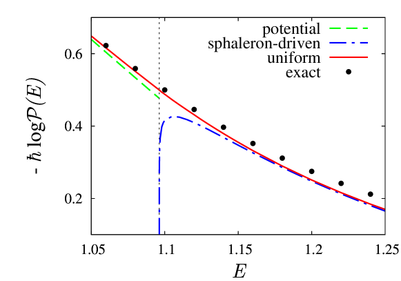
Figure 7: Uniform approximation for the tunneling probability (solid line) shown at $\hbar=1/30$, $E_{y}=0.05$ in the vicinity of the critical energy $E_{c}(E_{y})\approx 1.1$. We also plot the semiclassical results of Secs. 4.1 and 4.2 (dashed lines) and exact quantum probability (points). The critical energy is marked with the vertical dotted line.

To summarize, we derived the continuous asymptotic formula for the tunneling probability, Eq. (23), which works at energies close to critical and interpolates between the two semiclassical expressions corresponding to the cases of potential and sphaleron–driven tunneling. In Fig. 7 we compare the uniform approximation (23) (solid line) with the semiclassical probabilities ${\cal P}_{pot}$ and ${\cal P}_{sph}$ (dashed lines), as well as with the exact quantum probability (points).

5 Exclusive processes

Here we study semiclassically the effect of the new tunneling mechanism on exclusive processes, i.e. processes with completely fixed out-states. We discuss the application of the modified semiclassical technique to the exclusive case and obtain expressions, analogous to Eqs. (22), for the suppression exponent and prefactor of exclusive probability. We show that in the semiclassical limit of vanishingly small $\hbar$ the exclusive prefactor $A_{e,sph}$ is proportional to $\hbar^{2}$ in the sphaleron–driven case. This should be compared with the dependence $A_{e,pot}\propto\hbar$ in the case of potential tunneling.

5.1 Exclusive trajectories

We consider tunneling transitions between the exclusive states $|E,\,E_{y}\rangle$ and $|E,\,E_{y}^{f}\rangle$ specified by the same value of total energy $E$ and definite energies $E_{y}$, $E_{y}^{f}$ of $y$-oscillator. The standard semiclassical method in the case of exclusive transitions is formulated in Ref. [22]. Its derivation is completely analogous to that carried out in Sec. 4.1 for inclusive processes. Fixation of the out-state changes the final boundary conditions for the complex trajectory: instead of Eqs. (8) one has,

$$x_{f}=x_{f}^{(0)}\;,\qquad\qquad E_{y}^{f}=(\dot{y}_{f}^{2}+\omega^{2}y_{f}^{2})/2\;.$$ (29)

The initial conditions remain the same, Eqs. (5). The exclusive suppression exponent is given by the action functional

$$F_{e,pot}=2\mathrm{Im}(S[\boldsymbol{x}]+B_{i}[\boldsymbol{x}]-B_{f}[\boldsymbol{x}])\;,$$ (30)

computed on the trajectory, cf. Eq. (9). Note that the new term $B_{f}$ in Eq. (30) is related to the out–state of the process; it is given by the same expression as $B_{i}$, but at $t=t_{f}$ and with the out-state quantum numbers $E$, $E_{y}^{f}$. We do not write here the formula for the prefactor $A_{e,pot}$; it can be found in Ref. [22]. Importantly, this formula implies that $A_{e,pot}\propto\hbar$.

We apply the above method in the case of potential tunneling, $E<E_{c}(E_{y})$. In Fig. 8a (lines) we plot the out–state distributions of the exclusive exponent (30) for several values of energy $E$. The exact results (points) are extracted from the fit (13) with $\gamma=1$. The semiclassical and exact data coincide.

One observes that well below the critical energy $E_{c}(E_{y})\approx 1.1$ the function $F_{e,pot}(E_{y}^{f})$ has a clear minimum corresponding to a sharp maximum of the quantum probability. As the energy tends to $E_{c}(E_{y})$, a flat plateau develops in the right side of the graph. As discussed in Sec. 3, this behavior is copied by the exact quantum probability, cf. Fig. 4a.

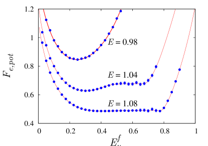
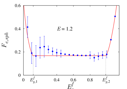
(a)                                                                     (b)

Figure 8: Exclusive suppression exponent $F_{e}$ in the cases of (a) potential and (b) sphaleron–driven tunneling; $E_{y}=0.05$. The semiclassical results for $F_{e}$ (lines) are compared with the exact data (points). Errorbars represent the uncertainty of the fit (13).

Before introducing the semiclassical method for exclusive tunneling in the sphaleron–driven case, we preview the result for the suppression exponent $F_{e,sph}$ in Fig. 8b (solid line). At $E>E_{c}(E_{y})$ the exclusive exponent is exactly constant in the region $E_{y,1}^{f}<E_{y}^{f}<E_{y,2}^{f}$; clearly, this feature corresponds to a wide and flat maximum of quantum probability, cf. the exact graphs in Fig. 4b. Thus, the distribution of the exclusive probability over the out-state quantum numbers becomes anomalously wide when the sphaleron–driven mechanism is involved. So far the semiclassical study of this property was restricted to one–dimensional systems with non–autonomous potentials [25, 30]. Here we find the same effect in the two–dimensional setup of Sec. 2.

Returning to the semiclassical description of exclusive tunneling processes, we find the following manifestation of the sphaleron–driven mechanism. In contrast to the case of potential tunneling where the exclusive trajectory is unique, at $E>E_{c}(E_{y})$ there is an infinite sequence of complex trajectories corresponding to the same final oscillator energy $E_{y}^{f}$. In Fig. 9 we plot the first four trajectories for $E_{y}^{f}=0.6$.

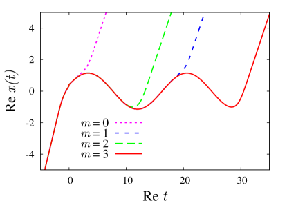
Figure 9: Four exclusive trajectories at $E_{y}^{f}=0.6$. The initial parts of the trajectories are indistinguishable on the graph. The in-state quantum numbers are $E=1.2$, $E_{y}=0.05$.

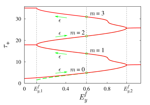
Figure 10: The curve in $(E_{y}^{f},\tau_{+})$–plane (solid line) representing exclusive tunneling trajectories. Circles correspond to the trajectories from Fig. 9. The dashed line represents the modified inclusive trajectories. It is almost coincident with the sin–like part of the solid line. Arrows indicate the direction of decreasing $\epsilon$. The in-state quantum numbers are the same as in Fig. 9.

One observes the following behavior: the trajectories reach the unstable periodic orbit (sphaleron), perform several oscillations there (i.e. around the point $x=0$) and then slide off describing the sphaleron decay into the final state. Importantly, in order to arrive into the out-state with given $E_{y}^{f}$, the trajectory must leave the sphaleron at a particular oscillation phase $\varphi$. More precisely, there are two choices of phase per sphaleron period. We conclude that the interaction time $\tau_{+}$ spent by the exclusive tunneling trajectories at given $E_{y}^{f}$ is restricted to two values plus an integer number of sphaleron periods. This gives rise to an infinite family of tunneling trajectories which describe the same exclusive process but differ by the number of “half–period” oscillations on top of the unstable periodic orbit.

To investigate the properties of exclusive trajectories in the sphaleron–driven case, we proceed as follows. For each trajectory we compute the value of the interaction time functional $\tau_{+}=\mathrm{Re}\,T_{int}[\boldsymbol{x}]$, Eq. (14). In this way we characterize the trajectories by points in the plane $(E_{y}^{f},\tau_{+})$, see Fig. 10.

A comment is in order. The exclusive tunneling trajectories are stable even in the sphaleron–driven case. Thus, they can be found without $\epsilon$–regularization. Still, as we will discuss shortly, it is convenient to use the modified semiclassical technique at the intermediate steps of the computation and remove the regularization afterwards. To avoid confusion, let us stress that the solid line in Fig. 10 corresponds to trajectories which are obtained after removal of the regularization. Consequently, the functional $T_{int}[\boldsymbol{x}]$ does not enter the equations of motion for these trajectories and is used only to characterize their temporal behavior.

From Fig. 10 one sees that the exclusive trajectories are naturally divided into two classes. The trajectories from the first class lie in the interval $E_{y,1}^{f}<E_{y}^{f}<E_{y,2}^{f}$ corresponding to the plateau in Fig. 8b. In Fig. 10 they form a sin–like curve extended to the infinite values of $\tau_{+}$. All these trajectories describe creation and subsequent decay of the sphaleron. Moreover, we find that the latter decay proceeds classically since the imaginary part of the trajectories becomes small after one sphaleron oscillation. As a consequence, the value of the functional (30) is almost independent of the individual trajectory from the first class. Besides, it is clear from the figure that these trajectories form an infinite sequence of branches marked with the integer number $m$ of “half–period” oscillations in the vicinity of the sphaleron.

The trajectories from the second class represent the “wings” $E_{y}^{f}<E_{y,1}^{f}$, $E_{y}^{f}>E_{y,2}^{f}$ of the out-state distribution in Fig. 8b. They correspond to the case when the decay of the sphaleron orbit into the out-state with given $E_{y}^{f}$ cannot proceed classically. Consequently, the probability of this decay is exponentially suppressed. Due to the additional suppression, the exponent (30) strongly depends on the out-state at $E_{y}^{f}<E_{y,1}^{f}$, $E_{y}^{f}>E_{y,2}^{f}$. Note, however, that the sphaleron still serves as the mediator of the two-stage tunneling process; hence, the second–class trajectories with fixed $E_{y}^{f}$ form an infinite sequence marked with the topological number $m$, see Fig. 10. The values of the suppression exponents $F_{e,pot}^{(m)}$ calculated on trajectories with different topology and given $E_{y}^{f}$ are almost degenerate.

In practice the exclusive trajectories are conveniently found using the regularization method of Sec. 4.2. The procedure is based on the following observation. Consider $\epsilon$–regularized trajectories corresponding to the inclusive tunneling process. They describe creation and subsequent classical decay of the sphaleron. The final state of the decay depends on the value of $\epsilon$. Changing $\epsilon$ one covers the whole range of final oscillator energies $E_{y,1}^{f}\leq E_{y}^{f}\leq E_{y,2}^{f}$ accessible in the classical sphaleron decay. This consideration is illustrated by the dashed curve in Fig. 10 which represents the modified inclusive trajectories at different values of $\epsilon$ in the $(E_{y}^{f},\tau_{+})$ – plane. We see that the graph closely follows the sin–like curve of exclusive trajectories from the first class, and the value of $\epsilon$ decreases towards large $\tau_{+}$ (along arrows). Thus, the modified solutions with different $\epsilon$ form a single branch which smoothly interpolates between the branches of exclusive trajectories.

Numerically, we exploit the above property by applying the deformation procedure of appendix B. Namely, we start with the modified trajectory at a given $E_{y}^{f}=E_{y,0}^{f}$. Suppose it has topology $m$. Then, the trajectory with topology $m+1$ ($m-1$) is obtained by decreasing (increasing) the value of $\epsilon$ until the final oscillator energy arrives to $E_{y,0}^{f}$ again (see Fig. 10). Repeating this procedure, we find the sequence of modified trajectories at $E_{y}^{f}=E_{y,0}^{f}$. Finally, we impose the boundary conditions (29) and set $\epsilon=0$. In this way we find all exclusive trajectories from the first class sorted by the topological number $m$. The solutions at the “wings” are obtained by taking the trajectories corresponding to $E_{y}^{f}=E_{y,1}^{f}$ ($E_{y,2}^{f}$) and deforming them by decreasing (increasing) $E_{y}^{f}$.

5.2 Exclusive probability

Let us derive the expression of the form (1) for the exclusive tunneling probability in the sphaleron–driven case. We start with the semiclassical formula

$${\cal P}_{e}=\sum_{m=0}^{\infty}A_{e,pot}^{(m)}\cdot\mathrm{e}^{-F_{e,pot}^{(m)}/\hbar}\;,$$ (31)

where the sum runs over all complex trajectories describing the same process. Note that the terms due to interference between different trajectories are neglected in Eq. (31); we will discuss them later. One recalls that the number $m$ of exclusive trajectory increases with the time interval $\tau_{+}$ spent by the trajectory in the vicinity of the sphaleron orbit. In accordance with the new tunneling mechanism this implies that the sum in Eq. (31) is saturated at $m\to+\infty$: the individual suppressions $F_{e,pot}^{(m)}$ decrease with $m$ and reach the minimum at $m\to+\infty$. This minimum is the overall suppression exponent of the process,

$$F_{e,sph}=\lim_{m\to+\infty}F_{e,pot}^{(m)}\;.$$ (32)

Note that the value of $F_{e,sph}$ is the same for all trajectories from the first class and equal to the suppression $F_{sph}$ of inclusive tunneling probability. This property gives rise to the plateau in the dependence $F_{e,sph}(E_{y}^{f})$ in Fig. 8b.

Let us now turn to the prefactor. Since the suppressions $F_{e,pot}^{(m)}$ change at large $m$ in small steps, one may be tempted to replace the sum in Eq. (31) by the integral and evaluate it in a straightforward way. However, this replacement is in general incorrect: even for small change of $F_{e,pot}^{(m)}$ the change in the exponent ${\rm e}^{-F_{e,pot}^{(m)}/\hbar}$ can be large.

We proceed carefully. In what follows we restrict our attention to the plateau case $E_{y,1}^{f}<E_{y}^{f}<E_{y,2}^{f}$. One starts by relating the limit $m\to+\infty$ of exclusive quantities to $A_{sph}$,

$$\lim_{m\to+\infty}A_{e,pot}^{(m)}\left|\frac{dF_{e,pot}^{(m)}}{dE_{y}^{f}}\right|^{-1}=\omega A_{sph}\;.$$ (33)

This formula is obtained as follows. One changes the integration variables from $\tau_{+}$ to $E_{y}^{f}$ in the expression (20) for inclusive probability,

$$\int d\tau_{+}=\int dE_{y}^{f}\sum_{m}\left|\frac{d\tau_{+}}{dE_{y}^{f}}\right|\;,$$

where the derivative is taken along the dashed line in Fig. 10. Comparing the resulting integral with the relation

$${\cal P}=\int\frac{dE_{y}^{f}}{\hbar\omega}\,{\cal P}_{e}$$

between the inclusive and exclusive probabilities, one expresses the modified suppression exponent and prefactor in terms of $F_{e,pot}^{(m)}$, $A_{e,pot}^{(m)}$,

$$F_{\epsilon}=F_{e,pot}^{(m)}\;,\qquad\qquad A_{pot,\epsilon}=A_{e,pot}^{(m)}\cdot\frac{\sqrt{\pi}}{\omega\sqrt{\hbar}}\left[-\frac{d\tau_{+}}{d\epsilon}\right]^{1/2}\left|\frac{dE_{y}^{f}}{d\tau_{+}}\right|\;.$$ (34)

Note that the value of $\epsilon$ in these formulas is fixed by the specification of the final oscillator energy $E_{y}^{f}$ and topological number $m$ of the respective trajectory. Now, one notes that the limit in Eq. (22b) can be computed by considering the subclass of modified trajectories with fixed $E_{y}^{f}$. These are close to the respective exclusive solutions; one uses the latter in the r.h.s. of Eq. (22b) and substitutes the limit $\epsilon\to+0$ with $m\to+\infty$. Then, Eqs. (34) and the Legendre transformation (21) imply Eq. (33).

Now, we exploit the dependence of the individual suppressions $F_{e,pot}^{(m)}$ on $m$ at large $m$. It is shown in appendix D that the suppressions approach the limiting value $F_{sph}$ exponentially,

$$F_{e,pot}^{(m)}-F_{sph}=\begin{cases}\alpha_{even}(E_{y}^{f})\,{\rm e}^{-\beta n}~{},&m=2n\\ \alpha_{odd}(E_{y}^{f})\,{\rm e}^{-\beta n}~{}~{},&m=2n+1\end{cases}$$ (35)

where the coefficient $\beta=\tilde{\beta}T_{sph}$ is related to the positive Lyapunov exponent $\tilde{\beta}$ and period $T_{sph}$ of the sphaleron orbit. Clearly, $\beta$ does not depend on the final oscillator energy. Substituting Eqs. (35), (33) into the formula (31), we find,

$$\begin{split}{\cal P}_{e}={\rm e}^{-F_{sph}/\hbar}\cdot\omega A_{sph}\bigg{\{}&\left|\frac{d\alpha_{even}}{dE_{y}^{f}}\right|\sum_{n=0}^{\infty}\exp\left(-\beta n-\frac{\alpha_{even}}{\hbar}{\rm e}^{-\beta n}\right)\\ &+\left|\frac{d\alpha_{odd}}{dE_{y}^{f}}\right|\sum_{n=0}^{\infty}\exp\left(-\beta n-\frac{\alpha_{odd}}{\hbar}{\rm e}^{-\beta n}\right)\bigg{\}}\;.\end{split}$$ (36)

Let us concentrate on the first term in braces, the second term is treated in the same way. The sum is saturated near the point $n_{0}$ corresponding to the maximum of the exponent,

$$n_{0}=-\frac{1}{\beta}\log\frac{\hbar}{\alpha_{even}}\;.$$ (37)

Generically, $n_{0}$ is not integer. Factoring out the value of the summand at $n=n_{0}$, one writes,

$$\sum_{n=0}^{\infty}\exp\left(-\beta n-\frac{\alpha_{even}}{\hbar}{\rm e}^{-\beta n}\right)=\frac{\hbar}{\alpha_{even}}\sum_{n=-\infty}^{\infty}\exp\left(-\beta(n-n_{0})-{\rm e}^{-\beta(n-n_{0})}\right)\;,$$ (38)

where in the r.h.s. we extended the sum to all integer $n$ by noting that the terms at $n<0$ are negligibly small. Substituting this relation into Eq. (36), one finally obtains expression for the exclusive prefactor,

$$A_{e,sph}=\hbar\omega A_{sph}\bigg{\{}\frac{1}{\alpha_{even}}\left|\frac{d\alpha_{even}}{dE_{y}^{f}}\right|~{}s\Big{(}\beta,\log{\frac{\hbar}{\alpha_{even}}}\Big{)}+\frac{1}{\alpha_{odd}}\left|\frac{d\alpha_{odd}}{dE_{y}^{f}}\right|~{}s\Big{(}\beta,\log{\frac{\hbar}{\alpha_{odd}}}\Big{)}\bigg{\}}\;,$$ (39)

where

$$s(\beta,\xi)\equiv\sum_{n=-\infty}^{\infty}\exp\left(-\beta n-\xi-{\rm e}^{-\beta n-\xi}\right)$$ (40)

is a periodic function of $\xi$ with period $\beta$.

Let us discuss our result. The dependence of the exclusive prefactor (39) on $\hbar$ is different in the cases $\beta\ll 1$, $\beta\sim 1$, $\beta\gg 1$. At $\beta\ll 1$ the sum in Eq. (40) can be replaced by the integral and one obtains $s(\beta,\xi)\approx 1/\beta$. Then the $\hbar$–dependence of $A_{e,sph}$ reduces to the simple proportionality law $A_{e,sph}\propto\hbar^{2}$. In the generic case $\beta\sim 1$ one observes, besides the overall scaling $A_{e,sph}\propto\hbar^{2}$, the modulation of the prefactor by the periodic function of $\log\hbar$. The latter modulation is elusive, however, in models with $\beta\gg 1$. Namely, the periodic nature of $s(\beta,\xi)$ becomes apparent only at $|\xi|=|\log(\hbar/\alpha_{even})|\sim\beta$ which corresponds to exponentially small values of $\hbar\sim\mathrm{e}^{-\beta}$.

Realistically, at large $\beta$ one works in the regime $\beta\gg|\xi|$. In this case the formulas (32), (39) are not applicable, since they are derived under the assumption $n_{0}\gtrsim 1$, see Eq. (37). At $n_{0}\ll 1$ one uses the original expression (31), where the sums over even/odd $m$ are saturated by the first terms. Then $A_{e,sph}\propto\hbar$. Let us roughly estimate the relative size of the terms with $m=0$ and $m=1$. One takes

$$F_{e,pot}^{(1)}-F_{sph}=\mathrm{e^{-c\beta}}(F_{e,pot}^{(0)}-F_{sph})\;,$$

where $c$ is a coefficient of order $1$, and uses Eq. (33) to estimate the prefactors. This yields that the trajectory with $m=1$ is relevant when

$$\hbar\lesssim\frac{F_{e,pot}^{(0)}-F_{sph}}{c\beta}$$ (41)

and is negligible at larger $\hbar$. One concludes that, depending on the value of $\hbar$, the term with $m=0$ or $m=1$ dominates.

The characteristic values of the parameter $\beta$ are related to the properties of the unstable periodic orbits, which are fixed in the model under consideration. As estimated in appendix D, in the setup (2) $\beta\sim 24$. On the other hand, the numerical quantum mechanical computations are feasible only down to $\hbar\gtrsim 10^{-2}$. Thus, we are in the regime $\hbar\gg\mathrm{e}^{-\beta}$, where the exclusive probability is saturated by the trajectories with $m=0,1$.

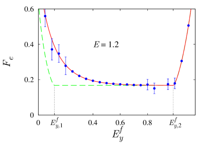
Figure 11: Exclusive suppression exponents in the sphaleron–driven case: the first exponent $F_{e,pot}^{(0)}$ (line), the limiting value $F_{e,sph}$ (dashed line) and the fit of the exact data with $\hbar\geq 1/120$ (errorbars). The in–state quantum numbers are the same as in Figs. 8b, 4b.

To see this explicitly, we compare the first suppression exponent $F_{e,pot}^{(0)}$ and the limiting exponent $F_{e,sph}$ with the exact suppression. Since in our case $A_{e,sph}\propto\hbar$, one extracts the exact suppression from the fit (13) with $\gamma=1$. We consider separately the exact data with $\hbar\geq 1/120$ and $\hbar<1/120$. Using the first set of data, we obtain the points in Fig. 11. The results of the fit closely follow $F_{e,pot}^{(0)}$ and differ substantially from the limiting exponent $F_{e,sph}$ in the left part of the graph. One concludes that at $\hbar\geq 1/120$ the trajectory with $m=0$ saturates the tunneling probability.

Second, we analyze the exact quantum data with $\hbar<1/120$. Consider Fig. 4b where the logarithm of the exact tunneling probability is plotted at several values of $\hbar$. One sees that the graph at $\hbar=1/140$ is notably different from the graphs at larger $\hbar$. We attribute this difference to the contribution of the trajectory with $m=1$. Indeed, at $E_{y}^{f}\approx E_{y,1}^{f}$ the difference in the suppressions is large, $F_{e,pot}^{(0)}-F_{e,sph}\sim 0.2$. Then, the estimate (41) implies that at $\hbar\lesssim 1/120$ the first odd trajectory enters into the game. The results of the fit of exact data with small $\hbar$ are shown in Fig. 8b. As expected, they coincide with $F_{e,sph}$ in the leftmost part of the graph.

Finally, let us briefly discuss interference between exclusive trajectories. Consider first the case $\beta\sim 1$. The sum (40) for the prefactor is then saturated by the fixed number of terms, $\Delta n=O(\hbar^{0})$. Since each term corresponds to the complex trajectory, the number of trajectories giving substantial contribution into the probability is finite, and the interference between the trajectories is important. This gives rise to oscillations in the dependence of the probability on the in– and out–state quantum numbers $E$, $E_{y}$, $E_{y}^{f}$. The period of these oscillations tends to zero as $\hbar\to 0$; thus, they become indiscernible in the semiclassical limit. However, at finite $\hbar$ the interference is important.

In our case of large $\beta$ the exclusive probability is dominated by two complex trajectories, and the interference picture is seen whenever the contributions of these trajectories are comparable. In accordance with the above discussion, this happens at $\hbar\sim 1/140$ and $E_{y}^{f}\approx E_{y,1}^{f}$, see Fig. 4b. The small–scale oscillations in the right part of the plateau in Fig. 4b are explained as follows. Let us take a look at Fig. 10. One observes that at $E_{y}^{f}\approx E_{y,2}^{f}$ the trajectory with $m=1$ is almost coincident with the dominant one. Thus, this trajectory gives substantial contribution into the probability in the vicinity of $E_{y,2}^{f}$, and the interference between the two trajectories is seen in this region.

6 The limit of small quantum numbers

According to the common lore low–lying quantum states are “not semiclassical.” Indeed, one cannot use the semiclassical expressions for the wave functions of these states in the majority of applications: at $E\sim\hbar$ the momentum is parametrically small and the semiclassical approximation is not justified. One finds, however, that tunneling processes are very special in regard of low–lying states. Namely, the semiclassical tunneling probability depends only on exponentially small tails of in- and out-state wave functions; these tails can be computed semiclassically even at small values of respective quantum numbers.

In this section we generalize the semiclassical method to the case of tunneling from the low–lying in-states of $y$-oscillator, $E_{y}\sim\hbar$. At the same time the total energy is assumed to be semiclassically large, $E\sim 1$. To be concrete, we take $E_{y}=\hbar\omega/2$, which corresponds to the oscillator ground state. Note, however, that the method of this section can be used for other low–lying oscillator states as well.

Let us address the following questions:
(i) Is it legitimate to use the semiclassical approximation for the wave function of the oscillator deep inside the classically forbidden region, $|y|\gg\hbar^{1/2}$ ?
(ii) Is the integral over initial states in Eq. (4) saturated deep inside the classically forbidden region at small $E_{y}$?
If the answers to the above questions are positive, one can use the semiclassical expressions for the probability of tunneling from the ground state of $y$-oscillator (e.g. Eqs. (9), (11) in the case of potential tunneling).

To answer the first question, we compare the semiclassical and exact oscillator wave functions in the case of ground state, $E_{y}=\hbar\omega/2$:

$$\psi_{y,s}(y) =\left(\frac{\omega}{2\pi p_{y,i}(y)}\right)^{1/2}\cdot\mathrm{exp}\left(\frac{i}{\hbar}\int_{\sqrt{2E_{y}}/\omega}^{y}p_{y,i}(y^{\prime})\,dy^{\prime}+\frac{i\pi}{4}\right)\;,$$ (42)

$$\psi_{y,0}(y) ={\left(\frac{\omega}{\pi\hbar}\right)}^{1/4}\cdot\mathrm{exp}\left(-\omega y^{2}/2\hbar\right)\;.$$ (43)

In the above expressions $|y|$ is large and $p_{y,i}(y)=\sqrt{2E_{y}-\omega^{2}y^{2}}$. Equations (42) and (43) look quite different: the exact wave function involves the factor $\hbar^{-1/4}$ which is not present in the semiclassical expression. However, substituting $E_{y}=\hbar\omega/2$ into the leading exponent of Eq. (42), one finds,

$$\int_{\sqrt{\hbar/\omega}}^{y}dy^{\prime}p_{i}(y^{\prime})=i\omega y^{2}/2-i\hbar/4-i\hbar/2\,\log\left(2y\sqrt{{\omega}/{\hbar}}\right)+O(\hbar^{2})\;.$$

Thus, up to high–order semiclassical corrections

$$\psi_{y,0}(y)=\left(\frac{\pi}{\mathrm{e}}\right)^{1/4}\cdot\psi_{y,s}(y)\Big{|}_{E_{y}=\hbar\omega/2}\;.$$ (44)

One concludes that the two wave functions are related by the simple renormalization factor $(\pi/\mathrm{e})^{1/4}$.

The relation (44) is not surprising. Indeed, the standard derivation of the semiclassical wave function (42) proceeds in two steps. First, one solves the Schrödinger equation with $\psi_{y,s}(y)=C\cdot\mathrm{e}^{i\sigma(y)/\hbar}$ considering $\sigma/\hbar\gg 1$. This is certainly valid deep inside the classically forbidden region, even for $E_{y}=\hbar\omega/2$. The second step is the evaluation of the normalization constant $C$ by taking the integral $\int|\psi_{y,s}(y^{\prime})|^{2}dy^{\prime}=1$. At small $E_{y}$ the latter integral is saturated at $y\approx 0$, i.e. right in the vicinity of the turning points, where the semiclassical expression (42) is not applicable. Consequently, the semiclassical calculation produces an incorrect value for the constant $C$ at $E_{y}=\hbar\omega/2$. Equation (44) shows that the correct value is $(\pi/e)^{1/4}$ times larger than the one obtained semiclassically.

We have the following answer to the question (i): the semiclassical expression (10) can be used at $E_{y}=\hbar\omega/2$ deep inside the classically forbidden region; however, the final result for the probability should be multiplied by the correction factor $(\pi/\mathrm{e})^{1/2}$.

Let us address the question (ii). Consider the complex trajectory $\boldsymbol{x}(t)$ in the in-region. One finds,

$$x(t)\to p_{x,i}(t-t_{i})+x_{i}\;,\qquad y(t)\to a\mathrm{e}^{-i\omega t}+\bar{a}\mathrm{e}^{i\omega t}\qquad\mbox{as}\qquad t\to-\infty\;.$$ (45)

The initial boundary conditions (5) guarantee that the quantities $p_{x,i}=\sqrt{2(E-E_{y})}$ and $a\bar{a}=E_{y}/2\omega^{2}$ are real. Therefore, one can define two real parameters $T$, $\theta$ by the relations

$$\mathrm{Im}\,x_{i}=-p_{x,i}T\;,\qquad a^{*}=\bar{a}\mathrm{e}^{-2\omega T-\theta}\;.$$ (46)

As discussed in Refs. [38, 26], these parameters are in one-to-one correspondence with the in-state quantum numbers $E$, $E_{y}$. In other words, $T$ and $\theta$ provide an alternative parameterization of tunneling trajectories. Note that $T=\theta=0$ represent classically allowed transitions, $\boldsymbol{x}(t)\in\mathbb{R}$. On the other hand, the limit $\theta\to+\infty$ corresponds to $E_{y}\to 0$. Indeed, in this limit one obtains $a\to 0$ and $\bar{a}$ finite [38, 26], which are the Feynman boundary conditions for tunneling from the ground state. From Eq. (45) one finds that $|y_{i}|\to|\bar{a}|\gg\hbar^{1/2}$. Thus, the integral over initial states in Eq. (4) is saturated deep inside the classically forbidden region, where the semiclassical expression for the in-state wave function is trustworthy.

One concludes that, apart from the additional multiplier $(\pi/\mathrm{e})^{1/2}$, the semiclassical expressions for the tunneling probability (1), such as Eqs. (9), (11), are still applicable at $E_{y}=\hbar\omega/2$.

Note that in the considered case of tunneling from the ground state the expressions (9), (11) depend on $\hbar$ in non-trivial way through $E_{y}=\hbar\omega/2$. It is convenient to extract this dependence explicitly and bring the expression for the tunneling probability into the form (1) with $F$ independent of $\hbar$ and $A$ having only the power-law dependence. This is done in appendix F, the result is

$$F_{pot,0}=\lim_{E_{y}\to+0}F_{pot}\;,\qquad A_{pot,0}=\left(\pi/\hbar\right)^{1/2}\,\mathrm{e}^{\theta_{0}/2}\lim_{E_{y}\to+0}A_{pot}\;.$$ (47)

where $F_{pot}$ and $A_{pot}$ are the standard semiclassical expressions for the suppression exponent and prefactor. The quantity $\theta_{0}$ entering Eq. (47) is extracted from the small–$E_{y}$ asymptotic of the leading exponent

$$F_{pot}=F_{pot,0}+\frac{E_{y}}{\omega}\log(2E_{y}/\omega)-\frac{\theta_{0}+1}{\omega}E_{y}+O(E_{y}^{2})\;.$$ (48)

Let us remark on Eqs. (47). First, note that $A_{pot,0}$ contains the additional factor $\hbar^{-1/2}$ as compared to the case of highly excited in-states. Second, we did not use the dynamical properties of complex trajectories in the derivation of Eqs. (47). Thus, the above expressions are valid both for inclusive and exclusive processes. They also hold in the case of sphaleron–driven tunneling, where one substitutes $F_{pot}\to F_{sph}$, $A_{pot}\to A_{sph}$ in Eqs. (47). In particular, for the prefactors of inclusive processes one has $A_{pot,0}\propto\hbar^{0}$ and $A_{sph,0}\propto\hbar^{1/2}$.

    

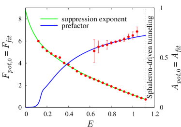
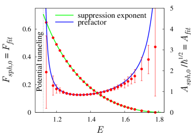
(a)                                                                   (b)

Figure 12: Comparison between the exact (points) and semiclassical (lines) results for the suppression exponent and prefactor at $E_{y}=\hbar\omega/2$ in the cases of (a) potential and (b) sphaleron–driven tunneling. Note that $E_{c}(0)\approx 1.1$. Errorbars represent uncertainty of the fit (13).

Finally, it is worth mentioning that the first of Eqs. (47), namely, the limiting relation between the suppression exponents of tunneling from the low–lying and highly excited in-states is known in field theory as the Rubakov–Son–Tinyakov conjecture [36]. We proved this conjecture in quantum mechanical setup.

We close this section by comparing the semiclassical results for the suppression exponent and prefactor, Eqs. (47), with the results extracted by the fit Eq. (13) from the solution of the Schrödinger equation. The comparison in the cases of potential and sphaleron–driven tunneling is presented in Figs. 12a, 12b for inclusive and in Figs. 13a, 13b for exclusive processes. In the latter case we compare the exact suppression exponent with the suppression of the first exclusive trajectory.

    

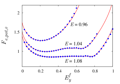
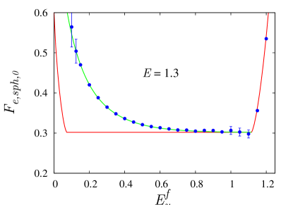
(a)                                                                       (b)

Figure 13: Comparison between the exact (points) and semiclassical (lines) results for the suppression exponent of exclusive processes at $E_{y}=\hbar\omega/2$ in the cases of (a) potential and (b) sphaleron–driven tunneling. In the case (b) the exact data coincide with the first exponent $F_{e,pot,0}^{(0)}$. Errorbars represent uncertainty of the fit (13).

One observes nice agreement.

7 Summary and Discussion

In this paper we investigated the mechanism of tunneling via unstable semiclassical solutions (sphaleron–driven tunneling) which governs the processes of multidimensional tunneling at energies higher than some critical value $E_{c}$. There were two aspects in our study. First, we analyzed the experimental signatures of sphaleron–driven tunneling. These are suppression of the tunneling probability by the additional power of the semiclassical parameter $\hbar$ and substantial widening of the final–state distributions as compared to the case of ordinary barrier tunneling.

The second aspect of this paper was related to the development of the modified semiclassical technique (the method of $\epsilon$–regularization), which is applicable in the case of sphaleron–driven tunneling. This method is completely general; it was derived from first principles using the formal operations with the path integral. Similar modified technique has been implemented in several quantum mechanical [26, 16] and field theoretical [32] tunneling problems. Using the modified method, we obtained expressions for the inclusive and exclusive tunneling probabilities in the case of sphaleron–driven mechanism, investigated the “phase transition” between the cases of potential and sphaleron–driven tunneling. We also derived relation between the probabilities of tunneling from the low–lying and highly excited in-states.

Our results for the power–law dependences of the semiclassical prefactor are summarized in Table 1.

Potential Sphaleron–driven Inclusive, $E_{y}\sim 1$ $\hbar^{1/2}$ $\hbar$ Exclusive, $E_{y}\sim 1$ $\hbar$ $\hbar^{2}$ Inclusive, $E_{y}\sim\hbar$ $\hbar^{0}$ $\hbar^{1/2}$ Exclusive, $E_{y}\sim\hbar$ $\hbar^{1/2}$ $\hbar^{3/2}$

Table 1: Summary: the power–law dependences of the tunneling probability in two dimensions.

Let us comment on the relation between the mechanism of sphaleron–driven tunneling and Wilkinson formula for the tunnel energy splitting [6, 7, 8, 9]. The latter formula is applicable in the cases of near–integrable (as opposed to completely integrable) systems with double–well potentials. It is based on the following property of near–integrable dynamics: tunneling trajectories stemming from the wells of near–integrable system do not end up in opposite wells (as in the integrable case), but rather get attracted to a certain unstable periodic orbit. Due to this feature the splitting in Wilkinson formula is suppressed by the additional factor $\hbar^{1/2}$ as compared to the case of completely integrable system. One observes that, technically, the reason for this factor is similar to that in the mechanism of sphaleron–driven tunneling considered in this paper. However, the two cases are physically different: transition to the sphaleron–driven regime is unrelated to the transition from integrable to non–integrable dynamics. In addition, the relevant periodic orbit in the Wilkinson formula is complex while the sphaleron orbit is real.

We finish this paper with remarks on the recent observation [29] that the new tunneling mechanism generically leads to anomalously large times of tunneling. Indeed, the semiclassical trajectories describing sphaleron–driven transitions spend infinite time interval in the vicinity of the sphaleron orbit. Clearly, the time scale $\Delta t$ of such transitions should be large, in particular, one expects $\Delta t\to+\infty$ as $\hbar\to 0$. A rough estimate of $\Delta t$ can be obtained as follows. Due to quantum fluctuations the system cannot approach the sphaleron orbit in the phase space closer than at the distance determined by the uncertainty principle, $\Delta\boldsymbol{p}\Delta\boldsymbol{x}\sim\hbar$. The semiclassical trajectories starting in the vicinity of unstable sphaleron go away from it exponentially with time; thus it takes them the time $\Delta t\sim\log|\Delta\boldsymbol{p}|,\log|\Delta\boldsymbol{x}|$ to leave the sphaleron neighborhood. This translates into the characteristic lifetime of the sphaleron $\Delta t\propto|\log\hbar|$, which sets the characteristic time scale for sphaleron–driven tunneling. The dependence of tunneling time on $\hbar$ provides another possible experimental signature of the new tunneling mechanism. Yet more signatures can be found by analyzing the probability distribution over tunneling time. The modified semiclassical method proposed in this paper allows comprehensive study of these issues which will be published elsewhere [41].

Acknowledgments.

We are indebted to F.L. Bezrukov, S.V. Demidov, D.S. Gorbunov, M.V. Libanov, N.S. Manton, V.V. Nesvizhevsky and V.A. Rubakov for useful and stimulating discussions. This work was supported in part by the RFBR grant 08-02-00768-a, Grants of the President of Russian Federation NS-1616.2008.2 and MK-1712.2008.2 (D.L.), Grant of the Russian Science Support Foundation (A.P.), the Fellowships of the “Dynasty” Foundation (awarded by the Scientific board of ICPFM) (D.L. and A.P.) and the Tomalla Foundation (S.S.). The numerical calculations were performed on the Computational cluster of the Theoretical division of INR RAS.

Appendix A Semiclassical tunneling probability

In this appendix we give details of the standard method of complex trajectories. The main idea of the method is presented in Sec. 4.1.

Our starting point is the path integral representation (4) for the out-state wave function $\Psi_{f}$. This representation contains two main ingredients, the in-state $\Psi_{i}$ and the quantum propagator written as a path integral. In accordance with the discussion in the main body of the paper, the in-state has definite values of the total energy $E$ and $y$-oscillator energy $E_{y}$. One writes $\Psi_{i}(x,\,y)$ as a product $\psi_{x}(x)\cdot\psi_{y}(y)$, where $\psi_{x}$ is a plane wave with momentum $p_{x,i}=\sqrt{2(E-E_{y})}$ and unit flux normalization, while $\psi_{y}$ represents the semiclassical wave function of the oscillator with energy $E_{y}$. Combining $\psi_{x}$ and $\psi_{y}$, one obtains,

$$\Psi_{i}(x,y)=\left(\frac{\omega}{2\pi p_{y,i}(y)p_{x,i}}\right)^{1/2}\cdot\exp\left(\frac{i}{\hbar}B_{i}(x,y)+\frac{i\pi}{4}\right)\;.$$ (49)

In this formula $p_{y,i}(y)=\sqrt{2E_{y}-\omega^{2}y^{2}}$ is the $y$ component of the momentum in the in-region $x\to-\infty$, while

$$B_{i}(x,y)=p_{x,i}x+\int_{\sqrt{2E_{y}}/\omega}^{y}p_{y,i}(y^{\prime})\,dy^{\prime}$$ (50)

stands for the classical action in this region. Note that in Eq. (49) we keep only one of the two exponents entering the standard expression for the oscillator wave function. The reason is that $\Psi_{i}(x,y)$ will be used deep inside the classically forbidden region, where the omitted exponent is negligible.

At small $\hbar$ the path integral for the quantum propagator is evaluated by the saddle–point technique. The result is given by the Van Vleck formula [43, 22],

$$\left.\int[d\boldsymbol{x}]\right|_{\boldsymbol{x}_{i}}^{\boldsymbol{x}_{f}}\,\mathrm{e}^{iS[\boldsymbol{x}]/\hbar}=\frac{\mathrm{e}^{iS[\boldsymbol{x}^{(s)}]/\hbar}}{2\pi i\hbar}\cdot\left[\det\frac{\partial^{2}S}{\partial\boldsymbol{x}_{i}\partial\boldsymbol{x}_{f}}\right]^{1/2}\;.$$ (51)

We refer the interested reader to Ref. [44] for derivation. The formula (51) is written in terms of the semiclassical trajectory $\boldsymbol{x}^{(s)}(t)$, which has the meaning of a saddle–point path saturating the path integral. This trajectory satisfies the classical equations of motion; it starts from $\boldsymbol{x}=\boldsymbol{x}_{i}$ at $t=t_{i}$ and arrives to $\boldsymbol{x}=\boldsymbol{x}_{f}$ at $t=t_{f}$. Below we omit the superscript $(s)$ of the semiclassical trajectory.

We substitute the semiclassical expressions (49) and (51) into Eq. (4) and take the saddle–point integral over $\boldsymbol{x}_{i}$. The result for the out-state wave function has the exponential form (6), where $D^{-1/2}$ collects all prefactors including the determinant due to the saddle–point integration; we will evaluate $D$ below. Note that integration over $\boldsymbol{x}_{i}$ changes initial conditions for the trajectory $\boldsymbol{x}(t)$. Namely, the extremum of the leading exponent $S+B_{i}$ with respect to $\boldsymbol{x}_{i}$ is achieved when

$$\dot{x}_{i}=p_{x,i}\;,\qquad\qquad\dot{y}_{i}=p_{y,i}(y_{i})\;.$$ (52)

One finds that these conditions are equivalent to the fixation of the in-state quantum numbers, Eqs. (5).

A remark is in order. We consider the case of classically forbidden transitions which implies that there is no real solutions starting in the in-region with fixed $E$, $E_{y}$ and arriving into the out-region at $t=t_{f}$. Accordingly, the saddle–point trajectory $\boldsymbol{x}(t)$ is complex.

Given the final state wave function, one evaluates the inclusive probability of tunneling performing the saddle–point integration over $y_{f}$ in Eq. (7). One obtains the familiar semiclassical formula (1) for the inclusive tunneling probability, where the leading exponent $F_{pot}$ is given by the value of the action functional (9) evaluated on the complex trajectory $\boldsymbol{x}(t)$. The prefactor will be discussed shortly.

Let us comment on the final boundary conditions (8) obtained after integration over $y_{f}$. One finds that all of them have different origin. Namely, the final value of $x_{f}$ is already fixed in the probability formula (7); the condition $\dot{y}_{f}=\dot{y}_{f}^{*}$ corresponds to the extremum of the leading semiclassical exponent with respect to $y_{f}$. The third condition, namely, reality of $y_{f}$, follows from uniqueness of complex trajectory, which is assumed. One also notes that the trajectory $\boldsymbol{x}(t)$ is real in the out-region. Indeed, $x_{f}$, $y_{f}$, $\dot{y}_{f}$ are real due to the boundary conditions at $t=t_{f}$, while $\dot{x}_{f}\in\mathbb{R}$ due to conservation of total real energy $E$.

We finish the discussion of the complex trajectory $\boldsymbol{x}(t)$ by remarking shortly on the important issue of non–trivial contour in complex time [22, 38]. We noted already that $\boldsymbol{x}(t)$ is real in the out-region. Solving the classical equations of motion backwards in time, one concludes that at $t\in\mathbb{R}$ the trajectory is real as well. Thus, $\boldsymbol{x}(t)$ in real time corresponds to classically allowed reflection from the barrier; clearly this solution is not relevant for the description of tunneling. One observes, however, that the semiclassical trajectory has a branch point in the complex time plane, see Fig. 14. The solution describing tunneling is obtained along the contour winding around this branch point (the contour A’ABCD in the figure).

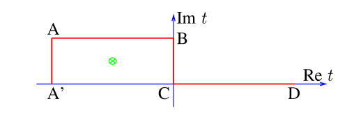
Figure 14: The tunneling solution is obtained along the contour $A^{\prime}ABCD$ in the complex time plane. The branch point of the solution is shown by the cross.

Let us evaluate the prefactor $A_{pot}$. There are two non–trivial contributions into $A_{pot}$ coming from the saddle–point integrations in Eqs. (4) and (7). We start with the prefactor $D^{-1/2}$ of the out-state wave function, Eq. (6). One finds that

$$D =\frac{2\pi}{\omega}\,\dot{y}_{i}\,\dot{x}_{i}\times(2\pi i\hbar)^{2}\left.\left[\det\frac{\partial\dot{\boldsymbol{x}}_{f}}{\partial\boldsymbol{x}_{i}}\right]^{-1}\times\frac{1}{(2\pi i\hbar)^{2}}\det{\frac{\partial^{2}(S+B_{i})}{\partial\boldsymbol{x}_{i}^{2}}}\right|_{\boldsymbol{x}_{f}=\mathrm{const}}$$

$$=\frac{2\pi}{\omega}\,\dot{y}_{i}\,\dot{x}_{i}\cdot\det\left.{\frac{\partial^{2}(S+B_{i})}{\partial\boldsymbol{x}_{i}\partial\dot{\boldsymbol{x}}_{f}}}\right|_{\boldsymbol{x}_{f}=\mathrm{const}},$$ (53)

where the three multipliers in the first line correspond respectively to the prefactors of the in-state (49), propagator (51) and the determinant due to the saddle–point integration over initial coordinates $\boldsymbol{x}_{i}$. In the second equality we combined the multipliers.

One substitutes the explicit form of $B_{i}$ into Eq. (53) and represents the factor $\dot{y}_{i}\,\dot{x}_{i}$ as the determinant of diagonal matrix. The result is

$$D=\frac{2\pi}{\omega}\left.\det\left[\begin{pmatrix}\dot{x}_{i}&0\\ 0&\dot{y}_{i}\end{pmatrix}\frac{\partial\dot{\boldsymbol{x}}_{i}}{\partial\dot{\boldsymbol{x}}_{f}}+\begin{pmatrix}0&0\\ 0&\omega^{2}y_{i}\end{pmatrix}\frac{\partial\boldsymbol{x}_{i}}{\partial\dot{\boldsymbol{x}}_{f}}\right]\right|_{\boldsymbol{x}_{f}=\mathrm{const}}\;.$$ (54)

This last determinant can be evaluated by considering the set of linear perturbations $\delta\boldsymbol{x}(t)$, which satisfy the linearized equation of motion (10) in the background of complex trajectory $\boldsymbol{x}(t)$. The two basic perturbations will be particularly important, $\boldsymbol{\psi}^{(1)}(t)=\partial\boldsymbol{x}(t)/\partial\dot{x}_{f}$ and $\boldsymbol{\psi}^{(2)}(t)=\partial\boldsymbol{x}(t)/\partial\dot{y}_{f}$, where the derivatives are taken at $\boldsymbol{x}_{f}=\mathrm{const}$. One can explicitly check that $\boldsymbol{\psi}^{(n)}(t)$ satisfy Eq. (10).

Consider linear energy increment due to perturbation $\delta\boldsymbol{x}(t)$,

$$\delta E[\delta\boldsymbol{x}]=\dot{x}_{i}\delta\dot{x}_{i}+\delta E_{y}[\delta\boldsymbol{x}]\;,$$ (55)

where the increment $\delta E_{y}[\delta\boldsymbol{x}]$ of the initial oscillator energy is given by Eq. (12). Clearly, $\delta E$ is conserved; in particular, it can be computed at $t=t_{f}$. Using the energy increments, one rewrites the determinant (54) as

$$D =\frac{2\pi}{\omega}\det\left[\begin{array}[]{cc}\delta E[\boldsymbol{\psi}^{(1)}]-\delta E_{y}[\boldsymbol{\psi}^{(1)}]&\delta E[\boldsymbol{\psi}^{(2)}]-\delta E_{y}[\boldsymbol{\psi}^{(2)}]\\ \delta E_{y}[\boldsymbol{\psi}^{(1)}]&\delta E_{y}[\boldsymbol{\psi}^{(2)}]\end{array}\right]$$ (58)

$$=\frac{2\pi}{\omega}\det\left[\begin{array}[]{cc}\dot{x}_{f}&\dot{y}_{f}\\ \delta E_{y}[\boldsymbol{\psi}^{(1)}]&\delta E_{y}[\boldsymbol{\psi}^{(2)}]\end{array}\right]$$ (61)

$$=\frac{2\pi}{\omega}\,\delta E_{y}[\dot{x}_{f}\boldsymbol{\psi}^{(2)}-\dot{y}_{f}\boldsymbol{\psi}^{(1)}]\;,$$

where in the last two equalities we added the second row to the first, computed explicitly $\delta E[\boldsymbol{\psi}^{(1)}]=\dot{x}_{f}$, $\delta E[\boldsymbol{\psi}^{(2)}]=\dot{y}_{f}$ and used linearity of $\delta E_{y}$. Let us introduce the linear combination

$$\delta\boldsymbol{x}^{(1)}(t)=-\dot{y}_{f}/\dot{x}_{f}\,\boldsymbol{\psi}^{(1)}(t)+\boldsymbol{\psi}^{(2)}(t)\;.$$

This vector satisfies the linearized equations of motion with the Cauchy data at $t=t_{f}$,

$$\delta\dot{\boldsymbol{x}}^{(1)}_{f}=(-\dot{y}_{f}/\dot{x}_{f},\;1)\;,\qquad\delta\boldsymbol{x}_{f}^{(1)}=0\;.$$ (62)

Note that $\delta E[\delta\boldsymbol{x}^{(1)}]=0$. Using $\delta\boldsymbol{x}^{(1)}$, one finds,

$$D=\frac{2\pi\dot{x}_{f}}{\omega}\,\delta E_{y}[\delta\boldsymbol{x}^{(1)}]\;.$$ (63)

So, we have obtained the final state prefactor $D^{-1/2}$ in Eq. (6).

Let us proceed with the probability prefactor $A_{pot}$. Taking the saddle–point integral in Eq. (7), one arrives at the following formula,

$$A_{pot}=\frac{\dot{x}_{f}\sqrt{\pi\hbar}}{|D|\sqrt{D^{\prime}}}\;,$$ (64)

where the factor coming from the integration is

$$D^{\prime}=\left.\mathrm{Im}\frac{\partial\dot{y}_{f}}{\partial y_{f}}\right|_{E,\,E_{y},\,x_{f}=\mathrm{const}}\;.$$ (65)

One evaluates $D^{\prime}$ considering the perturbation

$$\delta\boldsymbol{x}^{(2)}(t)=-\omega^{2}\frac{y_{f}}{\dot{x}_{f}}\,\boldsymbol{\psi}^{(1)}(t)+\left.\frac{\partial\boldsymbol{x}(t)}{\partial y_{f}}\right|_{\dot{\boldsymbol{x}}_{f},\,x_{f}=\mbox{\footnotesize const}}\;.$$

It satisfies the linearized equations of motion (10) with the final Cauchy data

$$\delta\dot{\boldsymbol{x}}^{(2)}_{f}=(-\omega^{2}y_{f}/\dot{x}_{f},\;0)\;,\qquad\delta\boldsymbol{x}^{(2)}_{f}=(0,\;1)\;,$$ (66)

so that $\delta E[\delta\boldsymbol{x}^{(2)}]=0$.

One notices that $\delta\boldsymbol{x}^{(1)}(t)$ and $\delta\boldsymbol{x}^{(2)}(t)$ do not change the values of $x_{f}$ and $E$. Moreover, these two are the only linearly independent perturbations which have this property. Thus, the perturbation

$$\boldsymbol{\rho}(t)=\left.\frac{\partial\boldsymbol{x}(t)}{\partial y_{f}}\right|_{E,\,E_{y},\,x_{f}=\mbox{\footnotesize const}}$$ (67)

is their linear combination, $\boldsymbol{\rho}(t)=\alpha\,\delta\boldsymbol{x}^{(1)}(t)+\beta\,\delta\boldsymbol{x}^{(2)}(t)$. One has,

$$\boldsymbol{\rho}_{y}(t_{f})=1 \Rightarrow \beta=1\;,$$

$$\delta E_{y}[\boldsymbol{\rho}]=\alpha\,\delta E_{y}[\delta\boldsymbol{x}^{(1)}]+\beta\,\delta E_{y}[\delta\boldsymbol{x}^{(2)}]=0 \Rightarrow \frac{\alpha}{\beta}=-\frac{\delta E_{y}[\delta\boldsymbol{x}^{(2)}]}{\delta E_{y}[\delta\boldsymbol{x}^{(1)}]}\;.$$

From Eqs. (65), (67) we deduce the formula

$$D^{\prime}=\mathrm{Im}\,\dot{\rho}_{y}(t_{f})=\mathrm{Im}\,{\alpha}=\frac{\mathrm{Im}\,\left(\delta E_{y}[\delta\boldsymbol{x}^{(1)}]\cdot\delta E_{y}^{*}[\delta\boldsymbol{x}^{(2)}]\right)}{|\delta E_{y}[\delta\boldsymbol{x}^{(1)}]|^{2}}\;.$$ (68)

Substituting expressions (63) and (68) into Eq. (64), one obtains Eq. (11).

We finally rewrite the Cauchy data (62), (66) for perturbations in canonically covariant form. The new conditions are:

(i) perturbations $\delta\boldsymbol{x}^{(n)}$ and their momenta $\delta\dot{\boldsymbol{x}}^{(n)}$ are real at $t=t_{f}$;

(ii) they do not perturb the total energy, $\delta E[\delta\boldsymbol{x}^{(n)}]=0$;

(iii) their norm is fixed by $\Omega(\delta\boldsymbol{x}^{(1)},\delta\boldsymbol{x}^{(2)})=1$, where $\Omega=dp_{x}\wedge dx+dp_{y}\wedge dy$ is the symplectic form.

Note that the conditions (i)—(iii) do not completely fix the perturbations $\delta\boldsymbol{x}^{(n)}$. Namely, a linear admixture of the perturbation $\boldsymbol{\chi}(t)=\dot{\boldsymbol{x}}(t)$, if added to $\delta\boldsymbol{x}^{(n)}$, does not disturb (i)—(iii) and the value of the prefactor $A_{pot}$. One shows this exploiting the properties of $\boldsymbol{\chi}$,

$$\delta E[\boldsymbol{\chi}]=\delta E_{y}[\boldsymbol{\chi}]=0\;,\qquad\qquad\Omega(\delta\boldsymbol{x}^{(1)},\boldsymbol{\chi})=\Omega(\delta\boldsymbol{x}^{(2)},\boldsymbol{\chi})=0\;.$$

In practice one fixes the $\boldsymbol{\chi}$–degeneracy by supplying some additional Cauchy datum.

It is straightforward to check that the conditions (i)—(iii) follow from Eqs. (62), (66). In fact, they are also sufficient, i.e. any pair of perturbations $\delta\boldsymbol{x}^{(1)}$ and $\delta\boldsymbol{x}^{(2)}$ satisfying (i)—(iii) can be used in the prefactor formula (11). One shows this explicitly by decomposing the new perturbations $\delta\boldsymbol{x}^{(n)}$ in the basis of the old perturbations, substituting them into Eq. (11) and using the properties (i)—(iii).

Let us note the following property of the formula (11) for $A_{pot}$. The perturbations $\delta\boldsymbol{x}^{(n)}(t)$ leave unchanged all boundary conditions of the complex trajectory except for one, fixation of $E_{y}$. It is precisely the change in this datum which enters the formula for the prefactor. In the limit of separable system, when $E_{y}$ becomes a conserved quantity, $\delta E_{y}[\delta\boldsymbol{x}^{(n)}]$ becomes real due to the condition (i) and $A_{pot}$ tends to infinity. This indicates the change of the $\hbar$-dependence of the prefactor in this limit, cf. Refs. [6, 8, 9].

Appendix B Numerical method for semiclassical calculations

Here we describe the numerical method of finding the trajectories $\boldsymbol{x}(t)$. The method has two useful properties. First, it is applicable to systems with arbitrary number of degrees of freedom, up to the field theory case (${\cal N}=\infty$). Second, it naturally incorporates the modified semiclassical technique of Sec. 4.2. Originally, the method was proposed in the field theoretical context [45, 32]. It was adapted for quantum mechanical problems in Ref. [38].

We compute $\boldsymbol{x}(t)$ by solving numerically the classical equations of motion with the boundary conditions (5) and (8) imposed at $t=t_{i}$ and $t=t_{f}$ respectively. To this end we introduce non–uniform lattice $\{t_{k},\;k=1\dots N_{k}\}$, where $t_{1}=t_{i}$, $t_{N_{k}}=t_{f}$, and discretize the classical equations of motion and boundary conditions in a straightforward manner. We find that the second–order discretization works well enough. As mentioned in appendix A, the time variable $t$ runs along the contour in complex time plane, see Fig. 14. Accordingly, the sites $t_{k}$ of the lattice belong to this contour.

After discretization one obtains the system of $2\times N_{k}$ complex non–linear algebraic equations for the same number of unknowns $\boldsymbol{x}_{k}=\boldsymbol{x}(t_{k})$. Let us denote the unknowns collectively by $z_{a}$, where $a=1\dots 2N_{k}$, and equations by ${\cal F}_{b}(z)=0$. We solve the equations by the Newton-Raphson iterative method, see e.g. Ref. [46]. In this method one starts with some approximation $z=z^{(0)}$ for the solution. Then the approximation is repeatedly refined by finding corrections $\Delta z$ from the system of linear equations

$${\cal F}_{a}(z^{(0)}+\Delta z)\approx\sum_{b}\frac{\partial{\cal F}_{a}}{\partial z_{b}}(z^{(0)})\,\Delta z_{b}+{\cal F}_{a}(z^{(0)})=0\;.$$

Note that the coefficient matrix of this system is block three–diagonal and can be inverted efficiently. At the end of each iteration one redefines the approximation, $z^{(0)}\to z^{(0)}+\Delta z$. After $3-6$ iterations the method converges provided the original approximation was good enough.

The drawback of the Newton–Raphson method is the small radius of convergence. Namely, the method does not produce correct solution unless the approximation $z^{(0)}$ is sufficiently close to it. We solve this difficulty in the following way. Suppose the solution is known for some values $(E,\,E_{y})$ of the in-state quantum numbers. Then, one finds solution at $(E+\Delta E,\,E_{y}+\Delta E_{y})$ by the Newton–Raphson iterations, with the original solution at $(E,\,E_{y})$ serving as the initial approximation. Using this approach one walks in the $(E,\,E_{y})$ plane by changing the values of quantum numbers in small steps and finding the respective solutions. Moreover, in this method one can gradually change any parameter of the problem including the regularization parameter $\epsilon$ of Sec. 4.2.

The final ingredient of our numerical procedure is the method of finding the semiclassical solution at some special values of $E$ and $E_{y}$. We start the procedure by computing the instanton trajectory which describes tunneling at $E=E_{y}=0$. This trajectory is real in Euclidean time and can be obtained by minimization of Euclidean action. After finding the Euclidean instanton, one bends the time contour in a way shown in Fig. 14 and finds the in- and out- parts of the trajectory by solving the Cauchy problem from points B and C of the contour.

Note that there are several methods of starting the numerical procedure. In particular, a greater class of Euclidean solutions (periodic instantons) can be used for that purpose, see Ref. [38]. In the cases when neither instanton nor periodic instantons exist one can exploit classical over–barrier solutions [16].

Appendix C Saddle–point integrals in the modified method

The integral over $\epsilon$ in Eq. (18) is evaluated as follows. One notes that by construction the trajectory $\boldsymbol{x}_{\epsilon}(t)$ extremizes the functional $S_{\epsilon}+B_{i}$. Thus,

$$\frac{d}{d\epsilon}(S_{\epsilon}[\boldsymbol{x}_{\epsilon}]+B_{i}[\boldsymbol{x}_{\epsilon}])=\frac{\delta(S_{\epsilon}+B_{i})}{\delta\boldsymbol{x}_{\epsilon}}\cdot\frac{d\boldsymbol{x}_{\epsilon}}{d\epsilon}+\frac{\partial(S_{\epsilon}+B_{i})}{\partial\epsilon}=i\,T_{int}[\boldsymbol{x}_{\epsilon}]\;,$$ (69)

where in the second equality we used $\delta(S_{\epsilon}+B_{i})/\delta\boldsymbol{x}_{\epsilon}=0$. Using this relation, one finds that the saddle point of the leading exponent in Eq. (18) with respect to $\epsilon$ is achieved when

$$T_{int}[\boldsymbol{x}_{\epsilon}]=\tau\;.$$ (70)

The result for the final wave function is

$$\Psi_{f}(\boldsymbol{x}_{f})=\int_{0}^{+\infty}\frac{d\tau}{\sqrt{2\pi\hbar D_{\epsilon}}}\sqrt{-\frac{d\epsilon}{d\tau}}\cdot\mathrm{e}^{i(S_{\epsilon}[\boldsymbol{x}_{\epsilon}]+B_{i}[\boldsymbol{x}_{\epsilon}]-i\epsilon\tau)/\hbar+i\pi/4}\;.$$ (71)

Note that the saddle–point value of $\epsilon$ does not need to be purely imaginary.

The probability formula (7) involves, besides $\Psi_{f}$, the complex conjugate out-state $\Psi_{f}^{*}$. One derives the analog of Eq. (71) for $\Psi^{*}_{f}$ considering the path integral, which is complex conjugate to Eq. (4). We substitute expressions for $\Psi_{f}$ and $\Psi_{f}^{*}$ into Eq. (7) and obtain,

$${\cal P}=\int dy_{f}\int_{0}^{+\infty}\frac{d\tau d\tau^{\prime}\ \,\dot{x}_{f}}{2\pi\hbar\sqrt{D_{\epsilon}D_{-\epsilon^{\prime}}}}\sqrt{\frac{d\epsilon}{d\tau}\frac{d\epsilon^{\prime}}{d\tau^{\prime}}}\,\cdot\mathrm{e}^{i(S_{\epsilon}[\boldsymbol{x}_{\epsilon}]+B_{i}[\boldsymbol{x}_{\epsilon}]-i\epsilon\tau-S_{-\epsilon^{\prime}}[\boldsymbol{x}_{-\epsilon^{\prime}}]-B_{i}[\boldsymbol{x}_{-\epsilon^{\prime}}]-i{\epsilon^{\prime}}\tau^{\prime})/\hbar}\;,$$ (72)

where the integral over $\tau^{\prime}$ comes from the conjugate out-state. Note the opposite signs of $\epsilon$ and $\epsilon^{\prime}$ in Eq. (72); the difference is related to the fact that the modified action (17) depends on the combination $i\epsilon$ which changes the sign under complex conjugation. As a consequence, the saddle–point condition for $\epsilon^{\prime}$ reads $T_{int}[\boldsymbol{x}_{-\epsilon^{\prime}}]=\tau^{\prime}$, cf. Eq. (70).

The integral over $y_{f}$ in Eq. (72) is evaluated in the same way as in appendix A. Below we consider the integrals with respect to the interaction times $\tau$ and $\tau^{\prime}$. One changes the integration variables to $\tau_{-}=\tau-\tau^{\prime}$ and $\tau_{+}=(\tau+\tau^{\prime})/2$. We noted in the main body of the paper that fixing $\tau_{+}$ one stabilizes both trajectories $\boldsymbol{x}_{\epsilon}$ and $\boldsymbol{x}_{\epsilon^{\prime}}$. The integral over $\tau_{-}$ is taken by the saddle–point method. One finds the extremum of the leading exponent with respect to $\tau_{-}$,

$$\epsilon^{\prime}=\epsilon\;,$$ (73)

where the relation (69) was used. Note that after the integration over $\tau_{-}$ the value of $\epsilon$ is defined by the implicit relation

$$T_{int}[\boldsymbol{x}_{\epsilon}]+T_{int}[\boldsymbol{x}_{-\epsilon}]=2\tau_{+}\;.$$ (74)

One finds that for real $\tau_{+}$ the solution $\epsilon=\epsilon(\tau_{+})$ of this equation is real. To show this we assume that the complex trajectory $x_{\epsilon}(t)$ is unique. Then, it is straightforward to check that the semiclassical equations following from $S_{\epsilon}$ imply that $\boldsymbol{x}_{\epsilon}^{*}=\boldsymbol{x}_{-\epsilon^{*}}$. Therefore the l.h.s. of Eq. (74) is real for real $\epsilon$, and so is the function $\tau_{+}(\epsilon)$. This entails the reality of the inverse function $\epsilon(\tau_{+})$. The condition $\epsilon=\epsilon^{*}$ and Eq. (74) are equivalent to Eqs. (19) of Sec. 4.2. The result of integration over $\tau_{-}$ is given in the main body of the paper, Eq. (20).

Appendix D Evolution near the sphaleron

In this appendix we study the evolution of the system in the vicinity of the sphaleron orbit. The aim of this analysis is to extract the behavior of the suppression exponent and prefactor in the regime when the tunneling trajectory spends a long time near the sphaleron. This is the case for the (regularized) inclusive trajectories at $\epsilon\ll 1$ (Sec. 4.2) and exclusive trajectories with large topological numbers $m$ (Sec. 5).

Let us start with the limit $\epsilon\to+0$ in the modified expressions (22). We work in the approximation of small sphaleron amplitude. Though this approximation is justified only at energies slightly exceeding the minimum height $V_{0}$ of the potential barrier, we believe that the qualitative features of $F_{\epsilon}$ and $A_{pot,\,\epsilon}$ remain the same at higher energies.

In small vicinity of the saddle point the potential is approximated by

$$V(x,\,y)=V_{0}+(\omega_{+}^{2}x_{+}^{2}-\omega_{-}^{2}x_{-}^{2})/2+O(x^{3})\;,$$

where the Cartesian coordinates $x_{+}$ and $x_{-}$ run along the stable and unstable directions of the potential, while $\omega_{\pm}$ represent the respective frequencies. The sphaleron orbit describes periodic oscillations along $x_{+}$,

$$x^{sph}_{+}(t)=a_{+}\cos(\omega_{+}t+\varphi_{+})\;,\qquad\qquad x^{sph}_{-}(t)=0\;,$$

where $a_{+}$ is related to the sphaleron energy.

Now consider the modified complex trajectory $\boldsymbol{x}_{\epsilon}(t)$. At small $\epsilon$ it has two distinctive parts corresponding to the two stages of the tunneling process. First, the trajectory arrives into the vicinity of the sphaleron orbit. Second, it leaves the sphaleron and evolves into the out-region. In the vicinity of the saddle point one writes

$$x_{+,\epsilon}(t)=x^{sph}_{+}(t)\;,\qquad\qquad x_{-,\epsilon}(t)=a_{-}\mathrm{e}^{-\omega_{-}t}+\epsilon\tilde{a}_{-}\mathrm{e}^{+\omega_{-}t}\;.$$ (75)

In writing down Eq. (75) we took into account two facts. First, at $\epsilon=0$ the exponentially growing term in the equation for $x_{-,\epsilon}$ vanishes and the trajectory stays forever in the vicinity of the sphaleron. Second, this term is proportional to $\epsilon$ due to the linear dependence of the modified equations of motion on $\epsilon$. At small $\epsilon$ Eq. (75) describes long intermediate stage of modified evolution near the sphaleron.

The exponentially growing term in Eq. (75) destroys the sphaleron orbit within the time interval

$$\tau_{+}=-\frac{1}{\omega_{-}}\mathrm{ln}\,\epsilon+O(1)\;.$$ (76)

Using the Legendre transformation (21) we find,

$$F_{\epsilon}=F_{sph}+\int_{\tau_{+}}^{+\infty}d\tau_{+}\,2\epsilon(\tau_{+})=F_{sph}+\frac{2\epsilon}{\omega_{-}}+O(\epsilon^{2})\;.$$

Therefore, $F_{\epsilon}$ tends linearly to its limiting value.

Consider now the limit $\epsilon\to+0$ of the prefactor. One finds $A_{pot,\,\epsilon}$ by considering linear perturbations $\delta\boldsymbol{x}^{(n)}(t)$ in the background of the modified trajectory. Namely, one fixes the Cauchy data for $\delta\boldsymbol{x}^{(n)}$ at $t=t_{f}$ and evolves them backwards in time. As one reaches the stage of near–sphaleron evolution, the perturbations start growing: they contain the part $\boldsymbol{\eta}(t)\sim\mathrm{e}^{-\omega_{-}t}$ which grows exponentially as $t$ decreases. One writes,

$$\delta\boldsymbol{x}^{(n)}(t)=d^{(n)}\cdot\boldsymbol{\eta}(t)+\delta\boldsymbol{x}^{(n)}_{reg}(t)\;,$$ (77)

where the last term stay bounded as $t$ decreases. The coefficients $d^{(n)}$ are real due to the final Cauchy data. Consider now the perturbations $\delta\boldsymbol{x}^{(n)}(t)$ at $t=t_{i}$. One observes that the two terms in Eq. (77) behave differently in the limit $\epsilon\to+0$. Namely, $\boldsymbol{\eta}(t_{i})\sim\mathrm{e}^{\omega_{-}\tau_{+}}\sim O(1/\epsilon)$, while the second term is finite, $\delta\boldsymbol{x}^{(n)}_{reg}(t_{i})\sim O(1)$. Using this dependence, on finds from Eq. (11) that $A_{pot,\,\epsilon}\sim O(\epsilon^{1/2})$. This fact and Eq. (76) imply that the limit (22b) for $A_{sph}$ exists.

Our next goal is to prove Eq. (35). In what follows we drop the assumption of small sphaleron amplitude. Consider the sphaleron orbit $\boldsymbol{x}_{sph}(t)$. This orbit is a periodic solution of the equations of motion with period $T_{sph}$, $\boldsymbol{x}_{sph}(t+T_{sph})=\boldsymbol{x}_{sph}(t)$. It is completely specified by two parameters, the total energy $E$ and time origin $t_{0}$. A small perturbation $\delta\boldsymbol{x}$ around $\boldsymbol{x}_{sph}$ satisfies the equation

$$\delta\ddot{\boldsymbol{x}}+V^{\prime\prime}(\boldsymbol{x}_{sph})\delta\boldsymbol{x}=0\;.$$ (78)

This equation has two obvious solutions, $\delta\boldsymbol{x}_{1}=\partial\boldsymbol{x}_{sph}/\partial E$, $\delta\boldsymbol{x}_{2}=\dot{\boldsymbol{x}}_{sph}$; these are the derivatives of the sphaleron orbit with respect to its two parameters. The two remaining solutions of Eq. (78) describe the formation and decay of the sphaleron. According to Floquet theorem,

$$\delta\boldsymbol{x}_{-}(t)=\delta\tilde{\boldsymbol{x}}_{-}(t){\rm e}^{-\tilde{\beta}t}~{},~{}~{}~{}\delta\boldsymbol{x}_{+}(t)=\delta\tilde{\boldsymbol{x}}_{+}(t){\rm e}^{\tilde{\beta}t}\;,$$ (79)

where $\delta\tilde{\boldsymbol{x}}_{-}(t)$, $\delta\tilde{\boldsymbol{x}}_{+}(t)$ are periodic functions with period $T_{sph}$ and $\tilde{\beta}$ is the Lyapunov exponent. In what follows we restrict our attention to the perturbations (79): we omit the mode $\delta\boldsymbol{x}_{1}$ because we are interested in perturbations preserving the total energy; the mode $\delta\boldsymbol{x}_{2}$ is removed by the trivial time shift.

The tunneling trajectory $\boldsymbol{x}(t)$ with energy $E$ has the following form in the vicinity of the sphaleron,

$$\boldsymbol{x}(t)=\boldsymbol{x}_{sph}(t)+C_{-}\,\delta\boldsymbol{x}_{-}(t)+C_{+}\,\delta\boldsymbol{x}_{+}(t)\;.$$

The coefficients $C_{-}$, $C_{+}$ completely parameterize the trajectory. Varying these coefficients one goes over the possible values of the initial and final oscillator energies, $E_{y}$ and $E_{y}^{f}$. Let us consider the suppression $F$ calculated on the tunneling trajectory as a function of $E_{y}$, $C_{+}$. The choice $C_{+}=0$ corresponds to the trajectory which stays at the sphaleron forever. Clearly, $F(E_{y},C_{+}=0)=F_{sph}$. At small but non-zero values of $C_{+}$ one has,

$$F=F_{sph}+C_{+}\cdot\left.\frac{\partial F}{\partial C_{+}}\right|_{E_{y}=const}+O(C_{+}^{2})\;.$$ (80)

Consider now two exclusive trajectories which have the same $E_{y}^{f}$ and the topological numbers $m$ and $m+2$. As discussed in Sec. 5, the $(m+2)$-th trajectory performs one additional oscillation in the vicinity of the sphaleron orbit as compared to the $m$-th trajectory. This implies that the coefficients $C^{(m+2)}_{+}$ and $C^{(m)}_{+}$ corresponding to these trajectories are related by (see Eq. (79))

$$C^{(m+2)}_{+}={\rm e}^{-\tilde{\beta}T_{sph}}C^{(m)}_{+}\;.$$ (81)

Note that the Lyapunov exponent $\tilde{\beta}$ in this expression depends on the properties of the sphaleron orbit only; in particular, it is independent of the final oscillator energy. Substituting the relation (81) into Eq. (80) yields Eq. (35).

Using the results of this appendix, one estimates the parameter $\beta$ in Eq. (35): $\beta=T_{sph}\tilde{\beta}\approx 2\pi\omega_{-}/\omega_{+}$. In the model (2) $\beta\approx 24$.

Appendix E Implementation of the uniform formula

The quantities entering the uniform correction factors (28) are computed as follows.

Consider first ${\cal M}_{pot}$. One obtains the saddle–point value $w_{s}$ by taking the integral in Eq. (24) where it is convenient to change the integration variable to $\epsilon$,

$$w_{s}=\frac{1}{\sqrt{\pi\hbar}}\int_{\epsilon_{i}}^{0}d\epsilon^{\prime}\,\sqrt{-d\tau_{+}^{\prime}/d\epsilon^{\prime}}\cdot A_{pot,\epsilon^{\prime}}\;.$$ (82)

Here $\epsilon=\epsilon_{i}<0$ corresponds to $\tau_{+}=+\infty$ and we used the fact that the saddle point is achieved at $\epsilon=0$. Note that the integrand $I(\epsilon)=\sqrt{-d\tau_{+}/d\epsilon}\cdot A_{pot,\epsilon}$ of Eq. (82) is singular at $\epsilon=\epsilon_{i}$, since it contains the derivative of $\tau_{+}$ in the nominator. We plot this integrand (points in Fig. 15a) for several values of energy and $E_{y}=0.05$. We find that the function $I(\epsilon)$ is well fitted by the formula $I(\epsilon)\approx A/(\epsilon-\epsilon_{i})^{1/2}+B$ (lines in Fig. 15a). We exploited this fact in the numerical computation of the integral in Eq. (82). The relative numerical error of $w_{s}$ was always smaller than $10^{-3}$.

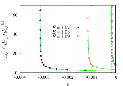
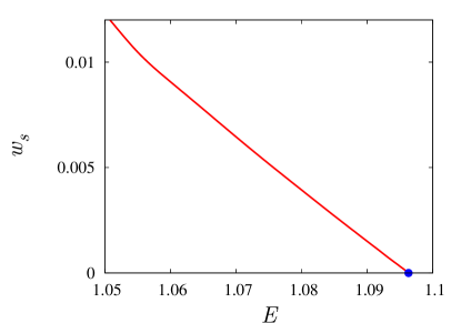
(a)                                                                      (b)

Figure 15: (a) The integrand in Eq. (82) plotted as function of $\epsilon$ for several values of total energy $E<E_{c}(E_{y})$ and $E_{y}=0.05$. The limiting values $\epsilon=\epsilon_{i}$ are shown by the vertical dotted lines. (b) The saddle point $w_{s}(E)$ at $E_{y}=0.05$.

The result for the saddle point $w=w_{s}(E)$ is plotted in Fig. 15b. As expected, $w_{s}$ is positive, decreases with energy and reaches $w_{s}=0$ at $E=E_{c}(E_{y})\approx 1.096$.

The second derivative of the suppression exponent entering Eq. (28a) is computed using the formula

$$F^{\prime\prime}(w_{s})=\frac{2\pi\hbar}{A_{pot}^{2}}\;,$$ (83)

which follows from the definition of $w$, Eq. (24). Using $w_{s}$ and $F^{\prime\prime}(w_{s})$, one finds the argument $\varkappa_{pot}$ of the Fresnel integral and thus ${\cal M}_{pot}$, see Eq. (28a).

Consider now ${\cal M}_{sph}$. From Eqs. (24), (21) one derives in a straightforward way the following expressions for the derivatives of the suppression exponent at $w=0$,

$$F^{\prime}(0)=\frac{\hbar}{A_{sph}}\;,\qquad\qquad F^{\prime\prime}(0)=\frac{1}{2}\frac{d}{dF_{\epsilon}}\left[\frac{\hbar}{A_{sph,\epsilon}}\right]_{\epsilon=0}^{2}\;.$$ (84)

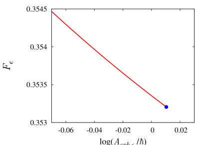
Figure 16: Suppression exponent $F_{\epsilon}$ as function of $\log A_{sph,\,\epsilon}$. The graph is plotted at $E=1.12>E_{c}(E_{y})$, $E_{y}=0.05$.

Here we denote by $A_{sph,\,\epsilon}$ the value of the r.h.s. of Eq. (22b) at finite $\epsilon$. Combining the multipliers (84), one obtains for the variable entering Eq. (28b),

$$\varkappa^{2}_{sph}=\left.-\frac{1}{2\hbar}\cdot\frac{dF_{\epsilon}}{d\log A_{sph,\,\epsilon}}\right|_{\epsilon=0}\;.$$ (85)

Note that $\varkappa_{sph}$ is real and positive. One finds it by plotting $F_{\epsilon}$ as a function of $\log A_{sph,\,\epsilon}$ at small $\epsilon$ (Fig. 16) and fitting the graph with the linear function.

Appendix F Semiclassical probability at small $E_{y}$

We showed in Sec. 6 that the probability of tunneling from the ground state of $y$-oscillator is given (up to the overall factor $(\pi/\mathrm{e})^{1/2}$) by the standard semiclassical expression, where one should use $E_{y}=\hbar\omega/2$. Let us determine explicitly the $\hbar$–dependence of this expression, i.e. extract the leading exponent and prefactor of the probability.

First, we rewrite $F_{pot}$ using the parameters $T$ and $\theta$. Namely, we evaluate the in-state term $B_{i}$ by taking the integral in Eq. (50),

$$2\mathrm{Im}\,B_{i}[\boldsymbol{x}] =\mathrm{Im}\,(y_{i}\dot{y}_{i}+x_{i}\dot{x}_{i})+\mathrm{Im}\,\left(x_{i}\dot{x}_{i}+\left(2E_{y}/\omega\right)\mathrm{arccos}(\omega y_{i}/\sqrt{2E_{y}})\right)$$

$$=\mathrm{Im}(y_{i}\dot{y}_{i}+x_{i}\dot{x}_{i})-2ET-E_{y}\theta/\omega\;,$$

where in the last equality the asymptotic form (45), (46) of the trajectory was used. For the suppression exponent (9) one obtains,

$$F_{pot}=2\mathrm{Im}\tilde{S}[\boldsymbol{x}]-2ET-E_{y}\theta/\omega\;,$$ (86)

where

$$\tilde{S}[\boldsymbol{x}]=\int dt\left[-\boldsymbol{x}\ddot{\boldsymbol{x}}/2-V(\boldsymbol{x})\right]\;$$ (87)

is the classical action integrated by parts.

The second observation is as follows. Consider the differential of the action (87) with respect to the in-state quantum numbers $E$, $E_{y}$. One writes,

$$d2\mathrm{Im}\,\tilde{S} =d\mathrm{Im}\,(2S+x_{i}\dot{x}_{i}+y_{i}\dot{y}_{i})=\mathrm{Im}\,(x_{i}d\dot{x}_{i}-\dot{x}_{i}dx_{i}+y_{i}d\dot{y}_{i}-\dot{y}_{i}dy_{i})$$

$$=2EdT+E_{y}d\theta/\omega\;.$$

This equation together with Eq. (86) show that the parameters $(T,\,\theta)$ are related to $(E,\,E_{y})$ by the Legendre transformation. Consequently,

$$dF_{pot}=-2TdE-\theta dE_{y}/\omega\;.$$

Thus, $(-2T)$ and $(-\theta/\omega)$ are equal to the derivatives of the suppression exponent with respect to $E$ and $E_{y}$.

Using the above observation, we expand the suppression exponent around the point $E_{y}=0$,

$$F_{pot}=F_{pot}\Big{|}_{E_{y}=0}-\frac{1}{\omega}\int_{0}^{E_{y}}\theta(E_{y}^{\prime})\,dE_{y}^{\prime}\;.$$

The function $\theta(E_{y})$ at small $E_{y}$ is determined by noting that

$$E_{y}=2\omega^{2}|\bar{a}|^{2}\mathrm{e}^{-2\omega T-\theta}\;,\qquad\Rightarrow\qquad\theta=-\mathrm{ln}(2E_{y}/\omega)+\theta_{0}+O(E_{y})\;,$$ (88)

where we used the fact that $|\bar{a}|$ has a well–defined limit as $E_{y}\to 0$. This yields the expression (48) for the suppression exponent. Finally, substituting Eq. (48) into Eq. (1) and recalling the additional factor $(\pi/\mathrm{e})^{1/2}$ one arrives at the expressions (47).

References

- [1] S. C. Creagh, in Tunneling in complex systems, ed. by S. Tomsovic (World Scientific, Singapore, 1998).
- [2] S. Tomsovic, Physica Scripta T90, 162 (2001).
- [3] W. H. Miller, J. Chem. Phys. 48, 1651 (1968); E. L. Sibert III, J. T. Hynes and W. P. Reinhardt, ibid. 77, 3595 (1982).
- [4] R. E. Meyer, SIAM J. Appl. Math. 51, 1585 (1991); ibid. 51, 1602 (1991).
- [5] S. C. Creagh, J. Phys. A 27, 4969 (1994).
- [6] M. Wilkinson, Physica D 21, 341 (1986); J. Phys. A 20, 635 (1987).
- [7] S. Takada and H. Nakamura, J. Chem. Phys. 100, 98 (1994); S. Takada, P. N. Walker and M. Wilkinson, Phys. Rev. A 52, 3546 (1995); S. Takada, J. Chem. Phys. 104, 3742 (1996).
- [8] S. C. Creagh and M. D. Finn, J. Phys. A 34, 3791 (2001).
- [9] G. C. Smith and S. C. Creagh, J. Phys. A 39, 8283 (2006).
- [10] O. Bohigas, S. Tomsovic and D. Ullmo, Phys. Rept. 223, 43 (1993).
- [11] E. Doron and S. D. Frischat, Phys. Rev. Lett. 75, 3661 (1995); S. D. Frischat and E. Doron, Phys. Rev. E 57, 1421 (1998).
- [12] A. Shudo and K. S. Ikeda, Phys. Rev. Lett. 74, 682 (1995); ibid. 76, 4151 (1996); Physica D 115, 234 (1998).
- [13] S. C. Creagh and N. D. Whelan, Phys. Rev. Lett. 77, 4975 (1996); ibid. 82, 5237 (1999).
- [14] A. Mouchet, C. Miniatura, R. Kaiser, B. Grémaud and D. Delande, Phys. Rev. E 64, 016221 (2001).
- [15] A. D. Ribeiro, M. A. M. de Aguiar and M. Baranger, Phys. Rev. E 69, 066204 (2004).
- [16] D. G. Levkov, A. G. Panin and S. M. Sibiryakov, Phys. Rev. E 76 046209 (2007).
- [17] A. Bäcker, R. Ketzmerick, S. Löck and L. Schilling, Phys. Rev. Lett. 100, 104101 (2008).
- [18] C. Dembowski et al, Phys. Rev. Lett. 84, 867 (2000); R. Hofferbert et al, Phys. Rev. E 71, 046201 (2005).
- [19] W. K. Hensinger et al, Nature 412, 52 (2001); W. K. Hensinger et al, Phys. Rev. A 70, 013408 (2004).
- [20] D. A. Steck, W. H. Oskay and M. G. Raizen, Science 293, 274 (2001); Phys. Rev. Lett. 88, 120406 (2002).
- [21] A. Bäcker et al, Phys. Rev. Lett. 100, 174103 (2008).
- [22] W. H. Miller, Adv. Chem. Phys. 25, 69 (1974).
- [23] M. J. Davis and E. J. Heller, J. Chem. Phys. 75, 246 (1981); E. J. Heller and M. J. Davis, J. Phys. Chem. 85, 307 (1981).
- [24] T. Onishi, A. Shudo, K. S. Ikeda and K. Takahashi, Phys Rev. E 64, 025201 (2001); ibid 68, 056211 (2003).
- [25] K. Takahashi and K.S. Ikeda, J. Phys. A 36, 7953 (2003); Europhys. Lett. 71, 193 (2005); erratum-ibid 75, 355 (2006).
- [26] F. Bezrukov and D. Levkov, arXiv:quant-ph/0301022; J. Exp. Theor. Phys. 98, 820 (2004) [Zh. Eksp. Teor. Fiz. 125, 938 (2004)].
- [27] D. G. Levkov, A. G. Panin and S. M. Sibiryakov, Phys. Rev. A 76, 032114 (2007).
- [28] D. G. Levkov, A. G. Panin and S. M. Sibiryakov, Phys. Rev. Lett. 99, 170407 (2007).
- [29] K. Takahashi and K. S. Ikeda, Phys. Rev. Lett. 97, 240403 (2006).
- [30] K. Takahashi and K. S. Ikeda, J. Phys. A 41, 095101 (2008).
- [31] A. Shudo, Y. Ishii and K. S. Ikeda, Europhys. Lett. 81, 50003 (2008).
- [32] F. Bezrukov, D. Levkov, C. Rebbi, V. Rubakov and P. Tinyakov, Phys. Rev. D 68, 036005 (2003); Phys. Lett. B 574, 75 (2003).
- [33] D. G. Levkov and S. M. Sibiryakov, Phys. Rev. D 71, 025001 (2005); JETP Lett. 81, 53 (2005) [Pisma Zh. Eksp. Teor. Fiz. 81, 60 (2005)].
- [34] F. R. Klinkhamer and N. S. Manton, Phys. Rev. D 30, 2212 (1984).
- [35] S. Wiggins, L. Wiesenfeld, C. Jaffé and T. Uzer, Phys. Rev. Lett. 86, 5478 (2001).
- [36] V. A. Rubakov, D. T. Son and P. G. Tinyakov, Phys. Lett. B 287, 342 (1992).
-
[37]
M. P. Mattis, Phys. Rept. 214, 159 (1992);
P. G. Tinyakov, Int. J. Mod. Phys. A 8, 1823 (1993);
V. A. Rubakov and M. E. Shaposhnikov, Phys. Usp. 39, 461 (1996) [Usp. Fiz. Nauk 166, 493 (1996)]. - [38] G. F. Bonini, A. G. Cohen, C. Rebbi and V. A. Rubakov, Phys. Rev. D 60, 076004 (1999); quant-ph/9901062.
- [39] http://solver.inr.ac.ru
- [40] I. Affleck, Nucl. Phys. B 191, 429 (1981).
- [41] D. G. Levkov, A. G. Panin, to be published.
- [42] M. V. Berry, K. E. Mount, Rept. Prog. Phys. 35, 315 (1972).
- [43] J.H. Van Vleck, Proc. Natl. Acad. Sci. USA 14, 178 (1928).
- [44] H. Kleinert, Path Integrals in Quantum Mechanics, Statistics, Polymer Physics, and Financial Markets, World Scientific, Singapore, 2006.
- [45] A. N. Kuznetsov and P. G. Tinyakov, Phys. Rev. D 56, 1156 (1997).
- [46] W. H. Press et al, Numerical recipes in C: the art of scientific computing, Cambridge University Press, 1992.