Unveiling the high energy tail of 1E 1740.7–2942 with INTEGRAL

Abstract

The microquasar 1E 1740.7–2942  is observed with INTEGRAL since Spring 2003. Here, we report on the source high energy behaviour by using the first three years of data collected with SPI and IBIS telescopes, taking advantage of the instruments complementarity. Light curves analysis showed two main states for 1E 1740.7–2942: the canonical low/hard state of black-hole candidates and a “dim” state, characterised by a $\sim$ 20 times fainter emission, detected only below 50 keV and when summing more than 1Ms of data. For the first time the continuum of the low/hard state has been measured up to $\sim 600$ keV with a spectrum that is well represented by a thermal Comptonization plus an additional component necessary to fit the data above 200 keV. This high energy component could be related to non-thermal processes as already observed in other black-hole candidates. Alternatively, we show that a model composed by two thermal Comptonizations provides an equally representative description of the data: the temperature of the first population of electrons results as (kT_e)${}_{1}\sim$ 30 keV while the second, (kT_e)₂, is fixed at 100 keV.

Finally, searching for 511 keV line showed no feature, either narrow or broad, transient or persistent.

1 Introduction

1E 1740.7–2942 is a bright hard X-ray source located at less than one degree off the Galactic Centre (Hertz & Grindlay 1984; Cook et al. 1991; Roques et al. 1991), classified as Black Hole Candidate (BHC; e.g. Sunyaev et al. 1991). When Mirabel et al. (1992) discovered a double sided radio jet reaching large angular distances from the core ($\sim$ 1’), the ”microquasar” class was born with 1E 1740.7–2942 as its first member.
All observations performed so far revealed that 1E 1740.7–2942 spends most of the time in the canonical Low/Hard (LH) state of BHCs (Smith et al. 2002 and ref. therein). In this state, the X/$\gamma$ ray spectrum is empirically described by a power-law with a photon index of 1.4-1.5 plus a roll-over around 100 keV Zdziarski (2000). In a few occasions, soft spectral states have been observed during 1E 1740.7–2942 low flux levels Smith et al. (2002). Moreover, simultaneous INTEGRAL and RXTE broad-band spectral study performed in 2003 report on an intermediate/soft spectral state occurred just before the source quenching Del Santo et al. (2005).

In 1990, the SIGMA telescope on-board GRANAT detected a broad line around the electron-positron annihilation energy (Bouchet et al. 1991; Sunyaev et al. 1991). This transient feature appeared clearly during a 13 hours observation and then possibly in two further occasions but at a less significant level. Numerous works dedicated to similar line searches have followed and all led to negative conclusions (see for example Cheng et al. 1998 and references therein). In this context, it is interesting to perform a deep analysis of SPI data in this energy domain, and to seek for any feature around 511 keV associated with 1E 1740.7–2942.
The superior energy resolution of the SPI telescope allows for a specific dedicated study of this topic. Indeed, for the first time, an instrument is capable to look for a narrow feature in this particular source. During the first year of observations, no evidence for point source emission at 511 keV has been detected with SPI. The upper limit at 3.5 $\sigma$ level is $1.6\times 10^{-4}$ ph cm^-2 s^-1 for a narrow line (Teegarden & Watanabe 2006) while the IBIS data set a 2 $\sigma$ upper limit of $1.6\times 10^{-4}$ ph cm^-2 s^-1 in the 535-585 keV energy band for an exposure time equal to 1.5 Ms (De Cesare et al. 2006).

We report here on the high-energy spectral properties as revealed with the INTEGRAL high-energy instruments. The sensitivity and imaging capabilities of IBIS/ISGRI allow to determine the contribution of all the emitting sources in large fields of view, while the SPI telescope brings some additional spectral informations above 150-200 keV with a deep investigation of the 511 keV line status.

2 INTEGRAL Observations

Since its launch on October 17th 2002, INTEGRAL Winkler et al. (2003) observed the Galactic Center region two times per year, in the Spring and Fall visibility windows. Observations are performed in dither pattern with each pointing (named science window, SCW) lasting beetwen 1700 and 3600 seconds. We have analysed all public data collected between Spring 2003 and Fall 2005 by the spectrometer SPI Vedrenne et al. (2003) and the imager IBIS Ubertini et al. (2003).

After image analysis and cleaning, the useful data set consists in about 3500 exposures for a total useful time of 8 Ms divided in 6 periods (Spring and Fall, 2003, 2004 and 2005, see Table 1).

3 Data analysis

3.1 IBIS

The unprecedented IBIS Ubertini et al. (2003) angular resolution combined with sensitivity ($<$1 mCrab for 1 Ms ; Bird et al. 2007) allow us to resolve sources lying in crowded field, as the Galactic Centre. The IBIS Partially Coded Field Of View is 29${}^{\circ}\times$29^∘ at zero response, but the full instrument sensitivity is achieved in the 9${}^{\circ}\times$9^∘ Fully Coded Field of View. For our aims, we selected IBIS observations including 1E 1740.7–2942  in the FOV up to 50% coding (19${}^{\circ}\times$19^∘; see Tab. 1). In this paper, we refer to data collected with the IBIS low energy detector, ISGRI Lebrun et al. (2003), covering the 15-1000 keV energy band.

The IBIS scientific analysis has been performed using the INTEGRAL off-line analysis software, OSA Goldwurm et al. (2003). The IBIS/ISGRI images have been extracted SCW by SCW in three energy bands, i.e. 20-40 keV, 40-100 keV and 100-300 keV. Mosaic images by revolution have been used to measure fluxes of all sources within 2 degree off 1E 1740.7–2942 used as input for SPI analysis (see Section 3.2.1).
Spectra have been extracted SCW by SCW in 35 logarithmic bins spanning from 20 keV to 600 keV. The response matrices (RMF and ARF) used for spectral fitting are those delivered with OSA 5.1 distribution. To take into account the improvements included in the matrices delivered in OSA-7, we modified the ISGRI spectra by the factors corresponding to ratios between the Crab spectra measured respectively with OSA-5 and OSA-7 packages.

3.2 SPI

In addition to its spectroscopic capability, SPI can image the sky with a spatial resolution of $2.6^{\circ}$ (FWHM ) over a field of view of $30^{\circ}$ (Roques et al. 2003).
The signal recorded by SPI camera consists of the contributions from sources in the field of view plus background. A system of equations is to be solved to determine sources and background intensities. In order to reduce the number of unknowns necessary to describe the data, we introduce some known information on both components. For the background, the relative count rates of the 19 Ge detectors (uniformity maps) are very stable and can be kept constant within each considered period (see Table 1) while the global normalisation factor is determined by 6 hours intervals. Concerning the sources, timescales are chosen in function of the source intensity and temporal behaviour, the faintest ones being considered as constant. Detailed description of the data analysis algorithms and methods, using matrices available in the OSA package, can be found in Bouchet et al. (2005; 2008).
Exposures were selected on the basis of their pointing direction which is here required to be less than $12^{\circ}$ from 1E 1740.7–2942. This ensures to keep the maximum sensitivity for 1E 1740.7–2942 and reduces the total field of view spanned by the observations, leading to a simpler description of the sky.

3.2.1 SPI correction from IBIS inputs

The region around 1E 1740.7–2942 is particularly crowded (Bird et al. 2007; Belanger et al. 2006). Due to the modest SPI angular resolution ($\sim 2.6^{\circ}$), the spectrum directly extracted at 1E 1740.7–2942 position may contain contributions from other weak/close/“not seen” sources. Nevertheless, it is possible to obtain the emission spectrum of 1E 1740.7–2942 from SPI data thanks to the information provided by IBIS/ISGRI.

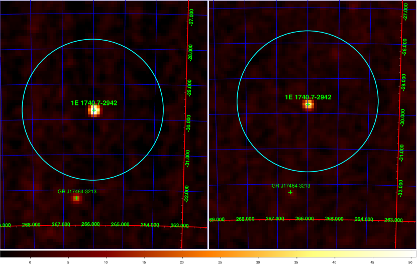
Figure 1: IBIS images of the 1E region in 2003 (left) and 2005 (right) in the 100-300 keV energy range. The cyan circles are $2^{\circ}$ in radius.

For that, we need to determine the fraction of the flux extracted at the 1E 1740.7–2942 position that actually originates from the source itself. This has been determined by a set of simulations. The first step consists to extract the flux of all emitting sources in its neighbourhood measured by IBIS. We then simulate the counts projected by them on the SPI detector plane, taking into account the complete (angular dependent) SPI response. Applying the standard analysis method to these simulated data gives us a ”1E 1740.7–2942 region” flux, that we can compare to the 1E 1740.7–2942 flux injected as input in the simulation. The ratio between these two fluxes corresponds to the factor we have to apply to correct the flux measured by SPI at the 1E 1740.7–2942 position in the observed data to obtain the flux attributable to the source itself. This procedure has been repeated in a few broad bands and for each observational period. This cleaning procedure takes into account a global contribution of all potential contaminations, and the corresponding IBIS error bars can be considered as very small compared to the SPI ones. However, the contamination effect which is important in the low-energy domain, becomes negligible when going up to higher energies. In fact, as can be seen in Fig. 1, above 100 keV only 1E 1740.7–2942 is detected with a significant flux within $2^{\circ}$ off the source.

3.2.2 Modelling the diffuse background : e+e- annihilation line and positronium emission

The SPI design makes it sensitive to both source and diffuse emissions. On the other hand, the Galactic Centre (GC) region is dominated in the $\sim$ 300 keV up to 511 keV domain by the Galactic diffuse annihilation radiation. The annihilation line emission is detected with SPI with a flux of $\sim 1\times 10^{-3}$ ph cm^-2 s^-1 and a $\sim 8^{\circ}$ axisymmetric Gaussian spatial distribution centered at the Galactic Centre Knödlseder et al. (2005); Bouchet et al. (2008). 1E 1740.7–2942 continuum emission around 511 keV is expected to be (in the “hard state”) of the order of a few percents of the galactic background line intensity. It is thus crucial for our work to determine this latter accurately. This task has been performed using a larger data set (see Bouchet et al. 2008), which includes observations at larger latitudes and longitudes.

The diffuse emission has been described in this process by two gaussians while eight known sources has been introduced as potential emitters (including 1E 1740.7–2942). Thus, the fitting algorithm (based on a $\chi^{2}$ minimization method, see Bouchet et al. 2008 for more details) is able to adjust simultaneously point sources fluxes and the diffuse component contribution in the 511 keV line domain. The energy centroid and width of the positron annihilation line were fixed at 511 keV and 2.5 keV FWHM respectively Churazov et al. (2005). The fit procedure results in a model consisting in two Gaussians with FWHM of 3.2^∘ and 10.8^∘ and fluxes of 2.3 and 7.0 $\times 10^{-4}$ ph cm^-2 s^-1  respectively, as the best description of the annihilation line spatial distribution and flux, without any significant emission from the point sources (see Weidenspointner et al. 2008, supplementary material, for independent analysis).
Concerning the positronium we assumed it to follow the same two Gaussians spatial distribution as the 511 keV line and determined its flux by the same fitting procedure. This results in a positronium fraction of 0.98, a value that is compatible with all SPI measurements Bouchet et al. (2008).
Finally, the contributions of these Galactic diffuse components on the detector plane are subtracted from the data in the counts space.

4 Results

4.1 Temporal analysis

Table 2 gives the 1E 1740.7–2942 averaged fluxes for the different periods in two broad bands. The source mean hardnesses in 2003 and 2005 are similar indicating that 1E 1740.7–2942 was in the LH state. Its intensity is rather stable on the revolution timescale, within 40 and 60 mCrab in the 20-40 keV energy band, except in the fall 2003 period, during which a continous decrease, from 85 to 27 mCrab, preceded the quenching observed in 2004 Del Santo et al. (2005). Indeed, in 2004, the source was weaker with no detection above 5 $\sigma$ within individual revolutions. The data accumulation by periods allows to determine a mean flux of a few mCrab.

A dedicated study in a narrow (10 keV) band around 511 keV has been used to search for any transient emission from the annihilation process. We have tested 0.5 day and 1 day timescales without detecting any significant emission. The actual durations of each temporal bin depends on the observational planning and is thus variable. The 2 $\sigma$ upper limits range from $4.2\times 10^{-4}$ ph cm^-2 s^-1 to $3.6\times 10^{-3}$ ph cm^-2 s^-1 with an averaged value $\sim 8\times 10^{-4}$ ph cm^-2 s^-1  for a 0.5 day timescale, and from $3.1\times 10^{-4}$ ph cm^-2 s^-1 to $2.3\times 10^{-3}$ ph cm^-2 s^-1 with an averaged value of $6.8\times 10^{-4}$ ph cm^-2 s^-1  for a day timescale. These results are illustrated by the distribution of the measurements in $\sigma$ unit for the 12 hours timescale (Fig 2, solid line) while a 2 $\sigma$ upper limit of $4.8\times 10^{-5}$ ph cm^-2 s^-1 is deduced for the total duration (see Table 2 for upper limits by periods).
Finally, a study has been performed for a broad feature, based on the 240 keV width (FWHM) reported in SIGMA data (Bouchet et al. 1991, Sunyaev et al. 1991). The continuum emission (not negligible in such a broad band) has been estimated by the mean flux over the considered period and subtracted from the data. Here too, no significant excess above the expected continuum emission can be claimed over the 2003-2005 periods (Fig. 2, dashed line). The 2 $\sigma$ upper limits span from $1.7\times 10^{-3}$ ph cm^-2 s^-1 to $1.3\times 10^{-2}$ ph cm^-2 s^-1 with an averaged value close to $3\times 10^{-3}$ ph cm^-2 s^-1, for a 0.5 day timescale, and from $1.2\times 10^{-3}$ ph cm^-2 s^-1 to $8.8\times 10^{-3}$ ph cm^-2 s^-1 with an averaged value of $2.5\times 10^{-3}$ ph cm^-2 s^-1, for a day timescale. Note that the line flux reported by SIGMA was $1.3\times 10^{-2}$ ph cm^-2 s^-1.

4.2 Spectral analysis

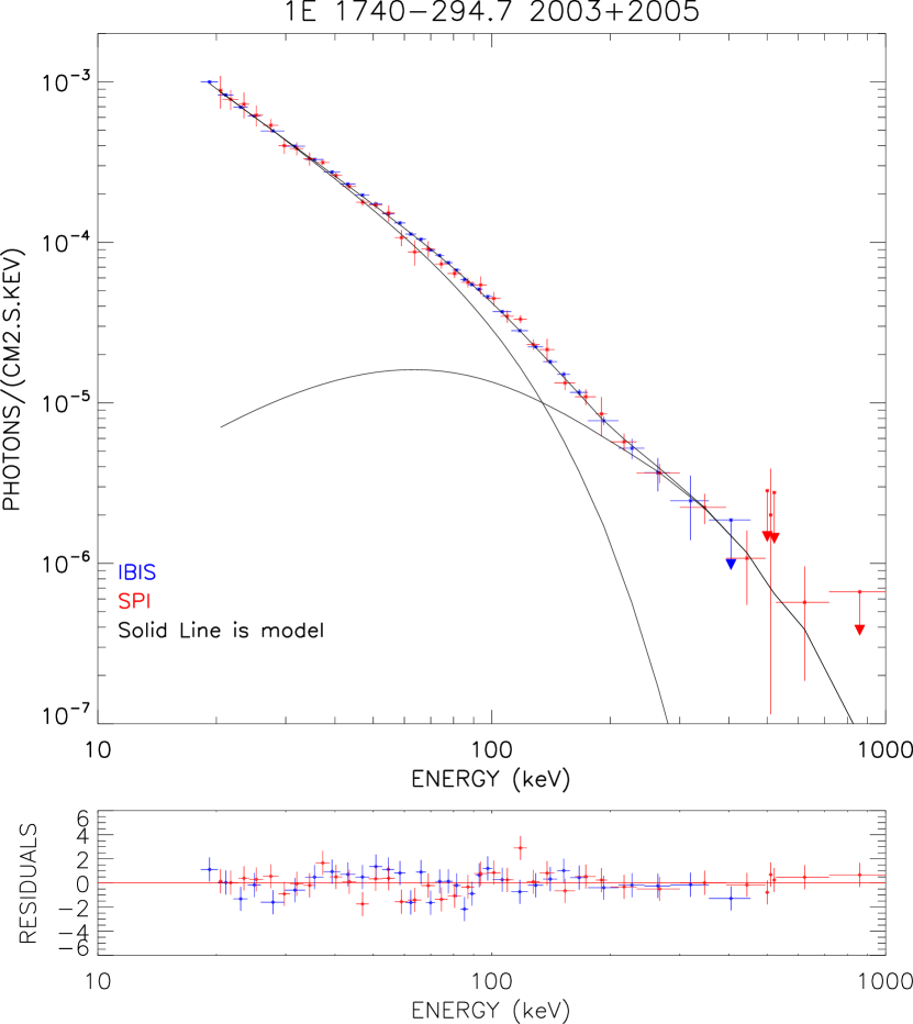
Figure 3: 1E 1740.7–2942 spectrum observed by IBIS and SPI for 2003 + 2005 observations. Solid line is a two comptonisation model (2* comptt), with hotter temperature fixed to 100 keV. The other parameters are described in the text.

After correction of the SPI data (Section 3.2.1), SPI and IBIS/ISGRI spectra have been fitted simultaneously. We have first built averaged spectra for 2003 and 2005 separately. In a second step, being the source in a similar state during these two periods, we achieved an averaged LH state spectrum in order to obtain a better statistics at high energy.
Spectral fitting of these 3 data sets have been performed with the standard XSPEC v.11.3.1 tools. We have included a normalisation factor during each fitting procedure and noticed that it remains between 0.94 and 1.0 (ISGRI factor fixed to 1.0). Indeed, SPI spectra are very similar to the ISGRI ones (as illustrated in fig. 3), even if they present some fluctuations at low energy, easily understandable in terms of residual cross-talk between neighbouring sources. However, this effect is limited and even negligible above $\sim$ 100 keV.
During both periods, the source emission extends up to 500 keV with a spectral shape presenting a clear cutoff around $\sim$ 140 keV. This cutoff is undoubtedly required by the $\chi^{2}$ statistics: we obtain $\chi_{\nu}^{2}$ of 10 and 6.6 (for 71 dof) with a power-law model, while adding a high-energy cutoff these values result as 0.9 and 1.14 (70 dof).
Then we used a Comptonization model (comptt, Titarchuk 1994) as this mechanism is expected to play the major role in our energy domain and to produce such a cutoff. We obtain electron temperatures (kT_e) of roughly 50 keV with optical depthes ($\tau$) close to 1 (see Tab. 3), that are quite canonical values for this class of objects. However, the 2005 and total (2003+2005) spectra give high $\chi_{\nu}^{2}$ values (1.35 and 1.8 for 69 dof). These, combined with residuals at high energy, suggest the presence of a supplementary component explaining data points above 200 keV. We have studied this hypothesis in the total spectrum since its statistics allows us to better constrain the spectral parameters. In order to model the high-energy data, we added a power law component and obtain a $\chi_{\nu}^{2}$ close to 1 with a photon index of 1.9 $\pm$ 0.1. The plasma temperature is thus decreased as 27 $\pm$ 2.2 keV with $\tau$ = 1.9 $\pm$ 0.25.
Even though this two components model is quite satisfying, with a classical explanation of a non-thermal process responsible of the power-law emission, as in High Soft States, we also made an attempt to test whether alternative scenario with only thermal mecanisms were excluded.
Indeed, a two (thermal) Comptonization model gives a similarly acceptable description of the spectrum. The constraints on the parameters are very poor, so we impose a second population temperature at 100 keV and consider that it comptonizes photons coming from the first Comptonizing region, i. e. (kT_seed)₂ = (kT_e)${}_{1}\sim$ 30 keV. The optical depthes of both regions are found similar and compatible (1.6 $\pm$ 0.1 and 2.2 $\pm$ 0.8) while the $\chi_{\nu}^{2}$ = 1.07 (67 dof) leads to an F-test probability of $\sim 10^{-8}$ for the existence of such a second component. Results corresponding to this scenario are displayed in Fig. 3 and Tab. 3. Since this analysis is strongly based on ISGRI data at low energy, we performed a fit using SPI data above 100 keV only (no contamination effect) and found that the parameters are unchanged.

5 Discussion and conclusions

Even though the 1E 1740.7–2942  region is particularly difficult to analyse with the SPI telescope, we have demonstrated that the use of the IBIS and SPI complementarity allows us to get a common spectrum of 1E 1740.7–2942  itself. Thanks to the inputs from the ISGRI detector, we have estimated the relative contribution of all sources active in a $1^{\circ}$ circle around 1E 1740.7–2942  and showed that we can reconstruct the SPI 1E 1740.7–2942  spectrum with a precision better than 5 % relatively to the ISGRI one.

Two main states have been observed: the canonical LH state with a flux of $\sim$ 50 mCrab and 60 mCrab in the 20-40 keV and 40-100 keV bands respectively, and a ”dim” state during which the flux of 1E 1740.7–2942 is below the IBIS/ISGRI detection limit on the revolution timescale and detected at a level of 2.6 -2.7 mCrab (14 $\sigma$) when integrated over $\sim$ 3 months periods.
Spectra have been built for periods when the source was clearly detected (2003, 2005 and the sum of both). The problematic of the SPI analysis leads to rather large error bars but in all cases, the emission extends up to $\sim$ 500 keV, even though a high energy cutoff appears clearly in the data. When adjusted with a single Comptonization model, an additional component is strongly required to fit the data above 200 keV, particularly in the total spectrum because of the very significant emission at these energies.
This high energy component has been observed in several BHCs (e.g. McConnell et al. 2000; Zdziarski et al. 2001), usually during high soft spectral states, and explained as Compton up-scattering by a non-thermal electrons population Zdziarski & Gierliński (2004). As alternative scenario, jets can easily produce hard X-ray emission via synchrotron radiation in addition to the inverse Compton scattering Markoff et al. (2003). However, by computing radio-to-gamma ray Spectral Energy Distribution, Bosch-Ramon et al. (2006) ruled out the jet emission for the hard-X ray spectrum of 1E 1740.7–2942, favoring rather the corona origin.
Recently, high energy excesses have been observed in transient BHCs when in LH state (i. e. Del Santo et al. 2008; Joinet et al. 2007), that could be the result of spatial/temporal variations in plasma parameters Malzac & Jourdain (2000). We have demonstrated with our data that, for the LH state spectrum of 1E 1740.7–2942, a model consisting of two thermal Comptonization components, with a second hotter population ((kT_e)₂ fixed to 100 keV) interacting with the photons produced by the first one, provides an interesting alternative to the non-thermal scenarios. This two temperature model could either correspond to two distinct heating mecanisms/regions or reflect the presence of a gradient of temperature in the Comptonising plasma.

Finally, even though the complexity of the considered region makes it difficult to attribute firmly the detected emission to 1E 1740.7–2942, the presence of photons with energy greater than several hundreds of keV in a more or less persistent way (something as half or 2/3 of the time), together with previously reported annihilation emission, support a scenario in which 1E 1740.7–2942 is a source of positrons. Indeed, as proposed by van Oss & Belyanin (1995), a plasma detected with a temperature much lower than 1 MeV is able to produce positrons throught photon-photon absorption. The basic argument is that the hard X-ray emission comes from the regions close to the central black hole, where the gravity field is very strong. The high local temperature is thus lowered, leading to an observed value far from the relativistic domain, while pairs are created in the innermost disk and driven away. Annihilation outbursts could occur when the accretion flow intercepts the pair wind (van Oss & Belyanin 1995).
Concerning the 511 keV line itself, no feature, broad or narrow, transient or persistent, has been found, confirming the rare occurence of such a phenomenon in line with numerous different studies already performed on this topics. It is worth to note, however, that SPI/INTEGRAL gives the first opportunity to investigate it in terms of narrow feature (a few keV) with actual constraints on its parameters. Unfortunately, any strong conclusion would require more information on the expected duration (and width) of the emission.

Table 1: Observations log.

Period	Start Time	End Time	Pointings (or Scw)	Exposure (Ms)
	(UT)	UT	IBIS / SPI	IBIS / SPI
2003 spring	2003 Feb 28	2003 Apr 22	298 / 434	0.62 / 0.86
2003 autumn	2003 Aug 19	2003 Oct 9	717 / 709	2.26 / 2.14
2004 spring	2004 Feb 17	2004 Apr 20	547 / 544	1.29 / 1.18
2004 autumn	2004 Aug 21	2004 Oct 28	747 / 610	1.78 / 1.35
2005 spring	2005 Feb 16	2005 Apr 20	802 / 697	1.48 / 1.27
2005 autumn	2005 Aug 16	2005 Oct 5	353 / 407	0.70 / 0.93

Table 2: Averaged 1E 1740.7–2942 flux by periods. For the 511 keV feature, 2$\sigma$ upper limits are given for a narrow line ($\Delta$ E = 10 keV).

Period	2003 spring	2003 fall	2004 spring	2004 fall	2005 spring	2005 fall	2003 & 2005	2004	total period
$F_{20-40keV}$	51	75	2.6	2.7	53	53	62
mCrab
$F_{40-100keV}$	60	95	-	-	56	54	68
mCrab
$F_{511keV}\times 10^{-4}$	$<$ 1.22	$<$ 0.66	$<$ 1.02	$<$ 1.10	$<$ 1.10	$<$ 1.32	$<$ 0.48	$<$ 0.74	$<$ 0.40
ph cm-2 s-1

Table 3: The best fit parameters for the combined ISGRI and SPI 1E 1740.7–2942 spectra with Comptonization model (comptt, Titarchuk 1994). T0 is fixed to 0.3 keV. For the 2003+2005 spectrum, the second line corresponds to a 2 Comptonization model ((kT_e)₁ , $\tau_{1}$, (kT_e)₂ , $\tau_{2}$) with the 2nd seed photon temperature fixed to (kT_e)₁ and (kT_e)₂ fixed to 100 keV (see text).

period	(kTe)1	$\tau_{1}$	(kTe)2	$\tau_{2}$	$\chi_{\nu}^{2}$ (dof)	F-test (1)
	keV		keV
2003	50.1 $\pm$ 2.6	1.00 $\pm$ 0.06			1.1 (69)
2005	45.4 $\pm$ 2.7	1.10 $\pm$ 0.08			1.35 (69)
2003+2005	48.1 $\pm$ 2.0	1.06 $\pm$ 0.05			1.8 (69)
2003+2005	29.4 $\pm$ 3.1	1.6 $\pm$0.1	100	2.2 $\pm$ 0.8	1.07 (67)	10-8

Figure 2: Distributions of the fluxes measured for the 511 keV line in sigma units, for two hypotheses (a narrow feature: solid line, a broad feature: dashed line).

References

- Belanger et al. (2006) Belanger. G., Goldwurm, A., Renaud, M., et al. 2006, ApJ, 636, 275
- Bird et al. (2007) Bird, A.J., Malizia, A., Bazzano, A., et al. 2007, ApJS, 170, 175
- Bosch-Ramon et al. (2006) Bosch-Ramon, V., Romero, G. E., Paredes, J. M., Bazzano, A., Del Santo, M. & Bassani, L. 2006, A&A, 457, 1011
- Bouchet et al. (1991) Bouchet, L. et al. 1991, ApJ, 383, L45
- Bouchet et al. (2005) Bouchet, L., Roques, J. P., Mandrou, P., Strong, A., Diehl, R., Lebrun, F. & Terrier, R. 2005, ApJ, 635, 1115
- Bouchet et al. (2008) Bouchet, L., Jourdain, E., Roques, J. P., Strong, A., Diehl, R., Lebrun, F. & Terrier, R. 2008, ApJ, 679, 1315
- Cheng et al. (1998) Cheng, L. X., Leventhal, M., Smith, D., Gehrels, N., Tueller, J. and Fishman, G., 1998, ApJ, 503, 809
- Churazov et al. (2005) Churazov, E., Sunyaev, R., Sazonov, S., Revnivtsev, M. & Varshalovich, D. 2005, MNRAS, 357, 1377
- Cook et al. (1991) Cook, W.R., Grunsfeld, J. M., Heindl, W. A., Palmer, D. M., Prince, T. A., Schindler, S. M. & Stone, E. 1991, ApJL, 372, L75
- De Cesare et al. (2006) De Cesare, G., Bazzano, A., Capitanio, F., Del Santo, M., Lonjou, V., Natalucci, L., Ubertini, P. & von Ballmoos, P. 2006, AdvSpR, 38, 1457
- Del Santo et al. (2005) Del Santo, M. et al. 2005, A&A, 433, 613
- Del Santo et al. (2008) Del Santo, M., Malzac, J., Jourdain, E., Belloni, T. & Ubertini, P. 2008, MNRAS, in press. astro-ph 0807.1018
- Goldwurm et al. (2003) Goldwurm, A. et al. 2003, A&A, 411, L223
- Hertz & Grindlay (1984) Hertz, P. & Grindlay, J. E. 1984, ApJ, 278, 137
- Joinet et al. (2007) Joinet, A., Jourdain, E., Malzac, J., Roques, J. P., Corbel, S., Rodriguez, J., & Kalemci, E. 2007, ApJ, 657, 400
- Knödlseder et al. (2005) Knödlseder J. et al. 2005, A&A, 441, 513
- Lebrun et al. (2003) Lebrun, F. et al. 2003, A&A, 411, L141
- Malzac & Jourdain (2000) Malzac, J., & Jourdain, E. 2000, A&A, 359, 843
- Markoff et al. (2003) Markoff, S., Nowak, M., Corbel, S., Fender, R., Falcke, H. 2003, A&A, 397, 645
- McConnell et al. (2000) McConnell, M. L. et al. 2000, ApJ, 543, 928
- Mirabel et al. (1992) Mirabel, F., Rodriguez, L. F., Cordier, B., Paul, J. & Lebrun, F. 1992, Nature, 358, 215
- van Oss & Belyanin (1995) van Oss, R. F. & Belyanin, A. A., 1991, A&A., 302, 154
- Roques et al. (1991) Roques, J.P. et al. 1991, AdSpR, 11, 869
- Roques (2003) Roques J.P. et al 2003, A&A, 411, L91
- Smith et al. (2002) Smith, D. M., Heindl, W. A. & Swank, J. H. 2002, ApJ, 569, 362
- teegarden & Watanabe (2006) Teegarden, B. J. & Watanabe, 2006, ApJ, 646, 965
- Sunyaev et al. (1991) Sunyaev, R. et al. 1991, ApJ, 383, L49
- Titarchuk (1994) Titarchuk, L. 1994, ApJ, 434, 313
- Ubertini et al. (2003) Ubertini, P. et al. 2003, A&A, 411, L131
- Vedrenne et al. (2003) Vedrenne, G. et al. 2003, A&A, 411, L63
- Weidenspointner et al. (2008) Weidenspointner, G. et al. 2008, Nature, 451, 159
- Winkler et al. (2003) Winkler, C. et al. 2003, A&A, 411, L1
- Zdziarski (2000) Zdziarski, A. A. 2000, IAUS, 195, 153
- Zdziarski et al. (2001) Zdziarski, A. A., Grove, E., Poutanen, J., Rao, A. R. & Vadawale, S. V. 2001, ApJL, 554, L45
- Zdziarski & Gierliński (2004) Zdziarski, A. A., Gierliński 2004, Progress of theoretical Physics, 155, 99