Opacity effects and shock-in-jet modelling of low-level activity in Cygnus X-3

Abstract

We present simultaneous dual-frequency radio observations of Cygnus X-3 during a phase of low-level activity. We constrain the minimum variability timescale to be 20 min at 43 GHz and 30 min at 15 GHz, implying source sizes of 2–4 AU. We detect polarized emission at a level of a few per cent at 43 GHz which varies with the total intensity. The delay of $\sim 10$ min between the peaks of the flares at the two frequencies is seen to decrease with time, and we find that synchrotron self-absorption and free-free absorption by entrained thermal material play a larger role in determining the opacity than absorption in the stellar wind of the companion. A shock-in-jet model gives a good fit to the lightcurves at all frequencies, demonstrating that this mechanism, which has previously been used to explain the brighter, longer-lived giant outbursts in this source, is also applicable to these low-level flaring events. Assembling the data from outbursts spanning over two orders of magnitude in flux density shows evidence for a strong correlation between the peak brightness of an event, and the timescale and frequency at which this is attained. Brighter flares evolve on longer timescales and peak at lower frequencies. Analysis of the fitted model parameters suggests that brighter outbursts are due to shocks forming further downstream in the jet, with an increased electron normalisation and magnetic field strength both playing a role in setting the strength of the outburst.

1 Introduction

Cygnus X-3 is one of the few persistently bright radio-emitting X-ray binary systems in our Galaxy. It exhibits resolved relativistic jets during its occasional giant outbursts, which have been directly imaged on milliarcsecond scales (Mioduszewski et al., 2001; Miller-Jones et al., 2004; Tudose et al., 2007) with very long baseline interferometry (VLBI). While the giant outbursts are the most spectacular and well-studied type of radio behaviour, the system remains active at a lower level for most of the time. Waltman et al. (1994) identified three different types of variability; normal quiescent emission (60–140 mJy, variable on a timescale of months), periods of frequent small flaring ($<1$ Jy), and the major ($>10$ Jy) or intermediate ($>1$ Jy) flares, with their associated pre-flare quench periods. These classifications were based on dual-frequency data from the Green Bank Interferometer, with 10-min observations made 3–5 times per day. Waltman et al. (1996) deduced from the higher-than-expected scatter in the quiescent flux densities that irregular flux variations continue to be present in this low-level state, particularly at the higher frequencies, and data at higher time resolution has shown that the so-called “quiescent” state is in fact variable on much shorter timescales (Molnar, Reid & Grindlay 1984, 1985, 1988), of order tens of minutes. Far from being quiescent, the source is continuously active at a low level, aside from the pre-flare periods of truly quenched emission.

Newell, Garrett & Spencer (1998) observed some minor flaring episodes (peak fluxes $\sim 300$ mJy) with the Very Long Baseline Array (VLBA) and claimed evidence for superluminal expansion and contraction of the source. No other high-resolution observations have addressed the nature of the source during the low-level, active state in which it spends the majority of its time. The resolved nature of the source in the observations of Newell et al. (1998) demonstrated that the jets are still active even outside the major flaring events. Direct evidence for jet activity outside flaring events is also seen in GRS 1915+105, in which an AU-scale nuclear jet was resolved with the VLBA (Dhawan, Mirabel & Rodríguez, 2000). At the resolution of the images, the jet was observed to be continuous rather than knotty, with a length which varied with observing wavelength as $\sim 10\lambda_{\rm cm}$ AU. The lightcurves of the observations confirmed that this was an optical depth effect. We see emission from the $\tau=1$ surface, which is further out at lower frequencies. This then results in a time delay between flux variations at different frequencies, as any injection of relativistic plasma at the jet base takes time to propagate out to the point at which the jet is optically thin at the observing frequency (as seen in GRS 1915+105 by Mirabel et al., 1998). This also gives rise to the smoothing out of the variability at lower frequencies, since the observed emission is a convolution over a larger region. Measurements of the time delay between different observing frequencies can thus help constrain the size scale of the jets.

Being optically thick, such self-absorbed jets tend to show very low levels of linear polarization. Corbel et al. (2000) detected linear polarization at a level of $\sim 2$ per cent in the jets of GX 339-4 while the source was in the low/hard X-ray state (believed to be associated with steady, low-level jets). The position angle of the electric field vector remained constant over more than two years, indicating a favoured axis in the system, believed to be aligned with the axis of the compact jets. Transient jets, on the other hand, regularly show significantly higher levels of polarized emission, arising from optically thin ejecta (e.g. Fender et al., 1999; Hannikainen et al., 2000; Brocksopp et al., 2007), which may vary in amplitude and position angle with time, as different components dominate the flux density at different times, or if the source moves out from behind a screen of ionised electrons which rotate the position angle via Faraday rotation.

The relativistically-moving transient ejecta observed during X-ray binary outbursts (e.g. Mirabel & Rodríguez, 1994; Fender et al., 1999; Tingay et al., 1995; Hjellming & Rupen, 1995) have previously been modelled either as discrete knots of adiabatically-expanding plasma (e.g. van der Laan, 1966; Hjellming & Johnston, 1988; Atoyan & Aharonian, 1999), or as internal shocks within a pre-existing steady flow (e.g., Fender, Belloni & Gallo, 2004). Atoyan & Aharonian (1999) found that a discrete plasmon model requires continuous replenishment of relativistic particles as well as radiative, adiabatic, and energy-dependent escape losses. Kaiser, Sunyaev & Spruit (2000) argued that such energy-dependent escape losses were inconsistent with continuous particle replenishment via shock acceleration, and adapted the internal shock model originally derived for AGN jets (Rees, 1978; Marscher & Gear, 1985) to X-ray binary systems. Fender et al. (2004) integrated the internal shock scenario into a model explaining the disc-jet coupling over the entire duty cycle of an X-ray binary system. In this scenario, as a source moves from a hard to a soft X-ray state, the bulk Lorentz factor of the pre-existing steady jet increases, giving rise to shocks where the highly-relativistic plasma catches up with pre-existing slower-moving material downstream in the jets. In this work, we focus on the shock-in-jet model, since internal shocks form a natural explanation for the outbursts in the current disc-jet coupling picture (Fender et al., 2004), and since shocks provide a mechanism for the continuous replenishment of relativistic particles found to be required in a plasmon model (Atoyan & Aharonian, 1999). While detailed model fitting for the plasmon scenario is deemed to be beyond the scope of this paper, where relevant, we will provide brief, generic outlines of how the two classes of model differ.

In Section 2, we present dual-frequency radio lightcurves of Cygnus X-3, taken when the source was in its normal low-level active state, in order to constrain the polarization of the source and investigate the opacity effects in the jet (Section 3). In Section 4, we fit the multifrequency lightcurves with a shock-in-jet model, in order to draw comparisons with the properties of the giant outbursts.

2 Observations

Cygnus X-3 was observed for 8 hours on 2002 January 25 (MJD 52299) with the Very Large Array (VLA) in its most extended A-configuration, under program code AR 458. The VLA was split into two subarrays, and the source was observed simultaneously at 14.940 GHz in one subarray and at 43.340 GHz in the other. Occasional snapshots at 1.425, 4.860, 8.460 and 22.460 GHz were also carried out in order to characterise the overall radio spectrum. Observations at each frequency were made in the standard VLA continuum mode (dual circular polarization in two 50-MHz bands, with full polarization products being recorded). The primary calibrator used was 3C 286 (J 1331+305), and the secondary calibrator was J 2007+404. The absolute flux density of 3C 286 was set using the coefficients of Baars et al. (1977). For the majority of the observing run, calibrator observations of duration $\sim 1$ min were interspersed with 10–20-min scans on Cygnus X-3. For 25 min in the middle of the run however, fast-switching was used, slewing back and forth between the target and the calibrator with a cycle time of 150 s, spending 100 s on the target and 40 s on the calibrator. This approach was designed to reduce tropospheric phase variation, allowing for diffraction-limited imaging, which on the long baselines at the high observing frequencies used might not otherwise have been possible. The data were reduced using standard procedures within the aips data reduction package (Greisen, 2003). Primary referenced pointing (pointing up on a calibrator at a lower frequency to derive the relevant pointing offsets for higher frequencies where the offsets may be a significant fraction of the primary beam) was used at both 43 and 15 GHz, with the times of the pointing scans shown in Fig. 1. An integration time of 3.3 s was used throughout the observing run (except for the pointing scans, where 10-s integrations were mandatory) to allow for high time-resolution data editing.

The weather was good throughout the observations, with clear skies and wind speeds of $<3$ km s^-1, so the pointing accuracy should not have been significantly affected by wind loading of the antennas, and the atmospheric opacity should have been fairly stable. In order to accurately determine the flux density scale, gain curves measured by NRAO staff in 2001 November were used to correct for gravitational deformation of the antennas with changing elevation. Opacity corrections were made using weather (WX) tables and the fitted opacity curves of Butler (2002).

Cygnus X-3 was also observed at 15 GHz by the Ryle Telescope, as part of an ongoing monitoring programme (Pooley & Fender, 1997). The Ryle observations overlapped our own VLA observations for 1.6 h at the beginning of the VLA run. A systematic discrepancy in the absolute flux scales at the two instruments was found, with the VLA measurements being $\sim 25$ per cent brighter, exactly as noted by Lindfors et al. (2007). Scaling the Ryle data points by this factor brought the two lightcurves into agreement. The Ryle Telescope observes a single linear polarization (Stokes $I+Q$), as opposed to the dual circular polarization measured by the VLA, although the results in Section 2.2 show that this difference is not significant for Cygnus X-3, and is unlikely to be the explanation for the discrepancy.

2.1 Variability

The lightcurves of the observations and the spectral index $\alpha$ (where $S_{\nu}\propto\nu^{-\alpha}$) between 43 and 15 GHz are shown in Fig. 1. It was found that the flux density of J 2007+404 appeared to vary slightly during the observations. This can almost certainly be attributed to the pointing drifting off, since the trend was for the derived flux density to decline between pointing observations, especially at the higher of the two frequencies. In order to compensate for this effect, the J 2007+404 points were all corrected to a mean flux density of 1.53 Jy at 43 GHz and 2.83 Jy at 15 GHz, using a multiplicative scaling factor. The Cygnus X-3 flux densities were then corrected by linearly interpolating between the gains thus derived for the secondary calibrator.

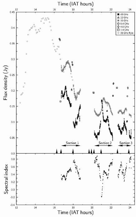
Figure 1: Top panel shows lightcurves of the Ryle observations at 15 GHz (dotted circles) and the VLA observations at 43 GHz (black) and 15 GHz (grey). Also shown are measurements at 22 GHz (hollow triangles), 8.4 GHz (hollow circles), 4.8 GHz (hollow diamonds) and 1.4 GHz (hollow squares). 0 h IAT corresponds to MJD 52299.0. Vertical arrows on the time axis denote times of referenced pointing observations. Bottom panel shows the instantaneous spectral index between 43 and 15 GHz, $\alpha^{15}_{43}$.

The source is in the optically thin decay phase following the flare at $\sim 15$ h, with smaller flares superimposed on this steady decrease in flux density. The amplitude of these events is greater at 43 GHz than at 15 GHz, and they peak 10–15 min earlier at the higher frequency, reminiscent of the behaviour observed in GRS 1915+105 (e.g. Pooley & Fender, 1997; Mirabel et al., 1998; Fender et al., 2002).

2.2 Polarization

With the wide parallactic angle coverage of an 8-hour observation, it was possible to solve for the “D-terms” (the leakage of right circular polarization signal into left circular polarization feeds and vice versa) using the calibrator J 2007+404. Since 3C 286 was resolved by our combination of frequency and array configuration, we used J 2136+006 as a position angle calibrator (assuming a position angle of 26.9° at 43 GHz and 70.0° at 15 GHz, derived from monitoring data taken the following day by NRAO staff). However, the polarization position angle for this source can change by several tens of degrees in two weeks, so the absolute polarization position angles derived (the electric vector position angles; EVPAs) should be treated with caution. Nevertheless, the magnitude of polarization, $P=\sqrt{Q^{2}+U^{2}}$ (where $Q$ and $U$ are the polarized flux densities in the Stokes $Q$ and $U$ parameters) is reliable.

At 15 GHz, no evidence for linear polarization at the source position was seen, down to an r.m.s. level of 0.22 mJy beam^-1 for a single 20-min scan and 0.06 mJy beam^-1 for the full dataset. For a mean 15-GHz flux density of 177.0 mJy, this corresponds to a $5\sigma$ upper limit of 0.17 per cent on the linear polarization. At 43 GHz, however, significant linear polarization was detected, at levels of up to 2.5 mJy. The level of linear polarization initially decreases in line with the total intensity, but then rises during and after the flare at $\sim 21$ h (Fig. 2). No circular polarization was detected at either frequency to a $5\sigma$ limit of 0.6 mJy beam^-1.

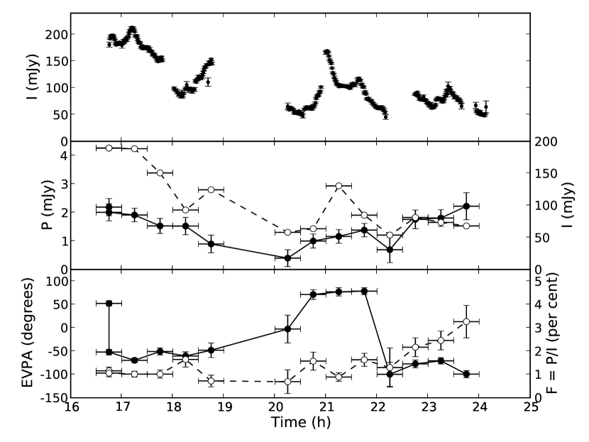
Figure 2: The polarization parameters of Cygnus X-3 at 43 GHz. Top panel shows the full total intensity 43-GHz VLA lightcurve, middle panel shows the total intensity lightcurve binned in half-hour-long intervals (open circles, dashed line, right hand axis) and the linear polarization lightcurve (filled circles, solid line, left hand axis) binned to the same resolution. Bottom panel shows the electric vector position angle (filled circles, solid line, left hand axis) and fractional polarization in per cent (open circles, dashed line, right hand axis) as a function of time. In the lower two panels, the two data points for the first time bin denote the two distinct peaks seen in the polarization image.

Linear polarization has occasionally been detected in previous giant flares of Cyg X-3 (e.g Seaquist et al., 1974; Ledden et al., 1976), up to levels of $\sim 20$ per cent, with the fractional polarization increasing with frequency. However, the majority of observations have shown no significant polarization, with upper limits of a few per cent (e.g. Braes & Miley, 1972; Hjellming & Balick, 1972), so there are relatively few datasets available for comparison. Tudose et al. (2007) used the European VLBI Network (EVN) to resolve polarized emission from Cyg X-3, finding a maximum fractional polarization of 25 per cent at the boundary where an ejected knot was interacting with its environment. For the derived rotation measure (RM) of $-1233$ rad m^-2 (Ledden et al., 1976), we would expect a rotation of $-0.5$ rad at 15 GHz, and $-0.06$ rad at 43 GHz. This RM was derived during giant outbursts, when the emitting regions had propagated further from the core than those we see during these small flaring events. It is likely therefore, that there is some extra Faraday rotation in the inner region, causing depolarization at the lower frequency either due to averaging within the synthesised beam of the observations or along the line of sight. However, since the theoretical maximum fractional polarization for an optically thick source is $\sim 12$ per cent, as compared to $\sim 70$ per cent for an optically thin source, we would in any case expect a lower degree of polarization at 15 GHz, where the optical depth is greater. The beam and line-of-sight depolarization then reduce the observed degree of polarization still further, below our detection threshold.

At 43 GHz, the polarization position angle is stable to within $\sim 20$° except during the flare at $\sim 21$ h, which causes a significant, albeit temporary, rotation of the polarization position angle, while the degree of linear polarization increases slightly. If this flare is due to the formation of internal shocks in the flow (see Section 4), the resulting compression of the magnetic field at the shock front could be responsible for the rotation of the polarization position angle and the increase in polarized intensity. Bearing in mind the uncertainty in absolute position angle calibration, we see the mean EVPA evolve from $-58^{\circ}\pm 10^{\circ}$ at the start of the observations, through $76^{\circ}\pm 4^{\circ}$ during the flare at 21 h, back to $-84^{\circ}\pm 15^{\circ}$ at the end of the observations (as shown in Fig. 2). For optically-thin emission, the measured EVPA should be perpendicular to the magnetic field orientation. Previous high-resolution observations (Mioduszewski et al., 2001; Miller-Jones et al., 2004; Tudose et al., 2007) have shown a north-south jet axis with a position angle close to $0^{\circ}$. Thus a field principally aligned along the jet axis should have an EVPA of $\sim 90^{\circ}$, while compression due to a shock viewed sideways should give an EVPA of $\sim 0^{\circ}$. While the EVPA at the end of the observations is consistent with a field aligned along the jet axis, there are several possible explanations for the intermediate position angles seen earlier. In the absence of precession, either there is additional Faraday rotation beyond the $3^{\circ}$ expected from the previously derived RM, the EVPA calibration is inaccurate, or we are seeing emission from a superposition of emitting regions, some with a longitudinal field configuration (upstream of the shock front), and some from the compressed fields at the shock front. Alternatively, if we are seeing the shock front close to face on, as has been proposed for Cygnus X-3 (Lindfors et al., 2007), owing to the small angle between the jet axis and the line of sight (Mioduszewski et al., 2001; Miller-Jones et al., 2004), we would not expect to see an increase in the degree of ordering of the field. In the absence of data at different frequencies, or at higher spatial and time resolution, it is not possible to differentiate between these competing explanations.

The rise in fractional polarization towards the end of the observation could be explained in part by the expansion of the emitting region following the large flare at the start of the observations. As the source becomes more optically thin, the theoretical maximum fractional polarization increases. Furthermore, the density of the stellar wind of the companion star decreases as the ejecta move outwards, reducing the effect of Faraday depolarization in the wind. Alternatively, a change in the relative dominance of a depolarized core and highly-polarized ejecta, as seen in XTE J 1748-288 (Brocksopp et al., 2007), could be behind the increase in fractional polarization (consistent with the hypothesis of multiple emitting regions proposed to explain the observed EVPAs). Multifrequency data or resolved VLBI observations would be required to test these hypotheses, while higher sensitivity would allow us to make higher-time resolution lightcurves in linear polarization, and more accurately probe how well the polarized emission followed the total intensity. Upcoming facilities such as EVLA and eMERLIN will provide the required increases in sensitivity and fractional bandwidth to make such observations.

2.3 Imaging

Imaging at 43 GHz with the VLA in A-configuration gives an angular resolution of order 50 mas. This would be sufficient to resolve arcsecond-scale extensions such as those seen by Martí et al. (2001), if present during our observations. However, given the time-variable nature of the source, the variability had to be removed prior to imaging the source in order to search for any potential faint extensions. Imaging without removing the variability showed no extension to an r.m.s. level of 1.8 mJy beam^-1. An automated procedure was written using ParselTongue, a Python interface to aips, to remove the time-variable core by making images of 1-min time chunks, and subtracting the fitted core component in the uv-plane before recombining and imaging the core-subtracted data from all time intervals. At 15 GHz, there was no observable extension down to an rms of 0.6 mJy beam^-1. The subtraction did not work as well at 43 GHz, possibly due to atmospheric distortions shifting the source position slightly. The central source was not fully removed, although no evidence for extension was seen down to an rms of 0.2 mJy beam^-1.

The different proper motion measurements quoted in the literature (Mioduszewski et al., 2001; Martí et al., 2001; Miller-Jones et al., 2004) all predict that a flare would take several days to become sufficiently extended to be resolved at 15 GHz by the VLA in its A-configuration. The 400-mJy flare at the start of our observations could not therefore have been resolved. The Ryle Telescope monitoring data show no flares with 15-GHz flux densities exceeding 250 mJy between the 2001 September outburst (Miller-Jones et al., 2004) and the beginning of our observations. The lack of extended emission down to our rms limit of 0.2 mJy then constrains the e-folding time for the decay of any low-level flares to be $<5.2$ d, and that for the 2001 September giant flare to be $<12.5$ d.

2.4 Spectra

The overall radio spectrum was sufficiently well-sampled on four occasions over the course of the January 2002 observing run to generate broadband spectra (Fig. 3).

Figure 3: Broadband radio spectra for the four epochs when the lightcurve was well-sampled. The times (IAT hours relative to MJD 52299.0) of the observations are noted in the bottom left of each plot. Note the turnover moving to lower frequency and flux density with time.

The spectra are consistent with canonical synchrotron spectra affected by absorption at the lower frequencies. The overall flux density decreases with time and the spectral turnover moves to lower frequencies. This is the behaviour expected for the decay of the 400-mJy flare at the start of the observations, as the ejecta move outwards from the core and expand. The lower-level variability seen in Fig. 1 is a secondary effect superposed on the general decrease, indicative of multiple emitting components in the source.

3 Opacity effects

As noted in Section 2.1, the lower-frequency lightcurve is a smoothed and delayed version of the emission at the higher frequency, a clear indication of the existence of opacity effects, as commonly observed in flaring sources such as AGN (e.g. Aller et al., 1985), supernovae (e.g. Weiler et al., 1986), and gamma-ray bursts (e.g. Soderberg et al., 2006). Since the optical depth for both free-free absorption and synchrotron self-absorption decreases with increasing frequency, we probe more compact regions at high frequencies, with lower-frequency emission being delayed until the source has either expanded or moved out from behind the absorbing medium and the optical depth has decreased to order unity.

Molnar et al. (1984) observed similar low-level activity in Cyg X-3 with small flares which peaked later and with smaller amplitudes at lower frequencies. They measured a delay of $15\pm 5$ min between 22 and 15 GHz, increasing to $239\pm 7$ min between 15 and 1.4 GHz. They also claimed evidence for a periodicity in the range 4.8–5.1 h, although such a periodicity has not since been detected (e.g. Johnston et al., 1986, who note that in fact the amplitude of any periodic phenomenon in the data of Molnar et al. is less than 30 mJy). To search for any periodicity in our data, we constructed the power spectra of the lightcurves at the two frequencies, which are shown in Fig. 4.

3.1 Power spectra

Since the data were not evenly sampled in time, in order to construct the true power spectra of the lightcurves, we implemented a one-dimensional version of the CLEAN algorithm, as described by Roberts et al. (1987) and used in standard data reduction procedures for aperture synthesis radio telescopes. We ascertained the significance level of the peaks in the CLEAN spectra by performing Monte Carlo simulations, randomly stripping out half the data points in the time series and calculating the CLEAN spectra using the remaining data (Heslop & Dekkers, 2002). The 95 per cent confidence limit $\alpha_{95}$ was set at the point below which lay 95 per cent of the sorted, concatenated CLEAN spectra from all 1000 Monte Carlo iterations. The final CLEAN spectra of the 43 and 15 GHz data are shown in Fig. 4, together with their respective significance levels $\alpha_{95}$ of 2.1 mJy and 0.67 mJy respectively.

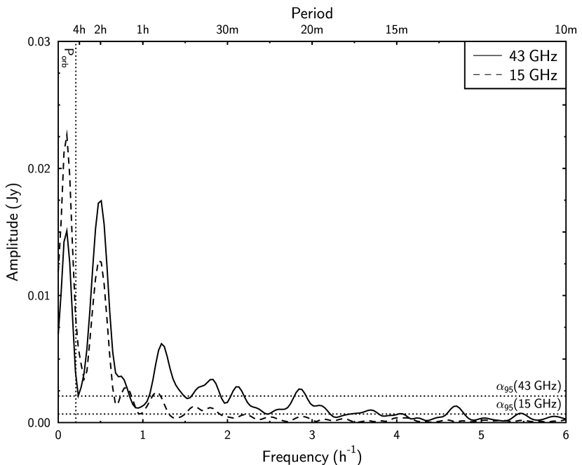
Figure 4: Power spectra of 15- (dashed) and 43-GHz (solid) data. The vertical dotted line shows the 4.8-hour orbital period of the system. The labelled horizontal dotted lines show the 95 per cent significance levels, $\alpha_{95}$, for the 15- and 43-GHz data.

There is no significant power on periods shorter than about 20 min at 43 GHz, and about 30 min at 15 GHz. These minimum variability timescales provide approximate constraints on the size scales for the $\tau=1$ surface of the emitting region at the two frequencies, equal to 2.4 and 3.6 AU respectively (assuming material to be travelling at $c$). At 10 kpc (Dickey, 1983), this corresponds to a size of 0.2–0.3 mas. This may be compared with the predicted scattering size of $448(\nu/1{\rm GHz})^{-2.09}$ mas (Mioduszewski et al., 2001), which equates to 0.2 mas at 43 GHz and 1.6 mas at 15 GHz. At 15 GHz, we are probing regions smaller than can be accessed with VLBI imaging observations.

The power at 15 GHz is uniformly lower than at 43 GHz, owing to the smoothing out of the lower-frequency emission due to the larger size of the emitting region. The most significant peaks in the power spectra correspond to a period of about 2 h at both frequencies. The lowest-frequency peaks correspond to the overall decrease in the mean flux density with time, and are not sampled sufficiently well to correspond to a believable periodicity. There is no significant peak at the orbital period (4.8 h) at either frequency, consistent with the findings of Ogley et al. (2001).

3.2 Delay between the frequencies

To quantify the time delay between the two frequencies, we cross-correlated the lightcurves using the ‘locally-normalised discrete correlation function’ (LNDCF) of Lehár et al. (1992). This accounts for the uneven sampling of the data and the non-stationary nature of the time series, preventing the correlation function from being dominated by interpolations (as is the case for the standard correlation function method) and avoiding the introduction of sampling artifacts (Moles et al., 1986; Peterson, 1993).

The derived cross-correlation function is shown in Fig. 5. It peaks when the 15-GHz emission lags that at 43 GHz by $9.5\pm 1.0$ min, broadly consistent with the $15\pm 5$ min delay between 22 and 15 GHz found by Molnar et al. (1984). Splitting the data into three sections (16.7–18.8 h, 20.2–22.2 h and 22.7–24.2 h UT, as labelled in Fig. 1), the lag was found to decrease with time, from $13.2\pm 1.0$ min in the first section to $7.0\pm 1.0$ min for the final section. The peak in the cross-correlation function also becomes narrower, with a diminishing amplitude with time, as shown in Fig. 5. This is suggestive of decreasing opacity through the flaring sequence, a trend also seen during the multi-flare outburst sequence of 1994 February–March (Fender et al., 1997), and explained as a decreasing amount of entrained thermal material with time over the course of the outburst.

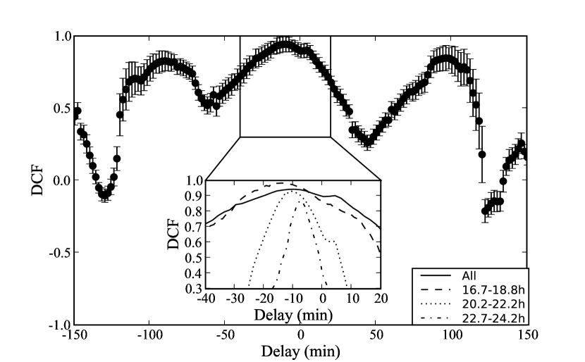
Figure 5: Cross-correlation between the 15-GHz and the 43-GHz lightcurves. Negative delays indicate that the 15-GHz lightcurve lags the 43-GHz lightcurve. Lag bins are of length 2 min. Inset shows the peak of the cross-correlation function for the three different sections of data, plotted without error bars for clarity. The solid line is for the entire data set, the dashed line is for Section 1, the dotted line is for Section 2 and the dot-dashed line is for Section 3.

In an attempt to better understand the relation between the two lightcurves, we now attempt to fit the data with a shock-in-jet model.

4 The shock-in-jet model

Shock-in-jet models have been successfully fitted to the lightcurves of the 1994 outburst of GRO J 1655-40 (Stevens et al., 2003) and to a series of small-scale oscillation events in GRS 1915+105 (Türler et al., 2004). It was suggested that the same model could be used to fit the giant outbursts of the latter source, by simply scaling the timescales, peak flux densities and frequencies of the individual events. Lindfors et al. (2007) applied the shock-in-jet model to Cygnus X-3, finding a good fit to the data from both the 2001 giant outburst and a sequence of intermediate-level flares from 1994. To ascertain whether such a shock model was appropriate to the smaller-scale events we observed in 2002, and to derive some of the physical parameters of the outburst for comparison with the stronger flares seen in this system, we fitted the radio lightcurves with a shock-in-jet model.

4.1 Outline of the model

An analytic model for the evolution of a shock wave propagating down an adiabatically-expanding conical jet was originally derived by Marscher & Gear (1985). This model was generalised by Türler et al. (2000), and further refined for application to microquasar systems by Türler et al. (2004) and Lindfors et al. (2007). According to this model, a shock wave propagating down a jet evolves through three different phases, in which the dominant energy loss mechanism evolves from inverse Compton losses to synchrotron emission, and finally adiabatic expansion. In the inverse Compton stage, the peak emission frequency decreases while the peak flux density rises. Once the photon energy density becomes equal to the magnetic energy density, synchrotron losses take over, and the spectral peak moves to lower frequency at roughly constant flux density. Finally, during the adiabatic phase, both the turnover frequency and flux density decrease with time.

To fit the observed lightcurves with this model, each peak in the lightcurve is associated with the evolution of a single shock front. The fitted start time of an event, $T_{0}$, is the time of onset of the shock, which has been found to correspond fairly closely to the zero-separation time of individual VLBI components in AGN jets (Türler et al., 1999; Lindfors et al., 2006). All shocks are assumed to be self-similar, and the characteristics of an individual event (hereafter referred to as the specificities) are set only by a shift in peak flux density, frequency and duration with respect to the average outburst, to minimize the number of free parameters of the model.

A detailed description of the model is given by Türler et al. (2000), although we have incorporated a number of refinements in fitting the lightcurves presented in Section 2. Björnsson & Aslaksen (2000) modified the shock model to make the rise in flux density in the initial Compton stage less abrupt than was predicted by the original model of Marscher & Gear (1985). With this modification, it was found to be difficult to differentiate the Compton and synchrotron stages (Lindfors et al., 2007), particularly in the absence of high-frequency infrared data, so we omitted the synchrotron stage from our modelling. We assumed a very simple adiabatically-expanding, conical and non-accelerating (constant Doppler-factor) jet. We also assumed a homogeneous synchrotron source, and that all the emission originates from the approaching jet, since Lindfors et al. (2007) found that accounting for the receding jet in this source did not improve the fit to the major and intermediate outbursts of Cygnus X-3, most likely due to the small angle of the flow to the line of sight.

This model differs from a standard plasmon model (van der Laan, 1966) principally by accounting for the rise phase of the flare in which radiative (Compton or synchrotron) losses dominate over adiabatic losses. In this initial radiative phase, the electrons cannot move far from the shock front before losing energy. The thickness of the emission region behind the shock front then varies close to quadratically with the jet radius $R$, with the exact scaling depending on the parameters of the model (Björnsson & Aslaksen, 2000). Thus the volume decreases more rapidly on tracing the emission back to the apex of the jet, and due to the decreased source volume, the flux density at optically thin frequencies (in the infrared) does not become excessively high at small radii. While we have no simultaneous infrared data from 2002 January 25, and cannot mandate the use of a shock model as opposed to a plasmon model, application of this shock-in-jet model to previous outbursts of Cygnus X-3 (Lindfors et al., 2007) and to GRS 1915+105 (Türler et al., 2004) has shown that it can reproduce both the infrared and radio lightcurves. The second main difference is that since the shock-in-jet model involves an underlying flow expanding in two dimensions, the electron energy decreases more slowly with time, as $E\propto R^{-2/3}$ rather than the $R^{-1}$ scaling expected for a three-dimensional expansion of a discrete plasmon with no turbulence. This in turn leads to a slightly less steep decay of the synchrotron self-absorption turnover flux density with frequency and time.

4.2 Fitting the lightcurves

The radio lightcurves were decomposed into a series of 10 individual events (each representing the development and propagation of a shock within the flow), plus an initial decaying outburst representing residual emission from events prior to the start of the observing period. All frequencies were fit simultaneously to determine both the profile of the average outburst and the logarithmic shifts in flux density ($\Delta\log S$), frequency ($\Delta\log\nu$) and time ($\Delta\log t$) of the transition from the Compton to the adiabatic stage, which determine the specificities of the individual events. It was found that in the absence of infrared data to constrain the high-frequency emission, there was significant degeneracy along the adiabatic evolution track. To discriminate between different weakly-constrained solutions for the specificities of individual outbursts, an extra constraint was placed on the fit parameters, minimizing the combined scatter in the specificities $\Delta\log S$, $\Delta\log\nu$ and $\Delta\log t$. The model used 51 free parameters (seven to specify the shape and evolution of the average event profile, four to represent residual decaying emission at the start of the observations, plus four per outburst to determine the characteristics of each of the ten individual events), fitted to 700 data points. The best fitting model, giving a reduced $\chi^{2}$ of 20.5 for the entire dataset, is shown for the different observing frequencies in Fig. 6. The converged model parameters are given in Table 1, and the derived start times and logarithmic shifts of the different events are listed in Table 2.

Parameter	Value
$s$	2.11
$b$	1.19
$t_{\rm p}$ (h)	0.47
$\nu_{\rm p}$ (GHz)	26.9
$S_{\rm p}$ (Jy)	0.14
$\nu_{\rm b}$ (THz)	$2.30$
$t_{\rm f}$ (h)	0.11

Table 1: The seven model parameters specifying the shape of the average outburst. $s$ is the index of the electron energy spectrum, $b$ is the scaling of the magnetic field with distance $z$ along the jet ($B\propto z^{-b}$), $S_{\rm p}$ is the peak flux density at the transition to the adiabatic stage, $\nu_{\rm p}$ is the frequency at which the flux density peaks, and $t_{\rm p}$ is the time of the peak relative to the onset of the shock at time $T_{0}$. $\nu_{\rm b}$ is the frequency of the high-frequency break in the spectrum where it steepens from $\nu^{-(s-1)/2}$ to $\nu^{-s/2}$, defined at the time of the peak, and $t_{\rm f}$ is the time at which the spectrum begins to flatten to $\nu^{-(s-1)/2}$ prior to the start of the adiabatic stage.

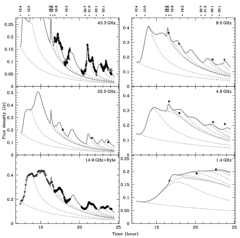
Figure 6: Best-fitting model lightcurves at each frequency, with the data overplotted as open circles. The 15-GHz Ryle Telescope flux densities have been multiplied by a factor 1.25 to bring them into agreement with the 14.9-GHz VLA data. The different outburst events are shown by dotted lines. The frequency of each lightcurve is marked in the top right of each panel. The IAT start times of the different outbursts are indicated by arrows at the top of the figure.

While inspection of Fig. 6 shows that the model appears to reproduce the overall shape of the lightcurves fairly well at 15 and 43 GHz, the reduced $\chi^{2}$ for the overall fit is relatively high. It is possible that the error bars on the data points may have been slightly underestimated. The uncertainties on the data are mainly statistical, although some extra systematic errors of 1 per cent were added to the Ryle Telescope data and the lower-frequency VLA data. However, they do not account for the 3–5 per cent uncertainty in the absolute flux scale at the VLA, since an overall gain error should affect all data points at a given frequency and have no effect on the relative shape of the lightcurves, whereas the discrepancies between the model and the data are in the fine details of the lightcurves rather than their overall normalisations. It is more likely that at these high frequencies, atmospheric variations on a timescale shorter than the switching time between calibrator and target caused extra scatter in the observed flux density.

However, the high reduced $\chi^{2}$ value also reflects the fact that the model is a fairly simplistic idealisation, which does not attempt to reproduce in detail the exact shapes of individual events, and so is unlikely to be able to account for all features of the observed lightcurves. We assumed a conical jet, a strong shock, no reverse shock, and did not account for counter-jet emission or jet precession. The slope of the electron spectrum $s$ was assumed to be constant with time, and the ratio, $\nu_{\rm p}/\nu_{\rm b}$, of the peak frequency to the high-frequency break of the optically-thin synchrotron spectrum was assumed to be the same for all outbursts (albeit evolving with time within an individual event). Real magnetohydrodynamical jets are likely to be far more complicated, with phenomena such as transverse shocks, stationary knots, and Kelvin-Helmholtz instabilities, which we cannot begin to account for in our self-similar analytic model. The fit is clearly sufficient to validate the zero-order picture of adiabatically-expanding synchrotron plasma, although in the absence of high-frequency millimetre or infrared data, discriminating between the rise phases of a shock-in-jet model and a plasmon model is more difficult, and deriving the details of any shock structure is clearly impossible without detailed high-resolution VLBI imaging.

While the electron energy decays more slowly with radius in the shock-in-jet model, the addition of turbulence into the plasma in a plasmon model can slow the decay of the flux density as the plasmon expands. We can examine the expected synchrotron flux density during the adiabatic decay phase for the two different models (e.g. Longair, 1994),

$$S_{\nu}\propto R^{3}\kappa B^{(s+1)/2}\nu^{-(s-1)/2},$$ (1)

where $\kappa$ is the normalisation of the electron spectrum, $N(E)\propto\kappa E^{-s}$, and $B$ is the magnetic field strength. For the shock-in-jet model, $B\propto R^{-b}$ and $\kappa\propto R^{-2(s+2)/3}$. Thus, for the shock-in-jet model,

$$S_{\nu}\propto R^{[10-4s-3b(s+1)]/6}\nu^{-(s-1)/2}.$$ (2)

From the values in Table 1, this scales as $S_{\nu}\propto R^{-1.59}$. For the plasmon model, $B\propto R^{-2+\eta}$, where $\eta$ is a factor describing the degree of turbulence in the plasma, typically of order 1, with $\eta=0$ corresponding to no strong turbulence (Landau & Lifshitz, 1963). The first adiabatic invariant, $p_{\perp}^{2}/B$, is conserved during the expansion, where $p_{\perp}$ is the component of the particle momentum, $p=E/c$, perpendicular to the magnetic field. If the particle distribution is isotropic throughout the expansion, then $p_{\perp}^{2}=2p^{2}/3$, such that $E\propto R^{(-2+\eta)/2}$. Assuming the number of particles in a plasmon, $VN(E)\,{\rm d}E=V\kappa E^{-s}\,{\rm d}E$, is conserved, we then find that $\kappa\propto R^{-[2+s+\eta(1-s)/2]}$, such that

$$S_{\nu}\propto R^{s(\eta-2)}\nu^{-(s-1)/2}.$$ (3)

For the same value of $s$ as fitted for the shock-in-jet model, a value $\eta=1.24$ would then provide the same scaling during the decay phase. Thus we cannot use the decay phases of the outbursts to conclusively discriminate between the two classes of model. Higher-time resolution polarization data would help to discriminate between the two types of flow, since the compression and consequent ordering of the magnetic field at the shock front at the onset of an event would lead to a higher degree of polarized emission and a rotation of the mean position angle of the field, from one aligned parallel to the jet to one aligned perpendicular to it (Hughes et al., 1989a). While there are hints of a rotation of the EVPA during the flare at 21 h (Fig. 2), the fractional polarization does not increase significantly, and higher time resolution (i.e. higher sensitivity) would be required to verify this signature of a propagating shock front.

Nevertheless, owing to the good overall match to the shape of the lightcurves, we will assume that the basic zero-order properties of this model are correct, and go on to use the fitted model parameters to constrain the differences between the 2002 events and the previously-studied outburst sequences of 1994 and 2001.

The shape of the fitted average outburst in the three-dimensional parameter space defined by peak flux density, frequency and time after onset is shown in Fig. 7. Also shown are the locations of the peaks of the individual outbursts, calculated from the average outburst values and the logarithmic shifts in time, frequency and flux density of the individual events (given in Table 2). While there is significant scatter in flux density, they are well-aligned in the frequency-time plane along the locus of the spectral turnover (Fig. 7), suggesting that the turnover always follows a similar track in frequency and time. The scatter in flux density suggests that another factor is at work in determining the brightness of a given outburst, possibly the normalisation of the electron spectrum, $\kappa$. Such an anticorrelation between frequency and timescale has been previously noted in 3C 273 (Türler, Courvoisier & Paltani 1999) and Cygnus X-3 (Lindfors et al., 2007), but not in 3C 279 (Lindfors et al., 2006).

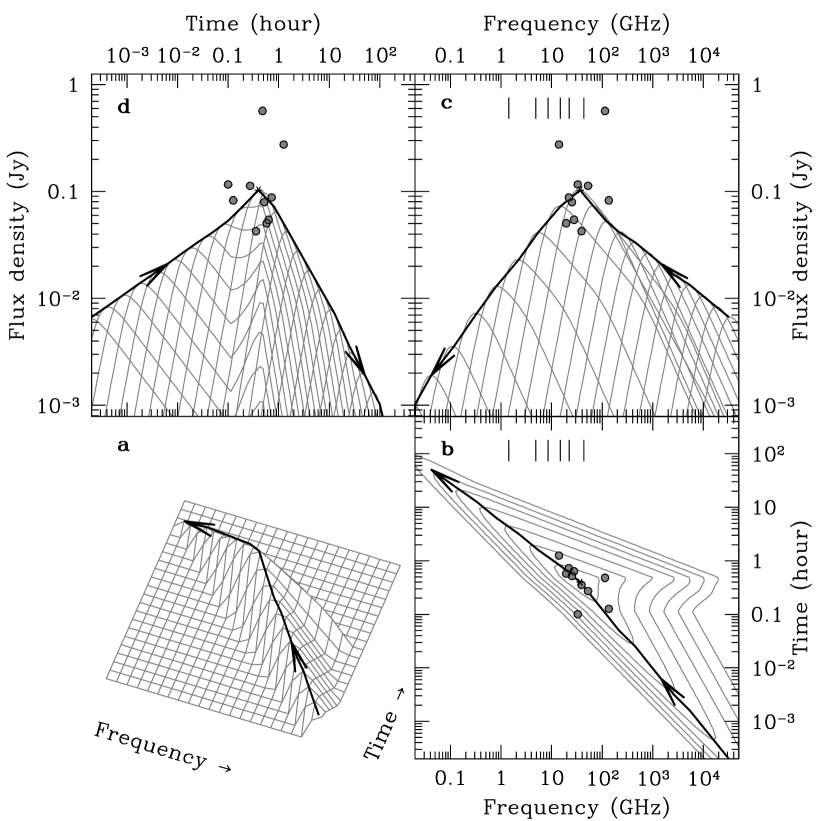
Figure 7: The evolution of the average outburst in frequency-time-flux density space. (a) indicates the path followed by the self-absorption turnover, and (b), (c) and (d) show the projections onto the frequency-time, frequency-flux density and time-flux density axes respectively. The contours in (b) are points of equal flux density, spaced by 0.3 dex. In (c), the grey lines show individual spectra at times spaced by 0.3 dex. In (d), they show lightcurves spaced by 0.3 dex in frequency. The thick black lines show the path followed by the self-absorption turnover, and the grey dots show the time, flux density and frequency of the peak emission of the individual outbursts, each of which is represented by a self-similar scaling of the average outburst. The vertical black lines at the top of (b) and (c) show the observing frequencies. The two outlying points in (c) and (d) are the two earliest flares (starting at 12.38 and 13.47 h respectively), which are constrained only by the Ryle Telescope data and the later low-frequency points.

Epoch	$T_{0}$	$\Delta\log S$	$\Delta\log\nu$	$\Delta\log t$
1994	2.95 d	1.53	-0.59	1.58
	5.80 d	0.92	-0.65	1.62
	7.25 d	0.73	-0.16	1.55
	9.06 d	0.53	-0.29	2.18
	11.44 d	0.66	-0.94	1.18
	12.31 d	1.35	-0.62	1.13
	14.16 d	0.92	-1.28	1.75
	16.19 d	1.33	-0.72	1.06
	18.53 d	0.92	-0.94	1.94
	20.37 d	1.65	-0.87	1.14
	22.89 d	0.90	-1.15	1.63
	23.72 d	1.20	-1.28	1.97
	30.09 d	0.50	-0.66	1.43
2001	2.64 d	1.98	-0.76	1.76
	4.51 d	1.80	-1.14	1.94
	4.64 d	1.70	-0.73	1.78
2002	12.38 h	0.43	-0.42	0.50
	13.47 h	0.74	0.49	0.08
	16.21 h	0.05	-0.04	-0.60
	16.59 h	-0.10	0.57	-0.50
	16.88 h	-0.11	-0.16	0.11
	18.31 h	-0.07	-0.22	0.26
	20.71 h	0.04	0.16	-0.17
	21.24 h	-0.39	0.03	-0.05
	22.13 h	-0.28	-0.12	0.20
	23.06 h	-0.31	-0.28	0.16

Table 2: The fitted start times and logarithmic shifts in flux density, frequency and time, for the three outbursts of Cyg X-3, quoted relative to the average outburst derived for the 2002 dataset.

4.3 Comparison to previous outbursts

A similar shock model was used by Lindfors et al. (2007) to fit the lightcurves of the 1994 February-March and 2001 September outburst sequences of Cygnus X-3. Both flaring sequences were significantly brighter than the events observed in this paper. In order to make valid comparisons between the different outbursts, we re-fitted those datasets using the average outburst and model parameters found from the 2002 January 25 dataset. This provided consistent specificities for the individual outbursts of the different flaring sequences. The new logarithmic shifts, which gave reduced-$\chi^{2}$ values for the 1994 and 2001 datasets of 11.8 and 3.0 respectively (as compared to values of 10.2 and 1.8 from the original fits by Lindfors et al., 2007), are given in Table 2. We note that the sparse infrared data from the 1994 outburst sequence were not well fitted by these model parameters, since there were no infrared data available in 2002 to constrain the high-frequency spectral evolution. However, since our goal was to compare the radio emission from different outbursts in a consistent fashion, we used the average outburst derived from the 2002 data to fit all three flaring sequences, owing to the simplicity of the model (an adiabatically-expanding conical jet, following the original assumptions of Marscher & Gear, 1985).

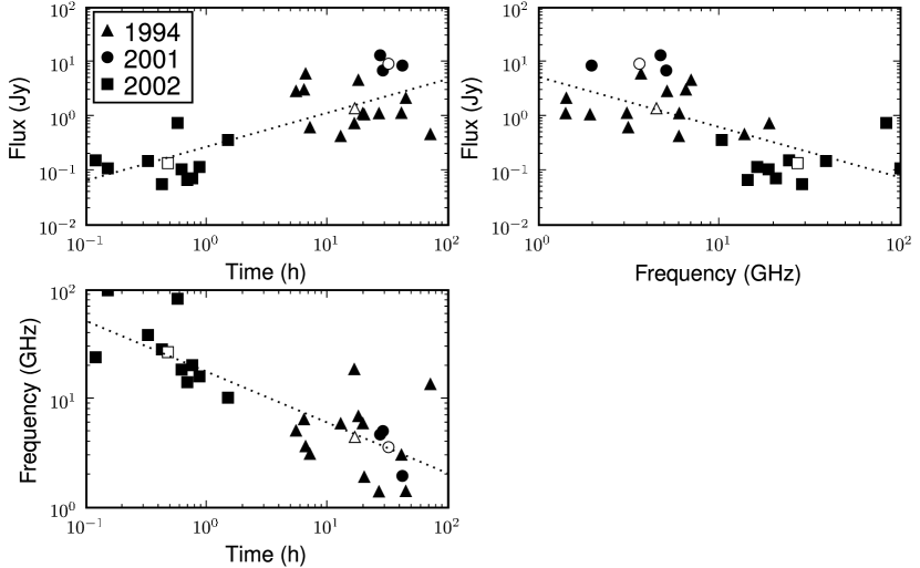
Figure 8: Peak flux density, frequency and time after onset of the shock, for each of the individual outbursts of Cygnus X-3 in 1994 (filled triangles), 2001 (filled circles) and 2002 (filled squares), plotted against one another. The open markers denote the position of the average outburst for each dataset. The dotted lines show the least-squares fits for the scaling of the different parameters with one another; $S_{\rm p}\propto t_{\rm p}^{0.62}$, $S_{\rm p}\propto\nu_{\rm p}^{-0.93}$, and $\nu_{\rm p}\propto t_{\rm p}^{-0.47}$.

In Fig. 8, we use the specificities of the individual outbursts (Table 2) to plot the times, frequencies and flux densities of the peak emission against one another for all three datasets. The peak frequency is anticorrelated with the outburst timescale, not just for the 2002 data, but also between the different outburst sequences. Events that evolve faster peak at higher frequencies (the calculated Spearman rank correlation coefficient is $-0.79$, chance probability $<2\times 10^{-6}$), as found by Lindfors et al. (2007). The timescale of the outburst also shows a positive correlation with the peak flux density (correlation coefficient 0.69, chance probability $<10^{-4}$), and there is an anticorrelation between the peak frequency and peak flux density (correlation coefficient $-0.68$, chance probability $<2\times 10^{-4}$). Thus the shorter, higher-frequency-peaking outbursts also tend to be fainter. Fitted scalings of the three parameters $S_{\rm p}$, $\nu_{\rm p}$ and $t_{\rm p}$ with one another are given in Table 3.

The frequency-timescale correlation could potentially be explained by travel time arguments. If the time of peak emission is related by travel time to the distance from the jet base, then events occurring closer to the core peak earlier and, since they have expanded less, do so at higher frequencies. Self-similar expansion implies that these events evolve fastest.

4.4 Physical parameters

Assuming that the time of peak flux density can be approximated by travel time down the jet, this occurs at a distance $z_{\rm p}=\gamma\beta\delta ct_{\rm p}$ downstream, at which point the jet radius is $R_{\rm p}=z_{\rm p}\tan\phi$ (assuming a cone opening angle of $\phi=2$° in all cases). The source angular size is given by $\theta_{\rm src}=2R_{\rm p}/d$, where $d$ is the source distance (taken to be 10 kpc for Cyg X-3; Dickey, 1983). Given the angular size $\theta_{\rm src}$, turnover frequency, $\nu_{\rm p}$, and flux density, $S_{\rm p}$, and the electron index $s$, with the assumption of a homogeneous spherical source with a power-law electron energy spectrum, then the magnetic field $B$, and the normalisation of the electron spectrum, $\kappa$, can be calculated at the turnover using the equations of Marscher (1987), as previously done for a sample of Galactic and AGN jets by Türler & Lindfors (2007). While for a shock-in-jet model the source has a cylindrical slab-like geometry rather than being spherical, the depth scales with $R$ during the self-similar adiabatic phase, so approximating the source as a sphere will be in error by the ratio of the slab thickness $x$ to the jet radius $R$, a factor $\xi\sim 0.005h^{-5}$ (as derived for the case of 3C 273; Marscher & Gear, 1985), where $h=H_{0}/(100{\rm\,km\,s}^{-1}{\rm\,Mpc}^{-1})$ and $H_{0}$ is the Hubble constant. For the currently-accepted value of $h=0.732$ (Spergel et al., 2007), $\xi\sim 0.024$. Marscher & Gear (1985) also approximated the density of the shocked region as being constant up to a distance $x=\xi R$ behind the shock front, at which point it would abruptly drop to zero. They found that this should not introduce significant errors into the proportionalities for their equations. The assumption of homogeneity of the emitting region was further justified by Björnsson & Aslaksen (2000), and should certainly be sufficient to derive the scalings between physical parameters which we now present. Adapting the equations of Marscher (1987) to account for the non-spherical geometry, and assuming we see the emitting region with the shock face-on (Lindfors et al., 2007), the magnetic field is given by

$$B_{\rm p}=10^{-5}b(\alpha)\theta_{\rm src}^{4}\nu_{\rm p}^{5}S_{\rm p}^{-2}\delta\quad{\rm G},$$ (4)

the electron normalisation is

$$\kappa_{\rm p}=10^{6}n(\alpha)d^{-1}\xi^{-1}\theta_{\rm src}^{-(4\alpha+7)}\nu_{\rm p}^{-(4\alpha+5)}S_{\rm p}^{2\alpha+3}\\ \times\delta^{-2(\alpha+2)}{\rm erg}^{2\alpha}{\rm cm}^{-3},$$ (5)

and the optical depth to synchrotron self-absorption at the turnover frequency is

$$\tau_{\rm p}(\alpha)=c_{2}(\alpha)\kappa_{\rm p}B_{\rm p}^{(3+2\alpha)/2}\nu_{\rm p}^{-(5+2\alpha)/2}\xi\theta_{\rm src}d\delta^{(5+2\alpha)/2},$$ (6)

where the source size $\theta_{\rm src}$ is given in mas, the peak emission frequency $\nu_{\rm p}$ in GHz, the peak flux density $S_{\rm p}$ in Jy and the source distance $d$ in kpc. $\alpha=(s-1)/2$ is the spectral index, and $n(\alpha)$ and $c_{2}(\alpha)$ are functions depending logarithmically on $\alpha$, with values of 0.27 and $1.2\times 10^{17}$ respectively for $\alpha=0.5$. $b(\alpha)$ is a slowly-varying function of $\alpha$ with a value of 3.2 for $\alpha=0.5$. Away from the peak, the optical depth scales with frequency as $\tau\propto\nu^{-(2\alpha+5)/2}$.

To meaningfully compare the physical parameters for different outbursts, they should be scaled to the same position $z$ along the jet (i.e. to a fixed jet radius $R$). The magnetic field and electron normalisation scale as power laws with jet radius, $B\propto R^{-b}$ and $\kappa\propto R^{-k}$. $b$ is given in Table 1, and $k=2(s+2)/3$ for an adiabatic jet flow as assumed here. From the peak fluxes, frequencies and times of the individual outbursts, the magnetic field, electron normalisation, and optical depth to synchrotron self-absorption at a frequency of 15 GHz were calculated, scaled to the same jet radius of 1 AU using the derived values of $b$ and $k$, and plotted against peak flux density, $S_{\rm p}$, frequency, $\nu_{\rm p}$, and time, $t_{\rm p}$ in Fig. 9. In all cases we assumed a distance of 10 kpc (Dickey, 1983), a jet speed $\beta=0.63$, an inclination angle of 10.5° to the line of sight and a jet half-opening angle of 2°(Miller-Jones et al., 2004). While we note that slightly different parameters were found by Mioduszewski et al. (2001), we use a single set of parameters here for consistency between outbursts.

	$S_{\rm p}$	$\nu_{\rm p}$	$t_{\rm p}$	$B(1{\rm AU})$	$\kappa(1{\rm AU})$	$\tau(1{\rm AU})$
$S_{\rm p}$		-0.46	0.91	[0.38]	1.58	2.40
$\nu_{\rm p}$	-0.93		-1.36	[-0.19]	-2.23	-2.64
$t_{\rm p}$	0.62	-0.47		1.61	[-0.55]	2.85

Table 3: Fitted scalings of the peak turnover flux density $S_{\rm p}$, frequency $\nu_{\rm p}$ and time $t_{\rm p}$ with one another and the resulting predictions, via equations 4, 5, and 6, for the scaling of the magnetic field, electron normalisation, and optical depth at 15 GHz to synchrotron self-absorption, normalized to 1 AU, with the three parameters $S_{\rm p}$, $\nu_{\rm p}$ and $t_{\rm p}$. The numbers are the power-law index to which the parameter in the relevant row is raised to give the scaling of the parameter in the selected column, such that, for instance, $S_{\rm p}\propto\nu_{\rm p}^{-0.93}$. Correlations which a Spearman rank test show not to be significant at the 95 per cent level are shown in brackets.

There is clearly significant scatter in the individual events (due to the strong dependences of $B$ and $\kappa$ on $S_{\rm p}$, $\nu_{\rm p}$ and $\theta_{\rm src}$). However, we can use equations 4, 5 and 6 together with the derived scalings of $S_{\rm p}$, $\nu_{\rm p}$ and $t_{\rm p}$ with one another, given in Table 3, to show the expected trends in $B$, $\kappa$ and $\tau$. These are plotted as dashed lines in Fig. 9. Spearman rank correlations show that the only significant trends are for the magnetic field to increase with event duration (correlation coefficient 0.64, chance probability $4\times 10^{-4}$), the electron normalisation to increase with event brightness (correlation coefficient 0.47, chance probability 0.015) and decrease with peak frequency (correlation coefficient 0.47, chance probability 0.034), and for the opacity to increase with brightness and duration, and to decrease with frequency. The correlations which are not found to be significant have the shallowest power law indices (between $-1.0$ and $1.0$), suggesting that they are the most easily masked by the scatter in the parameters. The correlation of optical depth with event parameters is due to the distance along the jet at which the peak occurs. The shorter outbursts peak at higher frequencies and closer to the core, and have already reached their peak flux density at 15 GHz by the time the jet reaches a radius of 1 AU, so they are optically thin. The large, bright outbursts have not yet expanded sufficiently to become optically thin at 15 GHz by the time the jet radius is 1 AU. The calculated values for the physical parameters of the average outbursts of 1994, 2001 and 2002 are listed in Table 4. With the derived magnetic field strengths, the synchrotron loss timescales at 43 GHz range from 18 d to 70 y. By the time the shock has reached the radio photosphere, its size is not limited by radiative losses, having instead been set earlier when the magnetic field was higher, since when it has been determined by adiabatic expansion. Thus we cannot further constrain the size of the emitting region using the radiative loss timescale.

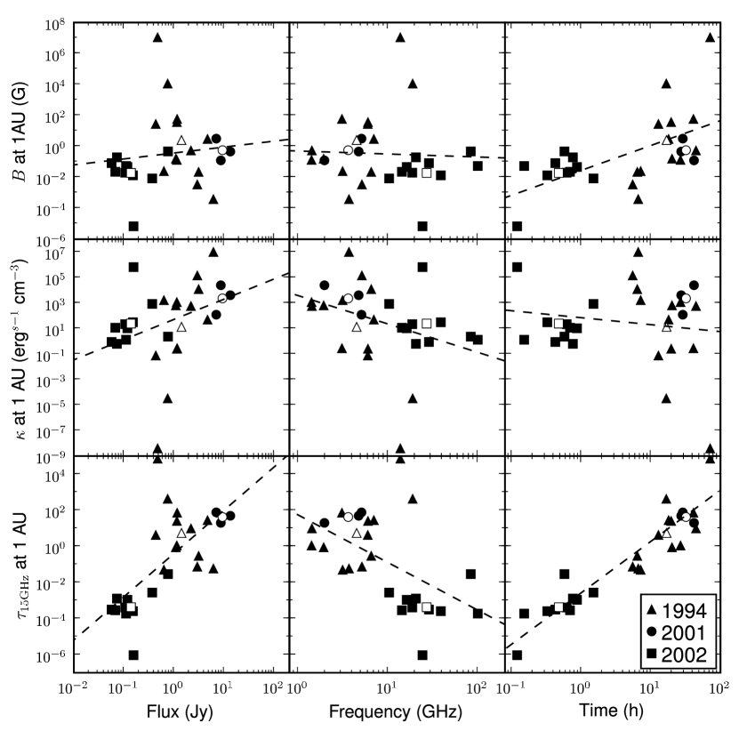
Figure 9: Magnetic field (upper panels), electron normalisation (middle panels), and 15-GHz optical depth to synchrotron self-absorption (lower panels) scaled to a jet radius of 1 AU, and plotted against peak flux density, frequency and time for each of the individual outbursts of Cygnus X-3 in 1994 (filled triangles), 2001 (filled circles) and 2002 (filled squares), together with the average outburst properties for each of the three flaring sequences (open symbols). The dashed lines show the predictions for the scalings of the different parameters with flux, frequency, and time, according to the fitted coefficients shown in Table 3.

Parameter	1994	2001	2002
$<S_{\rm p}>$ (Jy)	1.4	9.3	0.14
$<\nu_{\rm p}>$ (GHz)	4.5	3.6	26.9
$<t_{\rm p}>$ (h)	16.8	31.9	0.47
$z_{\rm p}$ (AU)	201	381	5.7
$R_{\rm p}$ (AU)	7.0	13.3	0.20
$B_{\rm p}$ (G)	0.25	0.03	0.13
$B(1{\rm AU})$ (G)	2.54	0.56	0.02
$\kappa_{\rm p}$ (ergs-1cm-3)	$6.5\times 10^{-2}$	$1.9\times 10^{0}$	$2.1\times 10^{3}$
$\kappa(1{\rm AU})$ (ergs-1cm-3)	$1.4\times 10^{1}$	$2.3\times 10^{3}$	$2.5\times 10^{1}$
$\tau_{\rm p}(15{\rm GHz})$	$1.6\times 10^{-3}$	$8.2\times 10^{-4}$	$3.8\times 10^{-1}$
$\tau(1{\rm AU})(15{\rm GHz})$	$5.6\times 10^{0}$	$4.3\times 10^{1}$	$4.3\times 10^{-4}$

Table 4: A comparison of the fitted parameters of the different outbursts of Cygnus X-3 (2002 January 25 from this paper, and 2001 September and 1994 February-March from Lindfors et al., 2007), and the physical quantities derived from them. For a given flaring sequence, the average time, frequency and flux density of the peak in the spectrum are $<S_{\rm p}>$, $<\nu_{\rm p}>$ and $<t_{\rm p}>$. This occurs at the transition from the Compton to the adiabatic stage, a distance $z_{\rm p}$ downstream in the jet where the jet radius is $R_{\rm p}$. At this point, the magnetic field is $B_{\rm p}(S_{\rm p},\nu_{\rm p},t_{\rm p})$, the electron normalisation is $\kappa_{\rm p}(S_{\rm p},\nu_{\rm p},t_{\rm p})$, and the optical depth to synchrotron self-absorption at 15 GHz is $\tau_{\rm p}(S_{\rm p},\nu_{\rm p},t_{\rm p})$(15 GHz). Extrapolating these last three values back to the point where the jet radius is 1 AU, for valid comparison between the flaring sequences, gives the magnetic field $B(1{\rm AU})$, the electron normalisation $\kappa(1{\rm AU})$ and the optical depth $\tau(1{\rm AU}$)(15 GHz).

To investigate the decreasing opacity over the course of the flare sequence suggested by Fender et al. (1997) and seen in our analysis in Section 3, we performed a Spearman rank-order correlation test between the start times of the individual outbursts of 2002 January 25 and their peak flux densities, frequencies and timescales shown in Table 2. The only significant correlation was a trend for the peak flux density to decrease with start time, with a Spearman rank coefficient of $-0.83$ ($<0.3$ per cent probability of a chance correlation). This trend, due to the decay of the flare at the start of the observations, is seen in the individual lightcurves of Fig. 1. There was no significant correlation of optical depth with start time. If the opacity is indeed decreasing over the course of a flaring sequence, that opacity is not generated by the synchrotron mechanism. It could be free-free absorption due to a decreasing proportion of entrained thermal material (Fender et al., 1997), although such a component was not included in our modelling, so its effects cannot be quantified. We would need simultaneous well-sampled lightcurves at lower frequencies to investigate its effects.

4.5 The differences between large and small outbursts

VLBI observations (Mioduszewski et al., 2001; Miller-Jones et al., 2004; Tudose et al., 2007) have clearly demonstrated that the outbursts of Cygnus X-3 vary in jet morphology as well as in strength, showing both one-sided and two-sided jets, with the dominant component moving to the south in some cases and to the north in others. Such differences cannot be explained by varying the magnetic field strength or electron normalisation at the onset of the shocks. Changes in the accretion flow, or in the immediate environment of the binary system, possibly due to changes in the strength of the stellar wind, are plausible explanations for such variations in the jet morphology. However, bearing such caveats in mind, we can attempt to use our jet model fits to gain some insight into the differences between large and small outbursts. Varying the jet orientation and environmental parameters will add scatter to the observed relations, but we can hope to discern general trends.

We found that the same shock-in-jet model can explain the radio lightcurves of Cygnus X-3 during giant outbursts, intermediate flares, and low-level activity, suggesting that the three discrete variability classes identified by Waltman et al. (1994) are similar phenomena, which differ only in scale. This indicates that a jet outflow persists into the low-level active state in which Cygnus X-3 spends the majority of its time, and that the formation of shocks is responsible for the observed events in the radio lightcurves. Outbursts which peak earlier do so at higher frequencies and with lower peak flux densities. The fitted model parameters strongly suggest that the faster, weaker outbursts occur closer to the core, whereas the brighter outbursts occur further downstream. For a constant jet speed (as assumed in our modelling), this implies that shocks forming further downstream take longer to expand by a given factor, giving rise to a longer timescale for the emission, and a lower peak frequency.

While Fig. 9 has considerable scatter, as expected from the above discussion, the observed trends demonstrate that the brighter, lower-frequency peaking outbursts have higher electron normalisations. The trends with magnetic field are not as clear-cut, although the correlation of longer-duration outbursts with magnetic field suggests that the brighter, lower-frequency peaking outbursts should also have higher magnetic field strengths. It is possible that the shallowness of these correlations allow them to be masked by the scatter in the parameters, making them appear less significant. If both the magnetic field and electron normalisation are higher for stronger outbursts, it suggests that some significant fraction of the magnetic field could be generated by the electrons themselves. However, the dependences of the observable parameters $S_{\rm p}$, $\nu_{\rm p}$ and $t_{\rm p}$ on the underlying physical parameters $B$ and $\kappa$ are clearly complex, and better modelling is required to disentangle the relative importance of the magnetic field and electron normalisation in determining the size of the outbursts.

4.6 Implications for high-resolution imaging

While the lightcurves can be well fitted by shocks propagating down a jet, it is natural to consider whether these events in fact correspond to discrete VLBI components. Hughes, Aller & Aller (1989b, 1991) found that a model consisting of shocks propagating down a jet could explain the observed evolution of the total intensity, polarized intensity, and VLBI morphology of three extragalactic radio sources.

Several studies (e.g. Mutel et al., 1990; Abraham et al., 1996) have found that peaks in total intensity lightcurves correspond to the ejection of new VLBI components, with the flux density of the ejected components roughly corresponding to the increase in total flux density. Subsequently, the decomposition of lightcurves into discrete flaring events (Valtaoja et al., 1999; Türler et al., 1999; Lindfors et al., 2006) has found a good correspondence between VLBI component zero-separation dates and the fitted start times of those events. However, the component flux densities were less well fitted, probably due to an underestimate by the model of the contribution of the underlying jet. The largest sample studied to date, incorporating 27 blazars, found that every resolved VLBI component had a corresponding flare in the total intensity lightcurve, with zero-separation dates which corresponded well to the start dates of the flares inferred from the lightcurves (Savolainen et al., 2002). But again, while the flux densities of the flares correlated with those of the resolved VLBI components, there was significant scatter about this relation.

Flares in the total flux density are also observed which do not appear to correspond to resolved ejecta on VLBI scales (e.g. Pyatunina et al., 2006; Lindfors et al., 2006). The favoured explanation (reinforced by evidence for unresolved components derived from a closure phase analysis performed by Savolainen et al., 2002) is that such events do produce ejecta, but that these have faded before propagating out to the point where they can be resolved. Savolainen et al. (2002) therefore suggested that every large ($>30$ per cent increase in flux density) flare in the total intensity lightcurve corresponded to the formation of a new shock. This raises the question of what sets the decay time of the ejecta. If the shock takes a long time to become optically thin at the observing frequency, the emission will have faded before it can propagate out far enough to be resolved. Similarly, if there are significant radiative losses (particularly important at higher frequencies), the emission will rapidly fade below the detection limit. In our model, the location of the outburst in the three-dimensional frequency-time-flux density space will then determine whether or not a given flare fades too rapidly to be resolved at the observing frequency. We note however, that the model is an oversimplification, and that other events such as instabilities in the flow, magnetic field enhancements, or interaction with the surroundings could cause a rebrightening further downstream, allowing components that would not otherwise be resolved to be detected. While we cannot hope to account for such phenomena without introducing many extra free parameters while attempting to model the observed lightcurves, they could help to account for the discrepancies between model predictions and VLBI observations.

In the case of Cygnus X-3, VLBI jets have been seen out to angular distances of 50–100 mas (Mioduszewski et al., 2001; Miller-Jones et al., 2004; Tudose et al., 2007). Since the peak frequency $\nu_{\rm p}$ scales with distance (i.e. time) along the jet as $z_{\rm p}^{-0.47}$ (Table 3), the low-level flares seen here, with peak frequencies ten times lower than those seen in the giant flare of 2001, might be expected to be extended at the 10–20 mas level, assuming that the speeds of propagation were similar in both cases. However, the resolved knots seen during giant flares were observed well after the peak of the outbursts, while the emission was fading. For an outburst peaking at flux densities 100 times lower, it would be challenging to detect extension at such low levels. Furthermore, travel-time arguments suggest that it would take several hours for shocks travelling at $c$ to reach angular distances of 10–20 mas, for a source distance of 10 kpc. Indeed, the constraints on the source sizes derived in Section 3 were 0.2–0.3 mas, smaller than the scattering disk and at the limit of what can be achieved with current VLBI arrays, even at the highest frequencies. We therefore find it unlikely that these flaring events could be resolved with current instrumentation.

5 Absorption mechanisms

In Section 3, we quantified the opacity effects which led to the delay and smoothing of the 15-GHz lightcurve with respect to that at 43 GHz. However, the nature of such opacity was not explicitly determined. Plausible absorption mechanisms are synchrotron self-absorption (Mirabel et al., 1998), and free-free absorption from either the wind of the companion star (e.g. Fender et al., 1995; Waltman et al., 1996), or from entrained thermal electrons in the jet (Fender et al., 1997).

We can quantify the effect of the dense wind of the Wolf-Rayet companion star, which causes delays as the emitting regions move out from behind the radio photospheres, located closer to the central binary at higher frequencies. Using the parameters suggested by Waltman et al. (1996) for the wind speed, temperature, ionisation parameters and mass-loss rates would predict the 15 and 43 GHz photospheres to lie at $\sim 4\times 10^{13}$ and $\sim 2\times 10^{13}$ cm respectively, implying a delay of $\sim 11$ min between the two frequencies, assuming propagation at the speed of light. The speed of the ejecta has been suggested to lie between $0.3c$ (Schalinski et al., 1995) and $0.81c$ (Mioduszewski et al., 2001), corresponding to delays of 14–36 min. With only two frequencies, we cannot verify whether the relation holds across all frequency bands, but it is consistent with the observed dual-frequency delay only if the speed of the ejecta is at the upper end of the allowed range. If this were the only source of opacity, the decreasing delay seen over the course of the outburst sequence would suggest variations in either the speed of the ejecta, or the location of the photospheres between outbursts. Since variations in the wind would take $\geq 12$ h to propagate out to the photospheres at a wind speed of $2000$ km s^-1, we consider the latter possibility unlikely.

The frequency-dependent delays found by Molnar et al. (1984) are inconsistent with the predictions of free-free absorption in a wind. The ratio of delays between different pairs of frequencies can be compared with that expected for emitting knots moving at constant speed between photospheres whose radii scale as $\nu^{-0.67}$ (Wright & Barlow, 1975). The measured delay between emission at 2 and 20 cm is longer than predicted, suggesting the presence of an additional source of opacity affecting the 20 cm emission, even in small flares of amplitudes comparable to those presented in this work. As found by Waltman et al. (1996), while wind opacity may play a role, a variable injection rate of relativistic electrons into the jet dominates the observed lightcurves. If wind opacity is not a significant contributor to the overall delay, the photospheric radii must be smaller than calculated, implying that the wind mass loss rate is lower than the value of $10^{-5}M_{\odot}$ y^-1 assumed by Waltman et al. (1996).

The shock-in-jet model of Section 4 is able to fit the lightcurves fairly well at both frequencies, and thus is able to account for the observed degree of delay and smoothing. It takes no account of any free-free opacity, so synchrotron self-absorption alone is certainly capable of generating the observed delay. The same model also reproduces the giant outbursts, in which the shocks form further downstream in the jet, beyond the radio photospheres formed by the wind of the companion star, when synchrotron self-absorption or free-free absorption by entrained thermal material (Fender et al., 1997) is believed to be responsible for the frequency-dependent delays. With only two relatively high radio frequencies to determine the delay, it is not possible to constrain the absorption mechanism further with our data. While the decreasing delay with time is suggestive of entrained thermal material, the decrease is not as marked as found by Fender et al. (1997) for larger flares.

6 Conclusions

We have observed an episode of low-level activity in the X-ray binary system Cygnus X-3, demonstrating that the source remains active in its so-called quiescent state. The 15-GHz lightcurve lags the 43-GHz lightcurve by $9.5\pm 1.0$ min, and the variability is smoothed out at the lower frequency. There is no significant power on timescales shorter than $\sim 20$ min at 43 GHz, suggesting an approximate size scale of $\sim 2$ AU for the emitting region at this frequency. As expected, the source was not seen to be extended at either frequency. Linear polarization was detected at levels of 1–3.5 per cent at 43 GHz, but not at 15 GHz, suggesting that either opacity, beam or line-of-sight Faraday depolarization is affecting the lower frequency. The polarized flux density varies with the total intensity, with an increase in polarized flux and a change in the electric vector position angle during a flare in total intensity, consistent with the formation of shocks in the flow aligning the magnetic field and giving rise to enhanced emission at the shock front.

The lightcurves could be well fitted at all frequencies with the same shock-in-jet model as has been applied to larger outbursts, suggesting that the same phenomena are at work in causing these low-level flares as are responsible for the giant outbursts. Stronger flares are seen to peak at lower frequencies and on longer timescales than fainter outbursts, consistent with the formation of shocks further downstream in the jet. Brighter outbursts which peak at lower frequencies tend to have higher electron normalisations, and we find evidence that the strength of the magnetic field may also be higher in such outbursts. However, the scatter in these relations demonstrates that the true dependencies of the observables on the fundamental physical parameters are significantly more complex than a simple power-law relation. An in-depth investigation of a plasmon model is beyond the scope of this paper, and on the basis of these data alone we cannot definitively rule out a plasmon model in favour of a shock-in-jet scenario. However, the similarities we found to the larger outbursts with better infrared coverage (a frequency regime where the predictions of the two models can in principle be distinguished) provide qualitative support for our application of the shock-in-jet model to explain these small-scale flaring events.

In agreement with previous work, we find that free-free absorption in the stellar wind of the companion star is unlikely to be responsible for the observed opacity effects and the time delay between the two frequencies. The decreasing delay with time is suggestive of a decreasing fraction of entrained thermal material, but with only two frequencies, we cannot quantify the relative contributions of synchrotron self-absorption and free-free absorption from entrained thermal material.

References

- Abraham et al. (1996) Abraham Z., Carrara E. A., Zensus J. A., Unwin S. C., 1996, A&AS, 115, 543
- Aller et al. (1985) Aller H. D., Aller M. F., Latimer G. E., Hodge P. E., 1985, ApJS, 59, 513
- Atoyan & Aharonian (1999) Atoyan A. M., Aharonian F. A., 1999, MNRAS, 302, 253
- Baars et al. (1977) Baars J. W. M., Genzel R., Pauliny-Toth I. I. K., Witzel A., 1977, A&A, 61, 99
- Björnsson & Aslaksen (2000) Björnsson, C.-I., Aslaksen T., 2000, ApJ, 533, 787
- Braes & Miley (1972) Braes L. L. E., Miley G. K., 1972, Nature, 237, 506
- Brocksopp et al. (2007) Brocksopp C., Miller-Jones J. C. A., Fender R. P., Stappers B. W., 2007, MNRAS, 378, 1111
- Butler (2002) Butler B. J., 2002, VLA Test Memo 232
- Corbel et al. (2000) Corbel S., Fender R. P., Tzioumis A. K., Nowak M., McIntyre V., Durouchoux P., Sood R., 2000, A&A, 359, 251
- Dhawan et al. (2000) Dhawan V., Mirabel I. F., Rodríguez, L. F., 2000, ApJ, 543, 373
- Dhawan et al. (2007) Dhawan V., Mirabel I. F., Ribó M., Rodrigues I., 2007, ApJ, 668, 430
- Dickey (1983) Dickey J. M., 1983, ApJ, 273, L71
- Fender et al. (1995) Fender R. P., Bell Burnell S. J., Garrington S. T., Spencer R. E., Pooley G. G., 1995, MNRAS, 274, 633
- Fender et al. (1997) Fender R. P., Bell Burnell S. J., Waltman E. B., Pooley G. G., Ghigo F. D., Foster R. S., 1997, MNRAS, 288, 849
- Fender et al. (1999) Fender R. P., Garrington S. T., McKay D. J., Muxlow T. W. B., Pooley G. G., Spencer R. E., Stirling A. M., Waltman E. B., 1999, MNRAS, 304, 865
- Fender et al. (2002) Fender R. P., Rayner D., Trushkin S. A., O’Brien K., Sault R. J., Pooley G. G.,Norris R. P., 2002, MNRAS, 330, 212
- Fender et al. (2004) Fender R. P., Belloni T. M., Gallo E., 2004, MNRAS, 355, 1105
- Greisen (2003) Greisen E. W., 2003, in Information Handling in Astronomy: Historical Vistas, ed. A. Heck (Dordrecht: Kluwer), 109
- Hannikainen et al. (2000) Hannikainen D. C., Hunstead R. W., Campbell-Wilson D., Wu K., McKay D. J., Smits D. P., Sault R. J., 2000, ApJ, 540, 521
- Heslop & Dekkers (2002) Heslop D., Dekkers M. J., 2002, Physics of the Earth and Planetary Interiors, 130, 103
- Hjellming & Balick (1972) Hjellming R. M., Balick B., 1972, Nature, 239, 443
- Hjellming & Johnston (1988) Hjellming R. M., Johnston K. J., 1988, ApJ, 328, 600
- Hjellming & Rupen (1995) Hjellming R. M., Rupen M. P., 1995, Nature, 375, 464
- Hughes et al. (1989a) Hughes P. A., Aller H. D., Aller M. F., 1989a, ApJ, 341, 54
- Hughes et al. (1989b) Hughes P. A., Aller H. D., Aller M. F., 1989b, ApJ, 341, 68
- Hughes et al. (1991) Hughes P. A., Aller H. D., Aller M. F., 1991, ApJ, 374, 57
- Johnston et al. (1986) Johnston K. J. et al., 1986, ApJ, 309, 707
- Kaiser et al. (2000) Kaiser C. R., Sunyaev R., Spruit H. C., 2000, A&A, 356, 975
- Landau & Lifshitz (1963) Landau L. D., Lifshitz E. M., 1963, Course of Theoretical Physics, Vol. 8: Electrodynamics of continuous media (2nd ed.; Oxford: Pergamon)
- Ledden et al. (1976) Ledden J. E., Hodge P. E., Aller H. D., 1976, Nature, 262, 669
- Lehár et al. (1992) Lehár J., Hewitt J. N., Burke B. F., Roberts D. H., 1992, ApJ, 384, 453
- Lindfors et al. (2006) Lindfors E. J. et al., 2006, A&A, 456, 895
- Lindfors et al. (2007) Lindfors E. J., Türler, M., Hannikainen D. C., Pooley G., Tammi J., Trushkin S. A., Valtaoja E., 2007, A&A, 473, 923
- Longair (1994) Longair M. S., 1994, High energy Astrophysics, Vol. 2: Stars, the Galaxy and the interstellar medium (2nd ed.; Cambridge: CUP)
- Marscher (1987) Marscher A. P., 1987, in “Superluminal radio sources; Proceedings of the Workshop, Pasadena, CA, Oct. 28-30, 1986”, eds. J. A. Zensus & T. J. Pearson, (Cambridge; CUP), p. 280
- Marscher & Gear (1985) Marscher A. P., Gear W. K., 1985, ApJ, 298, 114
- Martí et al. (2001) Martí, J., Paredes J. M., Peracaula M., 2001, A&A, 375, 476
- Miller-Jones et al. (2004) Miller-Jones J. C. A., Blundell K. M., Rupen M. P., Mioduszewski A. J., Duffy P., Beasley A. J., 2004, ApJ, 600, 368
- Mioduszewski et al. (2001) Mioduszewski A. J., Rupen M. P., Hjellming R. M., Pooley G. G., Waltman E. B., 2001, ApJ, 553, 766
- Mirabel & Rodríguez (1994) Mirabel I. F., Rodríguez L. F., 1994, Nature, 371, 46
- Mirabel et al. (1998) Mirabel I. F., Dhawan V., Chaty S., Rodríguez L. F., Martí J., Robinson C. R., Swank J., Geballe T., 1998, A&A, 330, L9
- Moles et al. (1986) Moles M., García-Pelayo J. M., Masegosa J., Garrido R., 1986, AJ, 92, 1030
- Molnar et al. (1984) Molnar L. A., Reid M. J., Grindlay J. E., 1984, Nature, 310, 662
- Molnar et al. (1985) Molnar L. A., Reid M. J., Grindlay J. E., 1985, in R. M. Hjellming, D. M. Gibson eds., “Radio Stars; Proceedings of the Workshop on Stellar Continuum Radio Astronomy, Boulder, CO, August 8-10, 1984”, Reidel, Dordrecht, 116, 329
- Molnar et al. (1988) Molnar L. A., Reid M. J., Grindlay J. E., 1988, ApJ, 331, 494
- Mutel et al. (1990) Mutel R. L., Phillips R. B., Su B., Bucciferro R. R., 1990, ApJ, 352, 81
- Newell et al. (1998) Newell S. J., Garrett M. A., Spencer R. E., 1998, MNRAS, 293, L17
- Ogley et al. (2001) Ogley R. N., Bell Burnell S. J., Spencer R. E., Newell S. J., Stirling A. M., Fender R. P., 2001, MNRAS, 326, 349
- Peterson (1993) Peterson B. M., 1993, PASP, 105, 247
- Pooley & Fender (1997) Pooley G. G., Fender R. P., 1997, MNRAS, 292, 925
- Pyatunina et al. (2006) Pyatunina T. B., Kudryavtseva N. A., Gabuzda D. C., Jorstad S. G., Aller M. F., Aller H. D., Teräsranta H., 2006, MNRAS, 373, 1470
- Rees (1978) Rees M. J., 1978, MNRAS, 184, 61P
- Roberts et al. (1987) Roberts D. H., Lehár J., Dreher J. W., 1987, AJ, 93, 968
- Savolainen et al. (2002) Savolainen T., Wiik K., Valtaoja E., Jorstad S. G., Marscher A. P., 2002, A&A, 394, 851
- Schalinski et al. (1995) Schalinski C. J. et al., 1995, ApJ, 447, 752
- Seaquist et al. (1974) Seaquist E. R., Gregory P. C., Perley R. A., Becker R. H., Carlson J. B., Kundu M. R., Bignell R. C., Dickel J. R., 1974, Nature, 251, 394
- Soderberg et al. (2006) Soderberg A. M., Chevalier R. A., Kulkarni S. R., Frail D. A., 2006, ApJ, 651, 1005
- Spergel et al. (2007) Spergel D. N. et al., 2007, ApJS, 170, 377
- Stevens et al. (2003) Stevens J. A., Hannikainen D. C., Wu K., Hunstead R. W., McKay D. J., 2003, MNRAS, 342, 623
- Tingay et al. (1995) Tingay S. J. et al., 1995, Nature, 374, 141
- Tudose et al. (2007) Tudose V. et al., 2007, MNRAS, 375, L11
- Türler & Lindfors (2007) Türler, M., Lindfors E. J., 2006, in V. Karas, G. Matt eds., Proc. IAU Symp. 238: Black Holes from Stars to Galaxies, CUP, Cambridge, 305
- Türler et al. (1999) Türler, M., Courvoisier T. J.-L., Paltani S., 1999, A&A, 349, 45
- Türler et al. (2000) Türler, M., Courvoisier T. J.-L., Paltani S., 2000, A&A, 361, 850
- Türler et al. (2004) Türler, M., Courvoisier T. J.-L., Chaty S., Fuchs Y., 2004, A&A, 415, L35
- Valtaoja et al. (1999) Valtaoja E., Lähteenmäki A., Teräsranta, H., Lainela M., 1999, ApJS, 120, 95
- van der Laan (1966) van der Laan H., 1966, Nature, 211, 1131
- Waltman et al. (1994) Waltman E. B., Fiedler R. L., Johnston K. J., Ghigo F. D., 1994, AJ, 108, 179
- Waltman et al. (1996) Waltman E. B., Foster R. S., Pooley G. G., Fender R. P., Ghigo F. D., 1996, AJ, 112, 2690
- Weiler et al. (1986) Weiler K. W., Sramek R. A., Panagia N., van der Hulst J. M., Salvati M., 1986, ApJ, 301, 790
- Wright & Barlow (1975) Wright, A.E., Barlow, M.J., 1975, MNRAS, 170, 41