Cross Section and Tensor Analysing Power of the ${dd\to\eta\hskip 2.84526pt\alpha}$ Reaction Near Threshold

Abstract

The angular distributions of the unpolarised differential cross section and tensor analysing power $A_{xx}$ of the $\vec{d}d\to\alpha\,\eta$ reaction have been measured at an excess energy of 16.6 MeV. The ambiguities in the partial-wave description of these data are made explicit by using the invariant amplitude decomposition. This allows the magnitude of the $s$-wave amplitude to be extracted and compared with results published at lower energies. In this way, firmer bounds could be obtained on the scattering length of the $\eta\,\alpha$ system. The results do not, however, unambiguously prove the existence of a quasi-bound $\eta\,\alpha$ state.

, , , , , , , , , , , , , , , , , , , , , , , , , , , , , ,

1 Introduction

The possibility of the $\eta$ meson forming a quasi-bound state in a nucleus was first raised by Haider and Liu [1]. Such a state could arise as a consequence of the strongly attractive $\eta$-nucleon interaction that is driven by the $N^{*}(1535)S_{11}$ resonance. Since the $\eta$ has isospin $I=0$, this leads to attraction for both the protons and neutrons in the nucleus. A value of the (complex) $s$-wave $\eta N$ scattering length $a_{\eta N}=a_{r}+ia_{i}\approx(0.28+0.19i)$ fm had been found [2] on the basis of the existing phase shifts. Using this value, it was shown that the $\eta$ meson could form a quasi-bound state with nuclei of mass number $A\geq 10$ [1]. Other groups found similar results when starting from this relatively small value of $a_{\eta N}$ [3, 4].

The likelihood of $\eta$-nucleus quasi-bound states existing would increase significantly if the $\eta$-nucleon scattering length were much larger than that assumed by Haider and Liu in 1986. In the subsequent years, widely differing estimates have been given for $a_{\eta N}$, with some real parts being as large as 1 fm; see Ref. [5] for a summary. Theoretical studies by Ueda [6] gave some hints that the $\eta$ meson might form a quasi-bound state with ^3,4He and even with deuteron. The states could be narrow and lightly bound in few-nucleon systems and therefore might be observed through their effects above threshold.

According to the Watson-Migdal theory [7, 8], when there is a weak transition to a system where there is a strong final state interaction (FSI), one can factorise the $s$-wave reaction amplitude, $f_{s}$, near threshold in the form

$$f_{s}=\frac{f_{B}}{1-iap_{\eta}}\,,$$ (1.1)

where $p_{\eta}$ is the $\eta$ c.m. momentum. The unperturbed production amplitude $f_{B}$ is assumed to be slowly varying and is often taken to be constant in the near-threshold region.

Unitarity demands that the imaginary part of the scattering length be positive, i.e., $a_{i}>0$. In addition, to have binding, there must be a pole in the negative energy half-plane, which requires that [5]

$$\left.{|a_{i}|}\right/{|a_{r}|}<1\,.$$ (1.2)

Finally, in order that the pole lie on the bound- rather than the virtual-state plane, one needs also $a_{r}<0$.

The unexpectedly large near-threshold production amplitude in the case of the $pd\to\eta^{\,3}$He reaction, as well as its rapid decrease with rising energy [9, 10], were interpreted as evidence for a strong $s$-wave FSI, which might be associated with the formation of a $\eta^{\,3}$He quasi-bound system [11]. Analogous experimental data on the $dd\to\eta^{\,4}$He reaction [12, 13] show an amplitude that varied more slowly than in the case of $\eta^{\,3}$He. A combined analysis to the two data sets within the framework of a simple optical potential yielded scattering lengths [13]

$$a(\eta^{\,3}\textrm{He}) = (-2.3+3.2i)~{}\textrm{fm}\,,$$

$$a(\eta^{\,4}\textrm{He}) = (-2.2+1.1i)~{}\textrm{fm}.$$ (1.3)

Taken at face value, these suggest that there are poles in both amplitudes close to threshold but that, whereas the $\eta^{\,4}$He system might be quasi-bound, the scattering length for $\eta^{\,3}$He does not satisfy the condition of Eq. (1.2). Nevertheless, more recent very refined measurements of the $pd\to\eta^{\,3}$He differential cross section show even larger $\eta^{\,3}$He scattering lengths [14, 15]. These prove that there is a pole in the complex energy plane within about 1 MeV from threshold and this is confirmed by the energy dependence of the angular distribution [16].

In order to isolate the $s$-wave amplitude for $dd\to\eta^{\,4}$He, it is necessary to measure differential and not merely total cross sections [12, 13]. This has been done by the ANKE collaboration at an excess energy of $Q=7.7$ MeV [17]. However, as shown there, even differential cross sections are not completely sufficient for this purpose and the analysis of these and the earlier data is model dependent. Although there is only one $s$-wave amplitude, observed deviations from isotropy might be a purely $p$-wave effect or could result from an interference of the $s$- with the $d$-wave [17]. The only way to decide between these two solutions is through the determination of a deuteron analysing power in conjunction with the differential cross section.

In this paper we present results of a measurement of $\mbox{\rm d}\sigma/\mbox{\rm d}\Omega$ and the tensor analysing power $A_{xx}$ at $Q=16.6$ MeV, which allows us to resolve this ambiguity. The experiment was carried out using the Big Karl spectrograph [18, 19] and the basic setup is described in section 2.1. It was carried out in two stages, first using an unpolarised beam, as discussed in section 2.2. In order to extract an analysing power, the beam polarisation had to be established and the way of doing this is explained in section 2.3 and then used in the measurement of $A_{xx}$ in section 2.4.

The results for the unpolarised differential cross section are presented in section 3.1 and analysed in terms of the partial wave and invariant amplitudes [17] in section 3.2. It is shown that, if we neglect $g$-waves in the $\eta\,\alpha$ system, the magnitude of the $s$-wave amplitude could be determined from measurements of differential cross section and $A_{xx}$. The data clearly favour $s$–$d$ interference as the origin of the angular dependence. The results are compared in section 3.3 with those obtained at lower energies and together these go a long way in clarifying the ambiguities regarding the $s$-wave scattering length. Our conclusions are drawn in section 4.

2 Experiment

2.1 Experimental Setup

The GEM collaboration measured the $\vec{d}d\to\alpha\,\eta$ reaction at the COSY-Jülich accelerator using vector and tensor polarised deuteron beams. The beam momentum of 2385.5 MeV/c corresponds to an excess energy of $Q=16.6$ MeV for this reaction when an $\eta$-meson mass of $m_{\eta}=547.7$ MeV/$c^{2}$ is used [20]. The Big Karl magnetic spectrograph [18, 19] employed for this study is equipped with two sets of multi-wire drift chambers (MWDC) for position measurement and thus track reconstruction. Two layers of scintillating hodoscopes, 4.5 m apart, led to a more accurate time-of-flight measurement than previously achieved with Big Karl. They also provided the energy-loss information necessary for particle identification.

A sketch of the target area is shown in Fig. 1. The target was a cell of 6 mm diameter and 4 mm length, which contained liquid deuterium or hydrogen. The target windows were made from Mylar with a thickness of less than 1 $\mu$m [21]. Crossed scintillator paddles, working in coincidence, were used as luminosity monitors. They were calibrated by using scattered particles from a beam with reduced intensity that were directly counted in an exit window in the side yoke of the dipole $D1$ on the way to the beam dump. The detectors were therefore named the left and right beam-dump monitors. Whereas the beam telescope saturates for intensities above about $10^{\,6}$s^-1, the luminosity monitors were still far below saturation at beam intensities of the order of $10^{\,8}$s^-1. The luminosities obtained from the two monitors always agreed within a few percent.

Figure 1: Schematic layout of the experimental set-up close to the target area. Left: Positioning of the luminosity counters. Right: View of the M detector counter used for monitoring the beam polarisation.

The system yielded very good particle separation, as is seen from the two-dimensional plot of energy loss versus time of flight shown in Fig. 2.

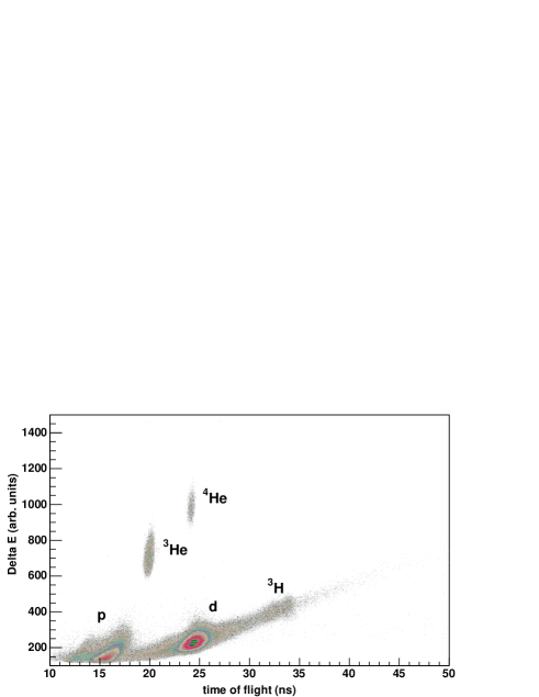
Figure 2: Energy losses in the scintillator layers versus the time of flight between them for the $d(d,X)$ reaction at 2.39 GeV/c. The islands of ³He and ⁴He are well separated from the recoil particles.

2.2 Unpolarised Angular Distribution

In the first stage of the experiment, we used an unpolarised deuteron beam incident on the target cell filled with liquid deuterium. The acceptance of the Big Karl spectrograph for $\alpha$-particles is limited, not only in momentum, but also geometrically, mainly due to the side yokes in the first dipole magnet. The consequences of this for the acceptance are shown in Fig. 3 in terms of the polar ($\theta$) and azimuthal ($\phi$) angles of the $\alpha$-particles. The regions with high acceptance that were retained in the analysis, $\pi/2-0.5\leq|\phi|\leq\pi/2+0.5$, are indicated by the solid lines. The simulated acceptance with these cuts is a smooth function ranging from 0.3 at $\cos\theta=0.4$ to 0.9 at $\cos\theta=1$.

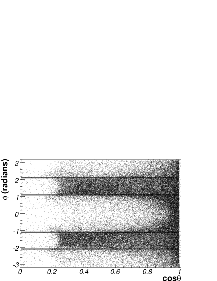
Figure 3: Measured $\alpha$-particle events after applying cuts as function of the polar angle and the cosine of the azimuthal angle in the center-of-mass frame. The regions around $\phi\approx 0$ and $\phi\approx\pm\pi$ have almost zero acceptance due to the side yoke in the first magnetic dipole.

After applying cuts, the missing mass of the detected $\alpha$-particle was evaluated and the event placed in a $\cos\theta$ bin. The resulting spectrum, summed over all angles is, shown in Fig. 4. A clear $\eta$ peak is superimposed on a background coming from multipion production. The latter was simulated by calculating the spectral form of two, three and four pion production in a phase-space model, though the shapes from two and three pion production were almost identical. The individual strengths were fitted to the experimental spectrum together with a Gaussian for the peak and the results shown in Fig. 4.

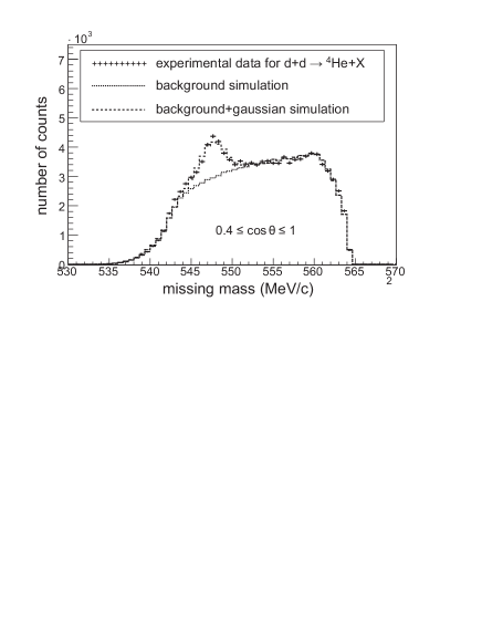
Figure 4: Missing mass distribution for the $dd\to\alpha X$ reaction in the range $0.4\leq\cos\theta\leq 1$.

An analogous analysis was applied to six bins, each of width $\Delta(\cos\theta)=0.1$. The peak areas were corrected for acceptance and converted into differential cross sections using the known luminosity. The resulting differential cross sections are shown in Fig. 5.

Figure 5: Unpolarised $dd\to\alpha\,\eta$ differential cross section. Since the entrance channel is symmetric, the data are shown in terms of $\cos^{2}\theta$. Upper panel: Data from Ref. [17] taken at $Q=7.7$ MeV. The curve is a linear fit in $\cos^{2}\theta$. Lower panel: Same as the above but for the present data at $Q=16.6$ MeV. These data are compared with a quadratic fit in $\cos^{2}\theta$.

When the incident deuterons are unpolarised, the entrance channel is symmetric and a representation of the differential cross section in terms of $\cos^{2}\theta$ is appropriate. Already at an excess energy of 7.7 MeV the ANKE collaboration found deviations from isotropy [17], with evidence of a forward dip. In contrast, the present data at $Q=16.6$ MeV show a strong peaking in the forward direction. Both sets of results are shown in Fig. 5. We defer further discussion of these distributions until section 3.

2.3 Beam Polarisation

The ion source used to generate the polarised deuteron beam is described in Ref. [22]. For this experiment, in addition to the unpolarised beam, two different combinations of vector $p_{z}$ and tensor $p_{zz}$ polarisation were used:

$$p_{z}=-1/3 p_{zz}=+1,$$ and

$$p_{z}=-1/3 p_{zz}=-1.$$ and (2.1)

The vector polarisation $p_{z}$ was measured with a low energy polarimeter placed in the injection beam line, where the deuteron energy is about 76 MeV. Using a carbon target, deuteron elastic scattering was measured with scintillating detectors. The results for the two polarisation combinations were consistent with the expectations, with $p_{z}=-0.32\pm 0.02$ and $p_{z}=-0.33\pm 0.02$. It has been shown that there is little or no loss of polarisation in the subsequent acceleration of deuterons at COSY up to the momentum of interest here [23].

The tensor polarisation of the beam was measured by scattering the accelerated deuterons from the liquid hydrogen target. The elastically scattered deuterons were then measured with Big Karl. The cross section for polarised $\vec{d}p$ elastic scattering in the backward direction can be expressed as:

$$\left(\frac{d\sigma}{d\Omega}(\theta=180\mbox{${}^{\circ}$})\right)_{\!\text{pol}}=\left(\frac{d\sigma}{d\Omega}(\theta=180\mbox{${}^{\circ}$})\right)_{\!\text{unpol}}\left[1+\mbox{${\textstyle\frac{1}{2}}$}p_{zz}A_{yy}(\theta=180\mbox{${}^{\circ}$})\right]\!.$$ (2.2)

At strictly 180^∘, there is only one analysing power, $A_{yy}=A_{xx}$, and this was measured at Saclay [24] over a broad range of deuteron momenta that covered the 2.39 GeV/c used here. The points were remeasured with smaller uncertainties by Punjabi et al. [25], and we made use of their results.

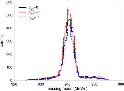
Figure 6: Missing mass spectrum for the $\vec{d}p\to pd$ reaction for the unpolarised beam (solid line) and two different tensor polarisations (dashed and dotted lines).

The outgoing deuterons were identified using the specific energy losses and time of flight. In order to eliminate background, the deuteron missing-mass spectra were analysed. An example of such a spectrum is shown in Fig. 6 for the $\vec{d}p\to dX$ process for the unpolarised beam and for both states of deuteron polarisation. In all cases there is a strong proton peak sitting on a smoothly varying background from which it was straightforward to extract the numbers of elastically scattered deuterons. The tensor polarisations summarised in Table 1 were then determined on the basis of Eq. (2.2).

Table 1: Results of the measurements of vector and tensor polarisations of the deuteron beam. The first errors are statistical and the second systematic, arising principally from the calibration polarisations [24, 25].

$p_{z}$		$p_{zz}$
nominal	measured	nominal	measured
$-1/3$	$-0.33\pm 0.02$	$-1$	$-0.87\pm 0.11\pm 0.01$
$-1/3$	$-0.32\pm 0.02$	$+1$	$+0.91\pm 0.14\pm 0.01$

2.4 Polarised Cross Section Measurement

In the subsequent experiment, we employed the vector and tensor polarised deuteron beam incident on the deuteron target to measure the analysing power in the $\vec{d}d\to\alpha\,\eta$ reaction. The following sequence of polarisation modes was used

$$\mathcal{P}_{+1}\mathcal{P}_{-1}\mathcal{P}_{+1}\mathcal{P}_{-1}\mathcal{P}_{+1}\mathcal{P}_{-1}\mathcal{P}_{+1}\mathcal{P}_{-1}\mathcal{P}_{0}\mathcal{P}_{+1}\mathcal{P}_{-1}\cdots,$$ (2.3)

where $\mathcal{P}_{i}$, $i$=$+1,-1$, is a mode with the nominal values of vector $p_{z}$ and tensor $p_{zz}$ polarisation of the beam given in Table 1. It should be noted that, in contrast to the initial experiment with the unpolarised beam, the nominally unpolarised mode $\mathcal{P}_{0}$ was prepared by employing three transitions of the source and so some small residual polarisation could not be excluded.

In the reaction frame, $\hat{z}$ is taken along the beam direction, $\hat{y}$ represents the upward normal to the COSY accelerator, and $\hat{x}=\hat{y}\times\hat{z}$. The polarised $\vec{d}d\to\alpha\,\eta$ cross section at a production angle $\theta$ can be written in Cartesian basis as

$$\underbrace{\left.\Big{(}\frac{d\sigma}{d\Omega}(\theta,\phi)\Big{)}_{\!\text{pol}}\right/\Big{(}\frac{d\sigma}{d\Omega}(\theta)\Big{)}_{\!\text{unpol}}}_{F} = \Big{[}1+\frac{3}{2}\underbrace{A_{y}(\theta)p_{z}}_{H}\cos\phi$$ (2.4)

$$+\frac{1}{4}\underbrace{p_{zz}(A_{yy}(\theta)+A_{xx}(\theta))}_{G}+\frac{1}{4}\underbrace{p_{zz}(A_{yy}(\theta)-A_{xx}(\theta))}_{J}\cos 2\phi\Big{]}.$$

The polarisation was inspected for each run by fitting the quantities $F$, $G$, $H$ and $J$ to the angular distributions on the M detector. An example of the response of the M detector to different beam polarisations is shown in Fig. 7, together with the fitted curves.

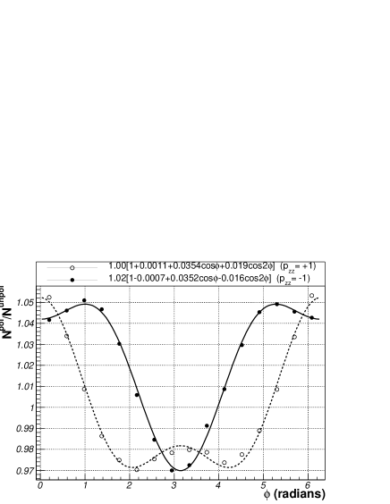
Figure 7: Ratio of the counting rate in each M detector segment, corresponding to a certain azimuthal angle $\phi$, for two different polarisations of the deuteron beam. The dashed line represents the fit result for $(p_{z},p_{zz})=(-\frac{1}{3},+1)$, while the solid line corresponds to $(p_{z},p_{zz})=(-\frac{1}{3},-1)$.

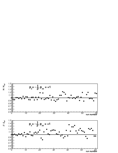
Figure 8: Comparison of the ratio of the measured parameters $H$ and $J$ to the reference values $H_{\text{ref}}$ and $J_{\text{ref}}$ for both polarisation states as functions of the run number. The $H$ parameter corresponds to the vector polarisation $p_{z}$, while $J$ is connected with the tensor beam polarisation $p_{zz}$. Left: Polarisation state with $p_{z}=-\frac{1}{3}$, $p_{zz}=+1$. Right: Polarisation state with $p_{z}=-\frac{1}{3}$, $p_{zz}=-1$.

The fitted parameters $H$ and $J$ are shown in Fig. 8 relative to the nominal values $H_{\text{ref}}$ and $J_{\text{ref}}$ for individual run numbers. The deviations from these values are less than $\pm 15\%$. Because of the smallness of these fluctuations, we retain the nominal values in the analysis.

The analysing powers could, in principle, be extracted by fitting Eq. (2.4) directly to the data. However, the present detector does not have full acceptance (see Fig. 3). Furthermore, as is seen from Eq. (2.3), the unpolarised beam in this part of the experiment had only 10% of the statistics and even here there may be some residual polarisation. We therefore developed a method to extract the analysing powers without making use of the unpolarised beam.

As indicated in Fig. 3, there are two ranges of azimuthal angle where there is almost complete acceptance, i.e.,

$$\mbox{${\textstyle\frac{1}{2}}$}(\pi-1)\leq|\phi|\leq\mbox{${\textstyle\frac{1}{2}}$}(\pi+1)\,\textrm{rad}.$$ (2.5)

For these intervals the mean value of $\cos\phi$ vanishes and that of $\cos 2\phi$ is given by

$$<\cos 2\phi>=\int_{(\pi-1)/2}^{(\pi+1)/2}\cos 2\phi\,d\phi=-0.84.$$ (2.6)

It therefore becomes clear that $A_{y}$ could not be measured with the present layout.

Since $<\cos 2\phi>$ is close to $-1$, Eq. (2.4) shows that our experiment is primarily sensitive to the values of $A_{xx}$, with only a small contamination from $A_{yy}$. We therefore neglect the contribution of $A_{xx}-A_{yy}$ to the counting rates in these intervals. In this approximation, the cross section integrated over these intervals of azimuthal angle becomes simply

$$I=\int_{(\pi-1)/2}^{(\pi+1)/2}\left(\frac{d(\theta,\phi)}{d\Omega}\right)_{\!\text{pol}}d\phi=\left(\frac{d{\sigma}}{d\Omega}(\theta)\right)_{\!\text{unpol}}\left[1+0.46\,p_{zz}A_{xx}(\theta)\right],$$ (2.7)

where the unpolarised cross section is integrated over the same $\phi$ range.

Carrying out this procedure for the two polarisation states, we find that

$$\Delta=\frac{I^{+}-I_{1}^{-}}{I^{+}+I^{-}}=\frac{0.23\,A_{xx}\left(p_{zz}^{+}-p_{zz}^{-}\right)}{1+0.23\,A_{xx}\left(p_{zz}^{+}+p_{zz}^{-}\right)}\cdot$$ (2.8)

Using the measured beam polarisations reported in Table 1, we can solve to find the value of $A_{xx}$:

$$A_{xx}=2.44\,\Delta/(1-0.02\,\Delta).$$ (2.9)

Since the unpolarised cross section drops out of Eq. (2.9), it is sufficient to count the numbers of registered $\alpha\,\eta$ events $N$ per incident beam $n$. The total numbers of beam particles for the truly unpolarised beam and the two polarisation states are given in Table 2. Uncertainties in the target thickness and in the acceptance etc. cancel.

Table 2: Integrated beam intensities for the unpolarised and polarised deuteron beams.

Nominal		Integrated beam
$p_{z}$	$p_{zz}$	intensity $n$
0	0	$(12.70\pm 0.48)\times 10^{13}$
$-\frac{1}{3}$	$+1$	$(6.98\pm 0.62)\times 10^{13}$
$-\frac{1}{3}$	$-1$	$(6.19\pm 0.51)\times 10^{13}$

As is demonstrated later, $A_{xx}$ as well as the unpolarised cross section are both even functions of $\cos\theta$ and so they are shown in Fig. 9 as functions of $\cos^{2}\theta$. The large error bars for $A_{xx}$ arise from the fluctuations in the significant background under the $\eta$ peaks. It should be noted that the analysing power $A_{xx}$ in the range just above the $\eta$ peak is found to be consistent with zero.

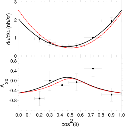
Figure 9: Upper panel: Differential cross section for the $dd\to\alpha\,\eta$ reaction. Lower panel: Analysing power $A_{xx}$. The solid curves represent a fit with four partial waves; the dotted curves with invariant amplitudes.

3 Results and Discussion

3.1 Unpolarised Cross sections

In order to deduce the total $dd\to\alpha\,\eta$ cross section, the differential data were fitted in terms of Legendre polynomials:

$$\frac{\mbox{\rm d}\sigma}{\mbox{\rm d}\Omega}=\sum_{l=0}^{\ell_{max}}a_{2l}P_{2l}(\cos\theta).$$ (3.1)

The smallest value for $2\ell_{max}$ required to describe our data was found to be four. The resulting parameters are $a_{0}=1.27\pm 0.03$ nb/sr, $a_{2}=-0.29\pm 0.06$ nb/sr, and $a_{4}=1.65\pm 0.07$ nb/sr, and the corresponding fit is shown in Fig. 5. This indicates that there must be at least $d$-wave contributions. This is to be contrasted to the lower energy ANKE results [17], where $2\ell_{max}=2$ suffices (see Fig. 5). In their case, $a_{0}=1.30\pm 0.18$ nb/sr and $a_{2}=-0.79\pm 0.19$ nb/sr which, as in our results, is negative.

The total cross section deduced from the fit is

$$\sigma=16.0\pm 0.4~{}\textrm{nb},$$ (3.2)

where uncertainties in the target thickness, incident flux, and acceptance introduce an additional systematic error of $\pm 1.6$ nb. In Fig. 10 this result is compared with existing data, which are all taken at smaller excess energies.

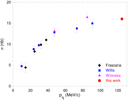
Figure 10: Excitation function for the total cross section for the $dd\to\alpha\,\eta$ reaction. The data are from Frascaria et al. [12], Willis et al. [13], and Wrońska et al. [17]. Only statistical errors are shown.

Willis et al. [13] only extracted the cross section for helicity $m=\pm 1$, which makes their result for the unpolarised total cross section model dependent. The values shown in Fig. 10 correspond to the assumption that the $p$-wave amplitude leading to the $m=0$ cross section is negligible. This is consistent with our data and we will return to the point in section 3.3, after discussing the amplitude decomposition.

3.2 Amplitudes and Observables

In order to extract the $s$-wave amplitude for $dd\to\alpha\,\eta$, we attempted to fit partial wave amplitudes

$$a_{i}=|a_{i}|\,\textrm{e}^{i\phi_{i}},$$ (3.3)

to the present data. Since the angular distributions require terms up to $\cos^{4}\theta$, we consider $s$, $p$ and (two) $d$ waves. After applying angular momentum and parity conservation, and taking into account the identical nature of the incident deuterons, it is seen that there are only four transitions, which are noted in Table 3.

Table 3: Quantum numbers corresponding to the four lowest partial waves for the $dd\to\alpha\,\eta$ reaction. Here $s_{i}$ is the total spin of the initial deuterons with orbital angular momentum $\ell_{i}$. Bose symmetry requires that $s_{i}+\ell_{i}$ be even. The total angular momentum $J$ is equal to the $\alpha\,\eta$ orbital angular momentum $\ell_{f}$.

amplitude name	$s_{i}$	$\ell_{i}$	$\ell_{f}$	wave name
$a_{0}$	1	1	0	s
$a_{1}$	2	2	1	p
$a_{2}$	1	1	2	d
$a_{3}$	1	3	2	d

Simonius has shown how to relate such amplitudes to different possible observables [26]. However, when these are fitted directly to our data it is found that only the magnitude of the $s$-wave amplitude $|a_{0}|$ is stable. In contrast, the magnitudes of the two $d$-wave amplitudes $|a_{2}|$ and $|a_{3}|$ are completely correlated. To see the origin of these effects, it is simplest to consider the relation of the partial waves to the invariant amplitudes used by Wrońska et al. [17], which we briefly summarise here.

Due to the identical nature of the incident deuterons, only three independent scalar amplitudes are necessary to describe the spin dependence of the reaction. If we let the incident deuteron cms momentum be $\vec{p}_{d}$ and that of the $\eta$ be $\vec{p}_{\eta}$, then one choice for the structure of the transition matrix $\mathcal{M}$ is

$$\mathcal{M} = A({\vec{\epsilon}}_{1}\times{\vec{\epsilon}}_{2})\cdot{\hat{p}_{d}}+B({\vec{\epsilon}}_{1}\times{\vec{\epsilon}}_{2})\cdot\left[\hat{p}_{d}\times(\hat{p}_{\eta}\times\hat{p}_{d})\right](\hat{p}_{\eta}\cdot{\hat{p}_{d}})$$ (3.4)

$$+C\left[({\vec{\epsilon}}_{1}\cdot{\hat{p}_{d}})\,{\vec{\epsilon}}_{2}\!\cdot\!(\hat{p}_{\eta}\times\hat{p}_{d})+({\vec{\epsilon}}_{2}\cdot{\hat{p}_{d}})\,{\vec{\epsilon}}_{1}\!\cdot\!(\hat{p}_{\eta}\times\hat{p}_{d})\right],$$

where the ${\vec{\epsilon}}_{i}$ are the polarisation vectors of the two deuterons.

If we retain up to $d$ waves in the final system, then $B$ and $C$ have no angular dependence while that of the amplitude $A$ can be written as

$$A(\theta)=A_{0}+A_{2}\,P_{2}(\cos\theta)\,.$$ (3.5)

The observables in a spherical basis were related to these amplitudes in Ref. [17] but they can be easily converted to the Cartesian observables used here [27]. Our experiment only yielded data on the unpolarised cross section and tensor analysing power $A_{xx}$ and these are given in terms of the invariant amplitudes by

$$\left(1-A_{xx}\right)\frac{\mbox{\rm d}\sigma}{\mbox{\rm d}\Omega} = \frac{p_{\eta}}{p_{d}}\left(|A_{0}|^{2}+2\emph{Re}(A_{0}A_{2}^{*})P_{2}(\cos\theta)+|A_{2}|^{2}\left(P_{2}(\cos\theta)\right)^{2}\right)\,,$$

(3.6)

$$\left(1+2A_{xx}\right)\frac{\mbox{\rm d}\sigma}{\mbox{\rm d}\Omega} = 2\frac{p_{\eta}}{p_{d}}\left(|B|^{2}\sin^{2}\theta\cos^{2}\theta+|C|^{2}\sin^{2}\theta\right)\,,$$ (3.7)

where the results have been expressed in terms of convenient linear combinations. From these it is seen that both the cross section and $A_{xx}$ are even functions of $\cos\theta$, a result that has already been used in our analysis and presentation. The data could therefore in principle fix the magnitudes of the amplitudes $A_{0}$, $A_{2}$, $B$, and $C$, and the interference between $A_{0}$ and $A_{2}$, while being completely insensitive to all the other phases. Furthermore, the linear combinations of Eqs. (3.6) and (3.7) show that the fitting of $|B|$ and $|C|$ is decoupled from that of $A$. The parameters resulting from fitting the data in this basis are given in Table 4, with the fit curves being shown in Fig. 9. From this it is seen that the $A$ amplitudes are dominant, with $C$ being consistent with zero within error bars. If $|B|$ also vanished, it would follow from Eq. (3.7) that $A_{xx}=-\frac{1}{2}$ for all angles. On the other hand, even the small contribution from the $B$ term changes the angular dependence of $A_{xx}$, as is evident in Fig. 9.

Table 4: Fit results of invariant amplitudes of Eqs. (3.6) and (3.7) to the present data. Since $|C|$ was found to be zero within error bars, it was put exactly to zero.

fit parameter	value
$|A_{0}|^{2}$	$\phantom{-1}6.6\pm 1.7$
$2\textit{Re}\,(A_{0}^{*}A_{2})$	$-25.0\pm 9.5$
$|A_{2}|^{2}$	$\phantom{-1}48.4\pm 14.5$
$|B|^{2}$	$\phantom{-1}9.3\pm 5.1$
$|C|^{2}$	$\phantom{-1}0$

The Wrońska et al. amplitudes can be easily expressed in terms of those of the partial waves $a_{i}$ of Table 3. Explicitly

$$\sqrt{\frac{p_{\eta}}{p_{d}}}\sqrt{4\pi}\,A_{0} = \frac{1}{3\sqrt{2}}\,a_{0}\,,$$

$$\sqrt{\frac{p_{\eta}}{p_{d}}}\sqrt{4\pi}\,A_{2} = \sqrt{5}\left[\frac{1}{\sqrt{14}}\,a_{3}-\frac{1}{3}\,a_{2}\right],$$

$$\sqrt{\frac{p_{\eta}}{p_{d}}}\sqrt{4\pi}\,B = \frac{\sqrt{5}}{2}\left[a_{2}+\sqrt{\frac{2}{7}}\,a_{3}\right],$$

$$\sqrt{\frac{p_{\eta}}{p_{d}}}\sqrt{4\pi}\,C = \frac{1}{2}\sqrt{\frac{3}{5}}\,a_{1}\,.$$ (3.8)

From the above discussion, it is seen that if $\ell_{\eta}=4$ waves are neglected, then the data might determine the absolute magnitudes of the $\ell_{\eta}=0$ and $\ell_{\eta}=1$ amplitude, viz. $|a_{0}|$ and $|a_{1}|$. On the other hand, only two linear combinations of the $d$-wave amplitudes $|a_{2}+2a_{3}/\sqrt{14}|^{2}$ and $|a_{2}-3a_{3}/\sqrt{14}|^{2}$ could fixed by the data. Thus the differential cross section and tensor analysing power $A_{xx}$ are together only sensitive to $7|a_{2}|^{2}+3|a_{3}|^{2}$ rather than the individual magnitudes. This accounts for the complete correlation found in the direct fitting of the partial wave amplitudes to the data.

3.3 The s-Wave Amplitude

We have seen that, provided $g$-waves are neglected, the present data allow us to extract the magnitude of the $s$-wave amplitude $|a_{0}|$. From this we obtain a spin-averaged square of the $s$-wave amplitude, $|f_{s}|^{2}$ through

$$\frac{\mbox{\rm d}\sigma_{s}}{\mbox{\rm d}\Omega}=\frac{p_{\eta}}{p_{d}}|f_{s}|^{2}=\frac{2p_{\eta}}{3p_{d}}|A_{0}|^{2}=\frac{1}{27}\frac{1}{4\pi}|a_{0}|^{2},.$$ (3.9)

Using the value given in Table 4, we find that $|f_{s}|^{2}=4.4\pm 1.1$ nb/sr.

Close to threshold, where $s$-waves dominate, $|f_{s}|^{2}$ can be extracted from the total cross section $\sigma$ via

$$|f_{s}|^{2}=\frac{p_{d}}{p_{\eta}}\frac{\sigma}{4\pi}\,,$$ (3.10)

since the contribution from $s$-$d$ interference drops out.

Equation (3.10) has been used by Willis et al. [13] to extract $|f_{s}|$ but there are two important considerations here. Our data show that the $B$ and $C$ amplitudes play only a minor role in the observables and this is likely to be even more true at lower energies. Hence to a good approximation the $m=0$ cross section can be neglected and the total cross section should be two thirds of their $m=\pm 1$ value. This result has already been used when plotting the data in Fig. 5.

Furthermore, although the SPESIII detector had complete acceptance for the $\alpha$ particles from $\eta$ production, the full polar angle could not be reconstructed and the authors assumed isotropic distributions [13]. While this is a good approximation close to threshold, it is not valid at their two highest energies, as is evident when comparing with the data of Ref. [17]. There will therefore be $d$-wave contributions which must be subtracted in Eq. (3.9) before extracting $|f_{s}|^{2}$. To do this, we assume that the $d$-wave amplitudes $A_{2}$ and $B$ vary with a threshold factor of $p_{\eta}^{2}$, where the normalisation is fixed by our results given in Table 4.

This procedure results $|f_{s}|^{2}=13.8\pm 1.2$ nb/sr at $p_{\eta}=73$ MeV/$c$ and $10.6\pm 1.3$ nb/sr at $p_{\eta}=91$ MeV/$c$ for the Willis data [13] and $14.3\pm 2.4$ nb/sr for the Wrońska measurement at 86 MeV/c [17]. All the values of $|f_{s}|^{2}$ are then shown in Fig. 11.

Willis et al. [13] did a combined optical-model fit to all the near-threshold $pd\to\eta^{\,3}$He and $dd\to\eta^{\,4}$He data as discussed in the introduction, assuming that only s-wave production occurred, and found a value of the $\eta\,\alpha$ scattering length of $a=(-2.2+i1.1)$ fm. Given the extended $dd\to\eta^{\,4}$He data set now available, we have attempted a direct fit in the scattering-length approximation

$$|f_{s}|^{2}=\frac{|f_{B}|^{2}}{1+p_{\eta}^{2}(a_{r}^{2}+a_{i}^{2})+2p_{\eta}a_{i}}$$ (3.11)

The best fit shown in Fig. 11 is obtained for $|a_{r}|=3.1\pm 0.5$ fm, $a_{i}=0\pm 0.5$ fm and $f_{B}^{2}=34\pm 1$ nb/sr, corresponding to a quasi-bound or virtual state with $|Q_{0}|\approx 4$ MeV. These above-threshold data are, of course, insensitive to the sign of $a_{r}$ so that they could never tell whether the system is quasi-bound or virtual. The argument given in Ref. [13] is that, since $\eta^{\,4}$He is more likely to be bound than $\eta^{\,3}$He, the fact that $|Q_{0}|$ is smaller for $\eta^{\,3}$He [10, 14, 15], suggests that $\eta^{\,4}$He is indeed quasi-bound.

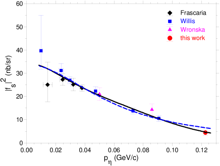
Figure 11: The world data for spin-averaged square of the magnitude the $s$-wave amplitude for $dd\to\eta^{\,4}$He as a function of the $\eta$ cm momentum. The dashed curve shows the best fit Eq. (3.11) with parameters given in the text. The solid curve is a fit with Eq. (3.12).

To try to explore the systematic uncertainties, one can include also an effective range term $r$, as has been done for the near-threshold $dp\to\eta^{\,3}$He data [14] and fit

$$f_{s}=\frac{f_{B}}{1-ip_{\eta}a+\frac{1}{2}arp_{\eta}^{2}}.$$ (3.12)

However, due to the strong coupling between the fit parameters, the error bars become exceedingly large, $a_{r}=6.2\pm 1.9$ fm and $a_{i}=0.0.001\pm 6.5$ fm. This fit is also shown in Fig. 11. The large errors here do not allow a decisive answer on the position of the $\eta\,\alpha$ pole.

4 Summary

We have measured the differential cross section and tensor analysing power $A_{xx}$ of the $dd\to\alpha\,\eta$ reaction at an excess energy of 16.6 MeV. The recoiling $\alpha$-particles were measured in a magnetic spectrograph and the $\eta$ mesons identified through a missing-mass technique. The biggest uncertainty in the method arises from the large background coming from multipion production. Despite this, an angular distribution and a total cross section could be given.

The angular distribution of the analysing power $A_{xx}$ was measured with a tensor polarised beam. Since this observable required measurements with two different spin modes, the uncertainty due to the background subtraction is even larger. Nevertheless, the values thus obtained showed that $p$-wave amplitude was very small so that deviations from isotropy must come primarily from $s$–$d$ interference [13, 17].

Combining these results with the unpolarised cross section data allowed the spin-averaged square of the $s$-wave amplitude $|f_{s}|^{2}$ to be extracted with reasonable error bars. Assuming that the $d$-wave production cross section varied like $Q^{2}$, values of $|f_{s}|^{2}$ were also deduced from earlier measurements such that there are now 13 values for $Q\leq 16.6$ MeV. Fitting the momentum dependence in the scattering length approximation [7, 8] gives $|a_{r}|=3.1\pm 0.5$ fm and $a_{i}=0.0\pm 0.5$ fm. This suggests that there is a singularity in the complex plane close to threshold but its position is far from clear and the uncertainty grows if a fit is attempted with an effective range as well as a scattering length. Further data are clearly needed!

References

- [1] Q. Haider, L.C. Liu, Phys. Lett. B 172 (1986) 257.
- [2] R.S. Bhalerao, L.C. Liu, Phys. Rev. Lett. 54 (1985) 865.
- [3] R.S. Hayano, S. Hirenzaki, A. Gillitzer, Eur. Phys. J. A 6 (1999) 99.
- [4] C. Garcia-Recio, T. Inoue, J. Nieves, E. Oset, Phys. Lett. B 550 (2002) 47.
- [5] Q. Haider, L.C. Liu, Phys. Rev. C 66 (2002) 045208.
- [6] T. Ueda, Phys. Rev. Lett. 66 (1991) 297.
- [7] K.M. Watson, Phys. Rev. 88 (1952) 1163.
- [8] A.B. Migdal, JETP 1 (1955) 2.
- [9] J. Berger. et al., Phys. Rev. Lett. 61 (1988) 919
- [10] B. Mayer, et al., Phys. Rev. C 53 (1996) 2068.
- [11] C. Wilkin, Phys. Rev. C 47 (1993) R938.
- [12] R. Frascaria, et al., Phys. Rev. C 50 (1994) R537.
- [13] N. Willis, et al., Phys. Lett. B 406 (1997) 14.
- [14] T. Mersmann, et al., Phys. Rev. Lett. 98 (2007) 242301.
- [15] J. Smyrski, et al., Phys. Lett. B 649 (2007) 258.
- [16] C. Wilkin, et al., Phys. Lett. B 654 (2007) 92.
- [17] A. Wrońska, et al., Eur. Phys. J. A 26 (2005) 421.
- [18] M. Drochner, et al., Nucl. Phys. A 643 (1998) 55.
- [19] J. Bojowald, et al., Nucl. Instrum. Methods A 487 (2002) 314.
- [20] C. Amsler, et al., Phys. Lett. B 667 (2008) 1.
- [21] V. Jaeckle, et al., Nucl. Instrum. Methods A 349 (1994) 15.
- [22] O. Felden, R. Gebel, P. von Rossen, Nucl. Instrum. Methods A 536 (2005) 278.
- [23] D. Chiladze, et al., Phys. Rev. STAB 9 (2006) 050101.
- [24] J. Arvieux, et al., Phys. Rev. Lett. 50 (1983) 19.
- [25] V. Punjabi et al., Phys. Lett. B 350 (1995) 178.
- [26] M. Simonius, Lecture Notes in Physics, 30 (1973) 38.
- [27] G.C. Ohlsen, Rep. Prog. Phys. 35 (1972) 717.