Weak-field Hall effect and static polarizability of Bloch electrons

Abstract

A theory of the weak field Hall effect of Bloch electrons based on the analysis of the forces acting on electrons is presented. It is argued that the electric current is composed of two contributions, that driven by the electric field along current flow and the non-dissipative contribution originated in demagnetization currents. The Hall resistance as a function of the electron concentration for the tight-binding model of a crystal with square lattice and body-centered cubic lattice is described in detail. For comparison the effect of strong magnetic fields is also discussed.

I Introduction

Standard linear response theories for electronic transport are formulated to obtain the conductivity tensor. Some models for scattering are needed to get a finite response. The most popular approximation is the elastic scattering approach, despite the fact that it cannot compensate the electron acceleration due to the applied electric field. It can only be compensated by a momentum dissipation, which can ensure that the total force acting on electrons vanishes in the steady state. Another possibility is to analyze forces acting on electrons in the transport regime. The condition of the vanishing total force is the basic physical condition for the steady state. The application of the linear response approach, limiting the problem to the case of small deviation from the equilibrium, gives the transport coefficients satisfying the steady state condition. This idea will be used to determine the Hall resistance of a system of Bloch spinless electrons in the case of a weak magnetic field. For the sake of simplicity we limit our consideration to isotropic systems where the energy spectrum is represented by a single electron band. It can be expected that in this case the Hall resistance will not depend on the dissipation explicitly, which can simplify the analysis substantially.

The Hall resistance is standardly measured on the so-called Hall bar samples, having the form of a long strip. Far from the contacts the current density is parallel to the strip edges, say along $\hat{x}$-direction. If the magnetic field is applied perpendicularly to the strip surface, along $\hat{z}$-direction, the current induced Lorentz force is shifting the electron charge distribution. As the result there appears a non-equilibrium charge distribution giving rise the Hall voltage. The steady state requires the compensation of the Lorentz force by the gradient force. For isotropic systems this condition can be written in the following form

$$\frac{B}{c}\,j_{x}\,=\,-\,\left\langle\frac{dV(\vec{r})}{dy}\right\rangle\,\equiv\,-\,\frac{dP(\mu)}{dy}\;,$$ (1)

where $j_{x}$ is the current density, $V(\vec{r})$ denotes the background potential including that given by the electric field along $\hat{y}$ direction, ${\cal{E}}_{y}$, and $\mu$ stands for electro-chemical potential. Angular brackets represent quantum-mechanical and statistical average. The internal pressure $P(\mu)$ represents the force of the electron ensemble acting on the external system per unit area. Linear response approximation with respect to the electro-chemical potential gradient leads to the following expression for the Hall resistance

$$R_{H}\,\equiv\,\frac{U_{H}}{J}\,=\,-\,\frac{B}{ec\left(\frac{\partial P(\mu)}{\partial\mu}\right)_{B}d}\;,$$ (2)

where $J$ is the applied current through the strip of thickness $d$ and $U_{H}$ denotes the voltage drop between strip edges.

The gradient force and consequently the pressure are quantities which are generally dependent on the magnetic field strength $B$. In the weak field limit the Hall resistance can be supposed a linear function of $B$ which implies that the $B$-dependent internal pressure can be replaced by its zero field limit. For a free electron gas (resp. hole gas) it can be identified with the so-called statistical pressure, and its derivative with respect to $\mu$ is simply equal to the electron concentration $N(\mu)$ (resp. to the negative value of the hole concentration) Landau . Considering a single electron band the Hall resistance for chemical potentials in the vicinity of band edges is thus quite well understood. Since it has opposite signs at opposite band edges it should vanish at the band center. To our knowledge, the only published work in which the transition between electron to hole like character of the Hall resistance has been described was based on the application of the Kubo formula for the special case of substitutional alloys Velicky . However, no procedure based on force analysis has been presented. A previous publication Streda_wf made by one of us was unfortunately based on incorrect application of the quasi-classical approach as will be specified later.

In crystalline solids the equilibrium electron charge distribution cannot be assumed as uniform. It is periodic in real space, having translation symmetry given by the lattice periodicity. Non-zero current density gives rise to the Lorentz force inducing a shift of the mass-center positions. This shift has to be compensated by the gradient force trying to return it back into the equilibrium distribution. The results generally depend on the experimental set up, particularly the way how the non-zero current density is induced.

In the regime we will call as fully dissipative, the current is supposed to be exclusively given by the electric field ${\cal{E}}_{x}$ along strip axis. In other words, if ${\cal{E}}_{x}\rightarrow 0$ the current vanishes. This assumption requires that dissipation take place within the strip, i.e. that the system can be viewed as a macroscopic system. It can be expected that this fully dissipative regime represents the conditions of the standardly measured Hall resistance in the weak field limit for which it can be assumed that the effect of the magnetic field to the energy spectrum is negligible.

The opposite limiting case is the purely non-dissipative regime for which the current density is exclusively determined by the electric field ${\cal{E}}_{y}$ across the strip, while ${\cal{E}}_{x}=0$. Such a situation is observed whenever the Fermi energy is located within the conduction gaps, i.e. when the magnetic field is strong enough to induce energy gaps giving rise to a Hofstadter type spectrum Hofstadter . It has already been shown that in such a quantum Hall regime the induced Hall current is closely related to the static electron polarizability Streda_07 ; Streda_08 . The non-dissipative regime, for which the Hall current is exclusively determined by the orbital magnetization, can be in principle induced even if the Fermi energy is located within the energy band. This regime, in the considered weak field limit, will also be analyzed, although the resulting effect is expected to be small, of the order $B^{2}$.

The main attention will be devoted to the fully dissipative regime. Vanishing of the total shift of the mass-center position will be taken as the steady state condition. It will be shown that it is equivalent to the condition of vanishing acceleration along the direction perpendicular to both the current flow and the magnetic field direction. For the sake of simplicity the outlined idea will be described in detail for a two-dimensional electron system since the extension to three-dimensional systems is straightforward. We will limit our consideration to the case of a single band given by a square array of tight-binding atomic states. This model will be described in Section II. The following Section will be devoted to the determination of the mass-center shifts within the quasi-classical approach. The obtained results we will be used to determine properties of macroscopic systems at zero temperature. In Section IV the magnetic moment due to the motion of mass-center positions will be analyzed and its main features compared with those well known for the case of a strong magnetic field. In Section V explicit expressions for the Hall resistance and the statistical pressure will be derived. As an example of three-dimensional system the properties of a body-centered cubic lattice of tight-binding states will be presented. The Section VI will be devoted to the non-dissipative regime, which is closely related to the effect of the magnetic field on the static electron polarizability. It will be shown that the polarizability of open systems is modified by the Lorentz force giving rise to a non-dissipative Hall current exclusively determined by demagnetization currents. In the Section VII it will be argued that in standard Hall bar measurement the current flow is composed of two contributions, that induced by the electric field along the current flow and that originated in demagnetization currents. The resulting general formula for the Hall resistance will be presented and its properties briefly discussed. The paper will be closed with short summary.

II Zero-field energy spectra

Tight-binding model is the standard approach to model band structure of crystals. If periodic boundary conditions are applied eigenfunctions are of Bloch form, characterized by the wave vector $\vec{k}$. Assuming square lattice and non-zero overlaps between atomic functions located at the nearest neighbor atomic sites only, the single-band energy spectrum is

$$E^{(0)}(\vec{k})=-2V_{0}\,\left[\cos(k_{1}a)+\cos(k_{2}a)\right]\;,$$ (3)

where $a$ and $V_{0}$ denote lattice constant and overlap integral, respectively. The components of the wave vector $\vec{k}$ along the main crystallographic axes, (1,0) and (0,1), are $k_{1}$ and $k_{2}$, respectively. The position of the band center given by the energy of the atomic orbitals, which can be represented by a confining frequency $\Omega_{0}$, has been chosen as the origin of the energy scale.

The wave numbers $k_{1}$ and $k_{2}$ are not the only choice to characterize the eigenstates. The square lattice has a translation symmetry along (1,$\pm$ 1) crystallographic directions as well. Choosing components of the wave vector along these directions to characterize Bloch states, $\kappa\equiv(k_{1}+k_{2})/\sqrt{2}$ and $\beta\equiv(k_{1}-k_{2})/\sqrt{2}$, eigenenergies become

$$E^{(0)}_{\beta}(\kappa)\,=\,-4V_{0}\,\cos\left(\kappa\tilde{a}\right)\,\cos\left(\beta\tilde{a}\right)\;,$$ (4)

where $\tilde{a}=a/\sqrt{2}$. Energy dispersions are shown in Fig. 1. In the inset the used elementary cell in the $(\kappa,\beta)$ space, which has been chosen as $\tilde{a}\beta\in[-\pi/2,\pi/2]$ and $\tilde{a}\kappa\in[-\pi,\pi]$, is shown. Since the second derivatives of the energy with respect of $\beta$ as well as $\kappa$ are equivalent, these states represent quasiparticles having isotropic effective mass

$$\frac{1}{m^{\ast}_{\beta}(\kappa)}=-\frac{a^{2}E_{\beta}^{(0)}(\kappa)}{2\hbar^{2}}=\frac{\cos\left(\beta\tilde{a}\right)}{m^{\ast}_{\rm edge}}\,\cos\left(\kappa\tilde{a}\right)\,\;,$$ (5)

where $m^{\ast}_{\rm edge}$ denotes the absolute value of the effective mass at band edges, $m^{\ast}_{\rm edge}=\hbar^{2}/(2V_{0}a^{2})$. All quasiparticles of the same energy have the same effective mass. This property simplifies the quasi-classical approach which will be described in the following Section. At negative energies, $\kappa\tilde{a}\,\epsilon\,(-\pi/2,\pi/2)$, quasiparticles have electron-like character with positive effective mass while at positive energies, $\kappa\tilde{a}\,\epsilon\,\pm(-\pi,-\pi/2)$, quasiparticles have hole-like character with negative effective mass.

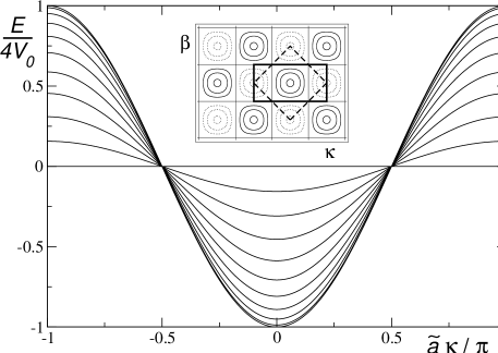
Figure 1: Energy dispersions of the tight-binding model for several fixed values of $\beta\in[-\pi/(2\tilde{a}),\pi/(2\tilde{a})]$. The same dispersions are obtained for fixed values of $\kappa$. In the inset equi-energy contours are shown in the $\kappa,\beta$ space. Full and dotted lines correspond to states having electron or hole like character, respectively. The dashed line shows the boundary of the standard first Brillouin zone, while the bold line shows the elementary cell we are using.

Electronic transport is studied on samples having the form of a long strip with a finite width $w$. It is thus natural to assume periodic boundary conditions along the direction given by the strip axis only. The eigenfuctions thus have Bloch-like character along strip axis, while along perpendicular direction they are of limited range. If the strip width can be counted as macroscopic, eigenenergies are practically untouched by the change of the boundary conditions. For isotropic systems, like the considered square lattice, the measured transport coefficient are independent of the strip orientation. We can thus choose the strip axis to be parallel with the (1,1) crystallographic direction without loss of generality. In this case the eigenfunctions can be approximated by a linear combination of Bloch states $|\beta,\kappa\rangle$ and $|-\beta,\kappa\rangle$. The index $\beta$ can be then viewed as the branch index representing bound modes across the strip. In such the case the only nonzero component of the velocity expectation value is along strip axis

$$v^{(0)}_{\beta}(\kappa)\,=\,\frac{2\sqrt{2}V_{0}a}{\hbar}\,\sin(\kappa\tilde{a})\,\cos(\beta\tilde{a})\;.$$ (6)

III Effective Hamiltonian : quasi-classical approximation

In the spirit of the preceding Section we consider a strip opened along the $\hat{x}$ direction which coincides with (1,1) crystallographic direction of the considered square lattice. The applied magnetic field along the $\hat{z}$ direction and the electric field across strip, i.e. along the $\hat{y}$ direction, ${\cal{E}}_{y}$, give rise to the Lorentz force and electric force, respectively. To preserve the Bloch character of the wavefunctions along the $\hat{x}$ direction the Landau gauge for vector potential is used, $\vec{A}\equiv(-By,0,0)$. We include it into the Hamiltonian by using the so-called Peierls substitution Peierls ; Luttinger . Since the effective mass of quasiparticles is isotropic we can use the following effective Hamiltonian

$$H_{\rm eff}^{(\beta,\kappa)}(y)\,=\,\frac{p_{y}^{2}}{2m_{\beta}^{\ast}(\kappa)}\,+\,E_{\beta}^{(0)}\left(\kappa-l_{B}^{-2}y\right)\,+$$

$$+\,e{\cal{E}}_{y}y+\frac{1}{2}\,m_{\beta}^{\ast}(\kappa)\,\Omega_{0}^{2}y^{2}\,-\frac{\pm 1}{2}\,\hbar\Omega_{0}\;,$$ (7)

where the $\pm 1$ corresponds to the sign of the effective mass $m^{*}_{\beta}(\kappa)$, and $l_{B}$ denotes the magnetic length, which is related to the cyclotron frequency $\omega_{c}$ as

$$l_{B}^{2}\,\equiv\,\frac{\hbar c}{eB}\,=\,\frac{\hbar}{m_{0}\omega_{c}}\;.$$ (8)

The last term of the effective Hamiltonian $\pm\hbar\Omega_{0}/2$ appears to preserve the origin of the energy scale given by the oscillator energy $\hbar\Omega_{0}$. The energy operator $E_{\beta}^{(0)}(\kappa-l_{B}^{-2}y)$ is defined by its Taylor expansion in $\kappa$, and in the considered case of the weak field limit only terms up to the second order are preserved. The effective Hamiltonian then becomes simply the one of an effective harmonic oscillator

$$H_{\rm eff}^{(\beta,\kappa)}(y)=\frac{p_{y}^{2}}{2m_{\beta}^{\ast}(\kappa)}+\frac{m_{\beta}^{\ast}(\kappa)}{2}\,\tilde{\Omega}^{2}\left[y-Y_{\beta}(\kappa)\right]^{2}+$$

$$-\frac{1}{2}\,m_{\beta}^{\ast}(\kappa)\,\tilde{\Omega}^{2}\left[Y_{\beta}(\kappa)\right]^{2}\,+\,E_{\beta}^{(0)}(\kappa)\,-\,\frac{\pm 1}{2}\,\hbar\Omega_{0}\,,\;$$ (9)

where $Y_{\beta}(\kappa)$ denotes the expectation value of the mass-center position

$$Y_{\beta}(\kappa)=\frac{m_{0}\omega_{c}v_{\beta}^{(0)}(\kappa)-e{\cal{E}}_{y}}{m_{\beta}^{\ast}(\kappa)\tilde{\Omega}^{2}}\;,$$ (10)

and

$$\tilde{\Omega}^{2}\,\equiv\,\Omega_{0}^{2}+\left(\frac{m_{0}}{m^{\ast}_{\beta}(\kappa)}\right)^{2}\omega_{c}^{2}\;.$$ (11)

Resulting eigenenergies are

$$E_{\beta}(\kappa)=\pm\hbar\frac{\tilde{\Omega}-\Omega_{0}}{2}+E^{(0)}_{\beta}(\kappa)-\frac{m_{\beta}^{\ast}(\kappa)}{2}\,\tilde{\Omega}^{2}\,\left[Y_{\beta}(\kappa)\right]^{2}.$$ (12)

The expectation of the velocity along the strip axis has the following expression

$$v_{\beta}(\kappa)\,=\,v^{(0)}_{\beta}(\kappa)\,-\,\frac{m_{0}}{m_{\beta}^{\ast}(\kappa)}\,\omega_{c}\,Y_{\beta}(\kappa)\;,$$ (13)

which coincides with the well known result for magnetic field corrections to the velocity Kubo .

The corrections to the energy, as well as to the velocity, due to the presence of magnetic and electric fields are proportional to square of these fields or their product. In the weak field limit, $B\rightarrow 0$ and ${\cal{E}}_{y}\rightarrow 0$, these corrections can thus be neglected and the only effect that will be considered is the change of the quasiparticle dynamics, represented in our description by the change of their mass-center positions. This approach which will be used in the following treatment is in accord with the standard quasi-classical view. To support this let us consider the product $\Omega_{0}^{2}Y_{\beta}(\kappa)$ representing the quasiparticle acceleration $a_{y}(\beta,\kappa)$ along $\hat{y}$ direction. From Eq. (10) we get

$$a_{y}(\beta,\kappa)\,=\,\frac{m_{0}\omega_{c}v_{\beta}^{(0)}(\kappa)-e{\cal{E}}_{y}}{m_{\beta}^{\ast}(\kappa)}\;.$$ (14)

This relation leads to the conclusion that in crystals the acceleration of quasiparticles is modified by their effective mass which is in agreement with the quasi-classical approach presented e.g. in Landau-Lifshitz textbook Landau . Note that the quasiparticle acceleration along the $\hat{y}$ direction induced by the electric field ${\cal{E}}_{y}$ originates in their transfer between branches $\beta$.

The presented quasi-classical approach neglects the interference effects induced by the magnetic field which are responsible for modification of the energy spectrum. A number of energy gaps are created and the energy structure is of the Hofstadter type Hofstadter . In weak field limit, the gaps in the energy spectrum becomes extremely small, and it can be expected that theses interferences will be destroyed by dissipative processes always present at finite temperatures. For this reason the presented quasi-classical approach is acceptable.

IV Magnetic moment of Fermi electrons

The applied magnetic field along the $\hat{z}$ direction gives rise to the magnetic moment $M_{z}(\mu)$. Generally $M_{z}(\mu)$ can be divided into two contributions: $M_{z}^{(i)}(\mu)$ given by the internal momentum of quasiparticles and $M_{z}^{(a)}(\mu)$ due to the motion of their mass-centers. The second contribution can be viewed as the macroscopic one since the trajectories of the mass-center positions are extended along the $\hat{x}$ direction. It can easily be determined within the quasi-classical approximation presented in the preceding Section. Its expectation value reads

$$M_{z}^{(a)}(\beta,\kappa)\,=\,\frac{e}{c}\,v_{\beta}^{(0)}(\kappa)\,Y_{\beta}^{(B)}(\kappa)\;,$$ (15)

where in accord with Eq. (10)

$$Y_{\beta}^{(B)}(\kappa)\,=\,\frac{m_{0}\omega_{c}v_{\beta}^{(0)}(\kappa)}{m_{\beta}^{\ast}(\kappa)\Omega_{0}^{2}}\;.$$ (16)

Defining the dimensionless quantity $\tilde{\sigma}(\mu)$ as

$$\tilde{\sigma}(\mu)\equiv\frac{2\pi}{w}\sum_{\beta,\kappa}f_{0}\left(E_{\beta}^{(0)}(\kappa)-\mu\right)\frac{dY_{\beta}^{(B)}(\kappa)}{d\kappa}\;,$$ (17)

where $w$ is the strip width, the Fermi electron contribution per unit area reads

$$\left(\frac{\partial M_{z}^{(a)}(\mu)}{\partial\mu}\right)_{B}\,=\,\frac{e}{hc}\,\tilde{\sigma}(\mu)\;.$$ (18)

The relation between $M_{z}^{(a)}(\mu)$ and $\tilde{\sigma}(\mu)$ defined by Eq. (17) is quite general and for the case of quantizing magnetic fields and weak periodic modulation has already been discussed in detail, where $\tilde{\sigma}(\mu)$ was called the effective topological number Streda_08 ; Streda_07 .

In the weak field limit, for the square lattice, performing the $\kappa$ integration in Eq. (17) gives

$$\tilde{\sigma}(\mu)=\frac{1}{w}\sum_{\beta}2Y^{(B)}_{\beta}(\kappa^{\beta}_{F})$$ (19)

where $\kappa^{\beta}_{F}$ if the positive value of $\kappa$ on the Fermi surface for a given $\beta$. Using $1/m^{*}_{\beta}(\kappa^{\beta}_{F})=-\mu/(4V_{0}m^{*}_{edge})$, we finally get

$$\tilde{\sigma}(\mu)\,=\,-\,\frac{m_{0}}{m^{\ast}_{\rm edge}}\,\frac{\omega_{c}}{\Omega_{0}}\,\frac{\mu}{\hbar\Omega_{0}}\,\pi a^{2}\,N_{\rm eff}(\mu)\;,$$ (20)

where

$$N_{\rm eff}(\mu)\,\equiv\,\frac{2}{\pi^{2}a^{2}}\int_{0}^{\phi_{0}}\sqrt{\cos^{2}\phi-\cos^{2}\phi_{0}}\,d\phi\;,$$

$$\phi_{0}={\rm arccos}(|\mu|/4V_{0})\;.$$ (21)

At the band edges the effective quasiparticle concentration $N_{\rm eff}(\mu)$ approaches the electron or hole concentration $m^{*}_{edge}/(2\pi\hbar^{2})\Delta E$ with $\Delta E=\mu+4V_{0}$ for electrons and $\Delta E=4V_{0}-\mu$ for holes. Energy dependence of $\tilde{\sigma}(\mu)$ and $N_{\rm eff}(\mu)$ are shown in Fig. 2.

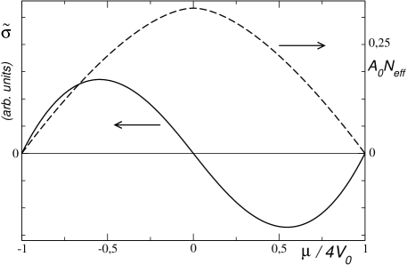
Figure 2: Energy dependence of the effective topological number $\tilde{\sigma}(\mu)$, full line, and the effective quasiparticle number in a unit cell $A_{0}N_{\rm eff}(\mu)$, dashed line.

At negative energies, $\mu<0$, for which quasiparticles have electron-like character, the Fermi contribution to $M_{z}^{(a)}(\mu)$ given by Eq. (18) is positive, i.e. it represents paramagnetic contribution to the total magnetic moment. It is often interpreted as a contribution given by electrons skipping along sample edges, which fully compensates the diamagnetic moment of electrons in the classical limit. In the presented model it has been equally splited over the local strips of tight-binding atomic orbitals. At positive energies the contribution of Fermi particles to $M_{z}^{(a)}(\mu)$ has opposite sign revealing electron-hole symmetry. At the band center it vanishes, $\tilde{\sigma}(\mu)\rightarrow 0$. This is the consequence of the electron-hole symmetry and this feature persists even in the case of strong magnetic fields affecting energy spectra substantially Streda_08 . Similarly, when the energy band is fully occupied, $\tilde{\sigma}(\mu)\rightarrow 0$ in the weak field limit, as well as in the case of quantizing magnetic fields.

V Hall resistance: fully dissipative regime

V.1 Square lattice

The electric field along the strip axis, ${\cal{E}}_{x}$, accelerates electrons along the $\hat{x}$ direction. This effect can be modelled by including the time dependent vector potential $\vec{A}(t)\equiv(-e{\cal{E}}_{x}t,0,0)$ into the Hamiltonian. For small values of the electric field and short times the linear response gives the following change of the quasiparticle velocity

$$v_{\beta}^{(0)}(\kappa-e{\cal{E}}_{x}t/\hbar)\,\approx\,v_{\beta}^{(0)}(\kappa)\,-\,\frac{dv_{\beta}^{(0)}(\kappa)}{d\kappa}\,\frac{e{\cal{E}}_{x}t}{\hbar}\;,$$ (22)

where corrections to the velocity proportional to $B^{2}$, Eq. (13), have been neglected. Summation over occupied states gives the current density along $\hat{x}$ direction

$$j_{x}(\mu)\,=\,\frac{eN_{\rm eff}(\mu)}{m^{\ast}_{\rm edge}}\,e{\cal{E}}_{x}t\;.$$ (23)

Change of the velocities gives rise to the shift of mass-center positions of quasiparticles, Eq. (16). Summation over occupied states leads to the following expression for mass-center shift $\langle\Delta Y^{(B)}(\mu)\rangle$ of the electron density within the unit cell area

$$\frac{\langle\Delta Y^{(B)}(\mu)\rangle}{A_{0}}\,=\,-\frac{\tilde{\sigma}(\mu)}{2\pi}\,\frac{e{\cal{E}}_{x}t}{\hbar}\,=\,\frac{Bj_{x}}{c\,m^{\ast}_{\rm edge}\Omega_{0}^{2}}\,\frac{\mu}{4V_{0}}\,.$$ (24)

Evidently this time dependent shift is induced by the Lorentz force.

The shift of the mass-center position is closely related to the shift of the electron charge distribution with respect of the periodic positive background charge. It gives rise to the Coulomb energy. For the system is thus energetically more acceptable to induce electric field along $\hat{y}$ direction, ${\cal{E}}_{y}$, which would be able to minimize the Coulomb energy, i.e. to force shifted electron charge distribution towards its equilibrium one. In the presented model this force is represented by the confining potential of the strength given by the frequency $\Omega_{0}$. Standard condition to estimate the induced field ${\cal{E}}_{y}$ is the condition of vanishing acceleration given by Eq. (14). It coincides with the condition of vanishing average shift of mass center positions defined by Eq. (10). Summation over occupied states gives

$$\frac{Bj_{x}}{cm^{\ast}_{\rm edge}}\frac{\mu}{4V_{0}}\,-\,e{\cal{E}}_{y}\frac{N_{\rm eff}(\mu)}{m^{\ast}_{\rm edge}}\,=\,0\,.$$ (25)

For the Hall resistance we get

$$R_{H}(\mu)\,\equiv\,\frac{{\cal{E}}_{y}}{j_{x}}\,=\,\frac{B}{ecN_{\rm eff}(\mu)\,\frac{4V_{0}}{\mu}}\,.$$ (26)

The energy dependence of the Hall resistance is shown on Fig. 3. It shows clearly the electron hole symmetry. At band edges, $\mu\rightarrow\pm 4V_{0}$, $N_{\rm eff}(\mu)$ approaches quasiparticle concentration and the classical result for the Hall resistance is recovered.

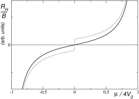
Figure 3: Energy dependence of the Hall resistance for a two-dimensional square lattice. Dotted line represents the classical resistance for free carriers, i.e. the quantity $4V_{0}N_{\rm eff}(\mu)/\mu$ is replaced by the negative value of the electron concentration ($\mu<0$) or by the hole concentration ($\mu>0$).

To approach a steady state an energy dissipation is necessary to eliminate the acceleration induced by ${\cal{E}}_{x}$. The standard way is to assume exponential decay of momentum characterized by the relaxation time $\tau$. In other words the time entering expression for the current density, Eq. (23), has to be replaced by $\tau$, which is in general a $\mu$ dependent quantity. Although the Hall resistance does not explicitly depends on the momentum relaxation it is essential for application of the linear response with respect of ${\cal{E}}_{y}$ to held it sufficiently small.

In the considered weak field limit the current is supposed to be fully determined by the electric field along the strip axis. This assumption is applicable if the dissipation take place within the strip area. In the case of a quantizing magnetic field this assumption is not acceptable. Whenever the Fermi energy is located within an energy gap there might appear magnetic edge states leading to non-dissipative current. In this case the electric field along the current flow vanishes and the current is fully determined by the perpendicular electric field.

V.2 Statistical pressure and the Hall resistance

Comparison of the expression for the Hall resistance, Eq. (26), with the more general form given by the Eq. (2) suggests that Hall resistance has to be related to a pressure gradient representing the fully dissipative regime.

In the quasi-classical approach we are using, the carriers are supposed to be quasiparticles having isotropic effective mass $m_{\beta}^{\ast}(\kappa)$ which is defined by their energy, Eq. (5). Quasiparticles are allowed to move freely along any direction (i.e. even along $\hat{y}$ direction by transitions between branches). The effect of the periodic background is included via their effective mass and their momentum is given by the product of the effective mass and the velocity. In this case the so-called statistical pressure can be easily evaluated following the standard procedure for gas system Landau . Let us consider quasiparticles located within a finite area separated from outside quasiparticles by walls preventing particle transfer. The total momentum transfered to the wall perpendicular e.g. to $\hat{x}$ direction is equal to $2m_{\beta}^{\ast}(\kappa)v_{\beta}^{(0)}(\kappa)$. The number of electrons hitting the wall per unit time is given by their velocity, and statistical pressure defined as the force per unit length acting along any direction reads

$$P^{\rm(st)}(\mu)=2{\sum_{\beta,\kappa}}^{\prime}f_{0}\left(E_{\beta}^{(0)}(\kappa)-\mu\right)\,m_{\beta}^{\ast}(\kappa)\left[v_{\beta}^{(0)}(\kappa)\right]^{2}\,,$$ (27)

where the prime indicates that summation is taken over those states for which the velocity is of one particular sign, say the positive one. Inserting explicit expressions for the effective mass and velocity, Eq. (5) and Eq. (6), respectively, we get

$$\left(\frac{\partial P^{\rm(st)}(\mu)}{\partial\mu}\right)_{B=0}\,=\,-\,\frac{4V_{0}}{\mu}\,N_{\rm eff}(\mu)\;.$$ (28)

Contribution of Fermi carriers to the statistical pressure is positive for electron-like quasiparticles while for hole-like quasiparticles it is negative since the hole concentration decreases with rising value of the chemical potential $\mu$. At the band center where the density of states diverges, the statistical pressure diverges as well and consequently the Hall resistance vanishes.

Comparison of Eq. (28) with Eq. (26) gives for the Hall resistance in the fully dissipative regime the relation we have been looking for

$$R_{H}(\mu)\,=\,-\,\frac{B}{ec\left(\frac{\partial P^{\rm(stat)}(\mu)}{\partial\mu}\right)_{B=0}}\,.$$ (29)

Note that for two-dimensional systems the strip thickness $d$ entering the general formula, Eq. (2), has to be replaced by unity.

The above calculation corrects a previous result presented by one of us Streda_wf , where the effective mass was erroneously identified with the local cyclotron mass.

V.3 Body-centered cubic lattice

The results presented above can easily be generalized to a three dimensional system. As an example we consider here the body-centered cubic lattice. Taking into account the overlap between nearest neighbor atomic sites only, the tight-binding single band spectrum, in the analogy with that for square lattice, can be written in the following form

$$E_{\beta,\gamma}^{(0)}(\kappa)\,=\,-\,8V_{0}\,\cos(\kappa a)\,\cos(\beta a)\,\cos(\gamma a)\;,$$ (30)

where index $\gamma$ represents eigenstate modes along $\hat{z}$ direction. The effective mass is isotropic and all states of the same energy have the same effective mass

$$\frac{1}{m_{\beta,\gamma}^{\ast}(\kappa)}\,=\,-\,\frac{a^{2}E_{\beta,\gamma}^{(0)}(\kappa)}{\hbar^{2}}\;.$$ (31)

For negative energies particles have electron-like character while for positive energies they have hole-like character. At the band edges the absolute value of the effective mass is $m_{\rm eff}^{\ast}=\hbar^{2}/(8V_{0}a^{2})$. We can thus proceed as in the preceding section. We get expressions with the same structure, but with an additional summation over the index $\gamma$. For the Hall resistance defined by Eq. (2) we get

$$R_{H}^{\rm(bcc)}(\mu)\,=\,\frac{B}{ecN_{\rm eff}^{\rm(bcc)}(\mu)\,\frac{8V_{0}}{\mu}\,d}\,,$$ (32)

where

$$N_{\rm eff}^{\rm(bcc)}(\mu)\,=\,\frac{4}{\pi^{3}a^{3}}\int_{0}^{\phi_{0}}d\phi\times\qquad\qquad\qquad\qquad$$

$$\times\int_{0}^{\theta_{\phi}}\sqrt{\cos^{2}\phi\,\cos^{2}\theta-\cos^{2}\phi_{0}}\,d\theta\,,$$ (33)

$\theta_{\phi}={\rm arccos}[|\mu|/(8V_{0}\cos\phi)]$. In this case also the condition of vanishing acceleration as well as the independently derived expression for the statistical pressure lead to the same results. At the lower band edge ($\mu\rightarrow-8V_{0}$) $N_{\rm eff}^{\rm(bcc)}(\mu)$ approaches the electron concentration, while at the upper edge ($\mu\rightarrow 8V_{0}$) it approaches the hole concentration. At the band center the Hall resistance vanishes as expected. As function of the energy it shows the same qualitative features as that for square lattice presented in Fig. 3.

VI Effect of the magnetic field on electron polarizability

It has recently been shown that a strong magnetic field, which leads to magnetic quantization of the electron energy spectra, can significantly affect the static electron polarizability of crystalline solids. This is caused by appearance of the Lorentz force. As a result a close relation between the induced Hall current and the static electron polarizability of two-dimensional systems open along one direction has been established Streda_07 ; Streda_08 . In the weak field limit we consider here, it can be expected that this effect will be nearly negligible since the effect of the magnetic field on the energy spectra is proportional to square of the field strength. Nevertheless, the analysis of this effect will allow us to understand the difference between this purely non-dissipative regime and the fully dissipative one.

Let us consider the same geometry as that used for discussion of the Hall resistance in fully dissipative regime, i.e. a strip of the square lattice of tight-binding atomic states opened along $\hat{x}$ direction with electron concentration $N(\mu)$. To establish the electron polarizability the strip has to be placed between capacitor plates. To model non-dissipative process the charging of the plates has to be slow to allow adiabatic evolution of the electron system within the strip: at any time the electrons are in a quantum eigenstate. No current across strip is allowed, i.e. contrary to fully dissipate regime electron transitions between energy branches are forbidden. The resulting charge density redistribution across the strip, accompanied by an internal electric field ${\cal{E}}_{y}$, more precisely by the gradient of the electro-chemical potential, can be characterized by the shift of the mass-center positions. Although ${\cal{E}}_{y}$ is not uniform across the strip, within the linear response approach the mass-center shift can be split into the local shifts per unit cell induced by an average field ${\cal{E}}_{y}$.

To estimate the static electron polarizability we follow the same procedure as that already used for the case of quantizing magnetic field Streda_07 ; Streda_08 . Let us first discuss the case of zero magnetic field. For small deviations from the equilibrium allowing linear response approach, the condition of the vanishing total force, defining the shift of the mass-center position within the unit cell area, reads

$$-m_{0}\Omega_{0}^{2}\Delta Y-e\,A_{0}N(\mu)\,{\cal{E}}_{y}\,=\,0\;,$$ (34)

where $A_{0}=a^{2}$ denotes unit cell area. The force $-m_{0}\Omega_{0}^{2}\Delta Y$ represents harmonic approximation of the gradient force originated in the shift of the electron charge with respect of the background positive charge distribution. The static electron polarizability $\alpha^{(0)}(\mu)$ is defined as the total dipole moment per unit area divided by the electric field Ashcroft and we get

$$\alpha^{(0)}(\mu)\,=\,\frac{e^{2}}{m_{0}\Omega_{0}^{2}}\,N(\mu)\;.$$ (35)

Note that the confining frequency $\Omega_{0}$ corresponds to that determining the energy of atomic states only in the limit of vanishing overlap, $V_{0}\rightarrow 0$. Generally it depends on the electron concentration as well as on the overlap strength. It has thus be viewed as the parameter depending on the chemical potential. The same is true for the confining frequency entering effective Hamiltonian, Eq. (III).

Electric field gives rise to a shift of atomic orbitals defined by Eq. (34), $-e{\cal{E}}_{y}/(m_{0}\Omega_{0}^{2})$ along $\hat{y}$ direction. In the presence of the magnetic field there appears additional effect given by change of the vector potential value at the center of shifted atomic orbitals. It can be estimated by the Peierls substitution leading to the shift of the wave number $\kappa$

$$\kappa\,\rightarrow\,\kappa\,+\,\Delta\kappa\quad,\quad\Delta\kappa\,\equiv\,\frac{\omega_{c}^{2}}{\Omega_{0}^{2}}\,\frac{e{\cal{E}}_{y}}{\hbar\omega_{c}}\;.$$ (36)

In the weak field limit the expansion up to the second order in the magnetic field strength gives the following shift of the mass-center position

$$\Delta Y_{\beta}(\kappa)\,=\,-\,\frac{e{\cal{E}}_{y}}{m_{0}\Omega_{0}^{2}}\left(1-l_{B}^{-2}\,\frac{dY_{\beta}^{(B)}(\kappa)}{d\kappa}\right)\;.$$ (37)

For the average mass-center shift $\langle\Delta Y(\mu)\rangle$ of the electron density within the unit cell area induced by the electric field ${\cal{E}}_{y}$ we get

$$\langle\Delta Y(\mu)\rangle\,=\,-\,A_{0}\,\frac{e{\cal{E}}_{y}}{m_{0}\Omega_{0}^{2}}\left(N(\mu)-\frac{\tilde{\sigma}(\mu)}{2\pi l_{B}^{2}}\right)\;.$$ (38)

The mass-center shifts give rise a current along the $\hat{x}$ direction, the induced Hall current. Within linear response with respect to the electric field the energy becomes dependent on the mass-center position

$$E_{n,\beta}(\kappa,{\cal{E}}_{y})\,=\,E_{\beta}^{(0)}(\kappa)+e{\cal{E}}_{y}\,\left(n\tilde{a}+Y_{\beta}^{(B)}(\kappa)\right)\;,$$ (39)

where $n\tilde{a}$ is the position of $n$-th local strip. The resulting change of the velocity

$$\Delta v_{\beta}(\kappa)\,=\,\frac{e{\cal{E}}_{y}}{\hbar}\,\frac{dY_{\beta}^{(B)}(\kappa)}{d\kappa}\;,$$ (40)

leads to the following expression for the induced Hall current density

$$j_{H}(\mu)\,=\,-\,\frac{e^{2}}{h}\,\tilde{\sigma}(\mu)\,{\cal{E}}_{y}\;.$$ (41)

The equality given by Eq. (38) is the consequence of the condition of the vanishing total force acting on electrons which reads

$$-\,\frac{1}{A_{0}}\,m_{0}\Omega_{0}^{2}\langle\Delta Y(\mu)\rangle-e{\cal{E}}_{y}N(\mu)-\frac{B}{c}\,j_{H}\,=\,0\;.$$ (42)

In comparison with the zero field case (Eq. (34)), the presence of the magnetic field gives rise to another term, the Lorentz force.

For the static electron polarizability $\alpha(\mu)$ we get

$$\alpha(\mu)=\frac{e^{2}}{m_{0}\Omega_{0}^{2}}\left(N(\mu)-\frac{\tilde{\sigma}(\mu)}{2\pi l_{B}^{2}}\right)\equiv\frac{e^{2}}{m_{0}\Omega_{0}^{2}}\,\tilde{s}(\mu)\,,$$ (43)

where the last equality defines $\tilde{s}(\mu)$.

As in the case of a quantizing magnetic field Streda_08 , the corrections are due to the existence of macroscopic demagnetization currents responsible for non-zero value of $\tilde{\sigma}(\mu)$ as follows from Eq. (18). In contrast to the case of a quantizing magnetic field, the magnetic corrections to the static electron polarizability are practically negligible in the weak field limit since they are proportional to $B^{2}$.

Finally, note that we have analyzed the effect of the magnetic field to the polarizability of a strip opened along $\hat{x}$ direction, which models a strip of finite length with periodic boundary conditions. The results are thus applicable also for Corbino samples of large radius, placed between cylindrical capacitor plates, i.e. a system which can be experimentally realized.

VII General Hall resistance formula

Two origins of the current induced in the open strip have been discussed. First, the current induced by an electric field ${\cal{E}}_{x}$ applied along strip axis, given by Eq. (23). In this case, we call as fully dissipative, electric field ${\cal{E}}_{y}$ across the strip has been introduced to fully compensate acceleration of electrons along $\hat{y}$ direction induced by ${\cal{E}}_{x}$. By another words the field ${\cal{E}}_{y}$ was supposed to return charge distribution across the strip back into its equilibrium one. Second, assuming zero electric field along strip axis, the non-dissipative current $j_{H}$ induced by an electric field ${\cal{E}}_{y}$ across the strip, Eq. (41), has been established. This field, ${\cal{E}}_{y}$, gives rise to the non-equilibrium charge distribution modeled by the shift of the equilibrium distribution. Resulting current density $j_{H}$ originates in the response of macroscopic demagnetization currents to the electric field ${\cal{E}}_{y}$.

However, the condition defining fully dissipative regime is not realistic in principle. Electric field ${\cal{E}}_{y}$ cannot exists without shift of the charge distribution across the strip which gives rise the non-zero current density $j_{H}$. Within linear response with respect of electric fields, ${\cal{E}}_{x}$ and ${\cal{E}}_{y}$, the current density is thus given by the sum of both contributions, $j=j_{x}+j_{H}$. Consequently, for the Hall resistance we get

$$R_{H}(\mu)\equiv\frac{{\cal{E}}_{y}}{j}=-\frac{B}{ec\left[\left(\frac{\partial P^{\rm(st)}(\mu)}{\partial\mu}\right)_{B}+\frac{\tilde{\sigma}(\mu)}{2\pi l_{B}^{2}}\right]d}\,.$$ (44)

Comparison with its general form, Eq. (2), and the use of the relation between $\tilde{\sigma}(\mu)$ and macroscopic part of the magnetic moment, Eq. (18), give the following expression for the contribution of Fermi electrons to the internal pressure

$$\left(\frac{\partial P(\mu)}{\partial\mu}\right)_{B}=\left(\frac{\partial P^{\rm(st)}(\mu)}{\partial\mu}\right)_{B}+B\left(\frac{\partial M_{z}^{(a)}(\mu)}{\partial\mu}\right)_{B}.$$ (45)

In the considered quasi-classical approach the internal pressure is thus composed of two contributions, the statistical pressure and that induced by the magnetic field $\vec{B}\cdot\vec{M}^{(a)}$. In the weak field limit the correction term $\tilde{\sigma}(\mu)/(2\pi l_{B}^{2})$ is proportional to $\omega_{c}^{2}/\Omega_{0}^{2}\sim B^{2}$ and can thus be neglected.

The expression for the Hall resistance given by Eq. (44) is applicable to the case of strong quantizing magnetic fields as well. For two-dimensional systems the single band energy spectrum is split into magnetic subbands for which a quasi-classical approach describing quasiparticle dynamics can be developed. However, the resulting statistical pressure will be a magnetic field dependent quantity. The corresponding non-dissipative currents have already been analyzed in detail and the properties of the effective topological number $\tilde{\sigma}(\mu)$ well understood Streda_07 ; Streda_08 . For fully occupied magnetic subbands the derivative of the statistical pressure with respect of the chemical potential vanishes, $\tilde{\sigma}(\mu)$ approaches an integer value, and the quantum Hall resistance is recovered Streda_wf .

VIII Summary

We have applied a quasi-classical approach to establish the Hall resistance of Bloch electrons in the weak field limit. The single tight-binding band for a square lattice and for a body centered cubic lattice have been used as model systems. In both cases quasiparticles having an isotropic effective mass can be introduced which simplifies the description significantly. To obtain the Hall resistance the forces acting on the quasiparticles have been analyzed. The resulting dependence of the Hall resistance on the Fermi energy, i.e. on the electron concentration, shows a smooth transition from electron to hole like character. It has zero value at the band center as expected.

The role of macroscopic demagnetization currents, often treated as non-dissipative edge currents, has also been analyzed and their effect to the Hall resistance established. While in the weak field limit their contribution can be neglected, in quantizing magnetic fields they are responsible for the quantum Hall effect.

References

- (1) L. L. Landau and E. Lifshitz, Statistical Physics, Butterworth-Heinemann, 1980
- (2) K. Levin, B. Velický, and H. Ehrenreich, Phys. Rev. B 2, 1771 (1970).
- (3) P. Středa, Phys. Rev. B 74, 113306 (2006).
- (4) R. D. Hofstadter, Phys. Rev. B 14, 2239 (1976).
- (5) P. Středa, T. Jonckheere and J. Kučera, Phys. Rev. B 76, 085310 (2007).
- (6) P. Středa, T. Jonckheere and T. Martin, Phys. Rev. Lett. 100, 146804 (2008).
- (7) Peierls R. E., Z. Phys. 80, 763 (1933).
- (8) Luttinger J. M., Phys. Rev. 84, 814 (1951).
- (9) R. Kubo, J. Phys. Soc. Japan 12, 570 (1957); R. Kubo, S. Miyake, and N. Hashitsume, Solid State Physics, Vol. 17, ed. by F. Seitz and D. Turnbull (Academic, New York, 1965).
- (10) N. W. Ashcroft, and N. D. Mermin, Solid State Physics (Saunders, Philadelphia, 1976) Chap. 27.