Statistical analysis of wind speed fluctuation and increments of non-stationary atmospheric boundary layer turbulence

Abstract

We study the statistics of the horizontal component of atmospheric boundary layer wind speed. Motivated by its non-stationarity, we investigate which parameters remain constant or can be regarded as being piece-wise constant and explain how to estimate them. We will verify the picture of natural atmospheric boundary layer turbulence to be composed of successively occurring close to ideal turbulence with different parameters.

The first focus is put on the fluctuation of wind speed around its mean behaviour. We describe a method estimating the proportionality factor between the standard deviation of the fluctuation and the mean wind speed and analyse its time dependence. The second focus is put on the wind speed increments. We investigate the increment distribution and use an algorithm based on superstatistics to quantify the time dependence of the parameters describing the distribution.

Applying the introduced tools yields a comprehensive description of the wind speed in the atmospheric boundary layer.

T. Laubrich¹, F. Ghasemi², J. Peinke³, H. Kantz¹

• Max-Planck-Institut für Physik komplexer Systeme,
  D-01187 Dresden, Germany
  laubrich@pks.mpg.de

• Institut für Theoretische Physik der
  Westfälischen Wilhelms-Universität Münster,
  D-48149 Münster, Germany

• Institut für Physik der Universität Oldenburg,
  D-26111 Oldenburg, Germany

1 Introduction

The statistical analysis of turbulent flow has a long tradition and has revealed a lot of insight into the properties of turbulence, starting with the pioneering works of Kolmogorov, 1941a ; Kolmogorov, 1941b ; Kolmogorov, (1962). However, in the transition regimes between isotropic turbulence as one idealisation and laminar flow as another idealisation, our knowledge is still incomplete. This is even more the case when turbulence outside the laboratory is studied. The air flow in the atmospheric boundary layer (ABL), i.e. in the lowest few 1–2 km of the atmosphere (see Wallace and Hobbs,, 2006), is strongly influenced by surface roughness and hence orography and land use, but even more by geothermal effects through heating from the ground. Both effects do not only introduce additional structures into the turbulent flow, but also cause non-stationarities because these effects depend, e.g. on the intensity of solar radiation and on the direction of the surface wind, which both change much faster than large scale pressure differences which generate the overall wind conditions.

In several applications, a better understanding of the statistical properties of boundary layer turbulence under realistic conditions is essential, in particular in view of the cost efficient use of wind power. One example is that more realistic input wind fields than just laminar flows are desired for numerical simulations of the flow around an obstacle. Another example is the need of good statistical evidence of extreme wind gusts, their relative frequency, their spatial extension, and also their temporal correlations for the estimation of loads on structures and their expected lifetimes.

Motivated by these considerations, we will here discuss the detailed analysis of boundary layer wind fields. Moreover, since theoretical concepts such as that of Castaing et al., (1990) were developed for an idealised turbulence, we investigate in how far these results hold true for ABL turbulence. We therefore consider time series recordings obtained by a single anemometer at fixed height above ground. The wind field at position $\vec{r}$ and time $t$ is denoted by $\vec{u}(\vec{r},t)$. The time series is given by the horizontal component

$$x_{n}=\sqrt{u_{x}^{2}\left(\vec{r},\frac{n}{\nu}\right)+u_{y}^{2}\left(\vec{r},\frac{n}{\nu}\right)}$$ (1)

for $n=0,1,2,\dots$ and $\nu$ standing for the measurement frequency. Making use of the Taylor, (1938) hypothesis, i.e. temporal correlations can be translated into spatial longitudinal correlations, our analysis aims at a quantitative characterisation of the statistics of horizontal wind speed data.

Throughout our analysis the non-stationarity of the data plays a major role and we intend to answer the question which parameters remain constant or can be regarded as being piece-wise constant and how to estimate them. We draw the conclusion that natural ABL turbulence is a composition of successively occurring close to ideal turbulence with different parameters.

It is worth mentioning that the same conclusion was drawn in a recent work by Boettcher et al., (2007). However, the authors applied a different statistical method and concentrated on the wind speed increments.

As for experimental data we study wind speed recordings acquired at 10 m altitude with a frequency of 8 Hz at the Lammefjord, (1987) site. It clearly exemplifies ABL turbulence. The results of data gathered at 20 m and 30 m above ground do not differ qualitatively.

The plan of the paper is as follows. In the first part we study the fluctuation of the horizontal wind speed around its mean behaviour. Empirically, the standard deviation of the fluctuation grows linearly with the mean wind speed. We explain a method how to estimate the proportionality factor. The second part deals with the statistics of wind speed increments. The empirical results are compared to theoretical works which assume the correctness of the intermittency hypothesis of turbulence (see Kolmogorov,, 1962; Obukhov,, 1962). These works state that the distribution of short time increments is strongly leptokurtic. The parameters describing this distribution are in good approximation piece-wise constant. The superstatistical approach, which the third part of this paper deals with, is sensitive enough to actually quantify the dynamics of the distribution parameters. Finally, the last section contains the conclusions.

2 Conditioned Fluctuation Distributions

The first method which we want to give an introduction to analyses the fluctuation of the wind speed around its window mean over $m=2\tilde{m}+1$ sample points with $\tilde{m}=0,1,2,\dots$. In other words, we consider the fluctuation series

$$f^{(m)}_{n}=x_{n}-\bar{x}^{(m)}_{n}$$ (2)

where

$$\bar{x}^{(m)}_{n}=\frac{1}{m}\sum_{k=-\tilde{m}}^{\tilde{m}}x_{n+k}.$$ (3)

Figure 1 (top row) shows three days of measurement at the Lammefjord, (1987) site illustrating the non-stationarity of ABL wind speed. The same kind of non-stationarity is inherited in $\bar{x}^{(m)}_{n}$ so that the mean of the fluctuation $f^{(m)}_{n}$ is (at least nearly) constant with $n$, namely zero. The second row of the figure displays the fluctuation series $f_{n}^{(m)}$ for $m$ chosen exemplarily to be 101. Thus, the fluctuation corresponds to the wind speed deviation at time $n$ from the 12.5 s window mean around $n$. It can be seen that the fluctuation series is centered around zero and that its volatility becomes larger as the wind speed $x_{n}$, and hence the mean wind speed $\bar{x}^{(m)}_{n}$, increases. We are interested in the functional dependence of the volatility of the fluctuation from the mean wind speed. Hence, collecting the events

$$n\in{\cal N}^{(m)}(V)=\{n:\bar{x}^{(m)}_{n}=V\}$$ (4)

allows us to estimate numerically the variance of the set $\left\{f^{(m)}_{n}:n\in{\cal N}^{(m)}(V)\right\}$ for each 24 h sample individually. This variance can be identified with the conditioned volatility $\sigma_{f}^{(m)}(V)^{2}$ under the assumption that the conditioned variance $\mathbb{V}{\rm ar}\left[f^{(m)}_{n}|V\right]$ does not depend on $n\in{\cal N}^{(m)}(V)$. Figure 2 shows the empirical result: The proportionality $\sigma_{f}^{(m)}(V)\propto V$ can be verified for each 24 h data individually. Figure 2 (right) reveals that the proportionality becomes better as $V$ becomes larger. It is shown in figure 1 that the wind speed can be low during the night hours where the wind is less turbulent causing $\sigma_{f}^{(m)}(V)/V$ to be comparably small.

Figure 1: The top row shows the wind speed data for three different days of the Lammefjord, (1987) measurement. The second row displays the fluctuation according to (2) for $m=101$ which corresponds to a time window of 12.5 s

Figure 2: The fluctuation standard deviation $\sigma_{f}^{(m)}(V)$ (left) and $\sigma_{f}^{(m)}(V)/V$ (right) as a function of the $m=101$ window mean wind speed $V$ estimated from 24 h recordings at the Lammefjord, (1987) site

The proportionality factor differs slightly from day to day. Consequently, splitting the set ${\cal N}^{(m)}(V)$ into two disjoint subsets ${\cal N}^{(m)}_{1}(V)$ and ${\cal N}^{(m)}_{2}(V)$ whose union is ${\cal N}^{(m)}(V)$, ABL data show that the variance of the set $\{f^{(m)}_{n}:n\in{\cal N}^{(m)}_{1}(V)\}$ might not coincide with the variance of $\{f^{(m)}_{n}:n\in{\cal N}^{(m)}_{2}(V)\}$. We therefore need to refine the method.

From a meteorological point of view, the considered variances are mainly determined by the stratification and thus the Richardson number. The ABL wind field is strongly influenced by geothermal effects changing with time (day/night cycle, clouds etc.). We should therefore expect

$$\sqrt{\mathbb{V}{\rm ar}\left[f^{(m)}_{n}\right]}=a_{n}(m)\bar{x}^{(m)}_{n}$$ (5)

with a time dependent $a_{n}(m)$. We assume that the proportionality factor changes on a larger time scale than the fluctuation so that it can be approximated by being piece-wise constant over $\Delta\vartheta$ time steps. We therefore assume

$$a_{n}(m)\approx a(\vartheta,m)$$ (6)

for $\vartheta-\frac{\Delta\vartheta}{2}\leq n<\vartheta+\frac{\Delta\vartheta}{2}$ where $\vartheta$ represents the time of the day. Defining

$${\cal N}^{(m)}_{\Delta\vartheta}(\vartheta,V)=\left\{\vartheta-\frac{\Delta\vartheta}{2}\leq n<\vartheta+\frac{\Delta\vartheta}{2}:\bar{x}^{(m)}_{n}=V\right\}$$ (7)

and assuming that the volatility of the fluctuation at time $n\in{\cal N}^{(m)}_{\Delta\vartheta}(\vartheta,V)$ does not depend on $n$, the normalised fluctuation

$$g^{(m)}_{n}=\frac{f^{(m)}_{n}}{\bar{x}^{(m)}_{n}},$$ (8)

with $\bar{x}^{(m)}_{n}\neq 0$ has a time-independent volatility for $n\in{\cal N}^{(m)}_{\Delta\vartheta}(\vartheta,V)$. We denote the mentioned volatilities by $\sigma^{(m)}_{f}(\vartheta,V)^{2}$ and $\sigma^{(m)}_{g}(\vartheta,V)^{2}$, respectively, and write

$$\sigma^{(m)}_{g}(\vartheta,V)=\frac{1}{V}\sigma^{(m)}_{f}(\vartheta,V)$$ (9)

so that

$$\sigma_{f}^{(m)}(\vartheta,V)=a(\vartheta,m)V\iff\sigma_{g}^{(m)}(\vartheta,V)=a(\vartheta,m).$$ (10)

In other words, the standard deviation of the fluctuation grows linearly with $V$ if the standard deviation of the normalised fluctuation does not depend on $V$. The latter is equivalent to saying that the volatility of $g^{(m)}_{n}$ remains constant for $\vartheta-\Delta\vartheta/2\leq n<\vartheta+\Delta\vartheta/2$. Under this assumption we can estimate the proportionality factor $a(\vartheta,m)$ by computing the standard deviation of the set $\left\{g^{(m)}_{n}:n\in{\cal N}^{(m)}_{\Delta\vartheta}(\vartheta,V)\right\}$. Figure 3 depicts the so obtained proportionality factors over a period of eleven days of measurement. The top panel contains $a(\vartheta,m=101)$ as a step function of time $\vartheta$ with $\Delta\vartheta=8$ and 24 h. The lower three panels depict the proportionality factor approximated by a step function with 1/2, 2, and 8 h plateaus exemplarily for the days 186, 191, and 192 of the measurement. It can be seen that $a(\vartheta,m)$ changes with time leading to the question whether its approximation of being constant over a period is suitable.

Figure 3: Standard deviation of the normalised fluctuation with $m=101$ at the Lammefjord, (1987) site estimated in successive periods of lengths $\Delta\vartheta$. The top panel shows the “long-term” behaviour over eleven days of measurement ($\Delta\vartheta=8,24\,{\rm h}$) whereas the lower three panels depict three 24 h samples individually ($\Delta\vartheta=1/2,2,8\,{\rm h}$)

Figure 4: Estimated distribution of the fluctuation conditioned on mean wind speed $V$ over $m=101$ time steps for the wind data acquired at the Lammefjord, (1987) site. The crosses symbolise the estimation whereas the dashed lines represent Gaussian distributions given in (12) with $a(\vartheta,m)$ being estimated by the 24 h standard deviation of the normalised fluctuation, see (13) and figure 3 (top panel). The standard deviation of the fluctuation is again plotted on top of the boxes. The black dots represent the numerical estimation whereas the dotted line corresponds to a line through the origin with slope $a(\vartheta,m)$

We check if treating $a(\vartheta,m)$ as remaining constant over 24 h is a good approximation by estimating the histograms of the fluctuation conditioned on a window mean wind speed $V$ and comparing it with symmetric Gaussian distributions whose standard deviation is proportional to V. The proportionality factor is set equal to the estimated standard deviation of the set $\left\{g^{(m)}_{n}:n\in{\cal N}^{(m)}_{\Delta\vartheta}(\vartheta,V)\right\}$. That is, computing

$$q^{(m)}(f|V)=\left\langle\delta(f-f^{(m)}_{n})\right\rangle_{n\in{\cal N}^{(m)}_{\Delta\vartheta}(\vartheta,V)}$$ (11)

and comparing it with

$$\hat{q}^{(m)}(f|V)=\frac{1}{\sqrt{2{\pi}}a(\vartheta,m)V}{\rm e}^{-\frac{f^{2}}{2a(\vartheta,m)^{2}V^{2}}}$$ (12)

where

$$a(\vartheta,m)=\sqrt{\mathbb{V}{\rm ar}\left\{g^{(m)}_{n}:\vartheta-\frac{\Delta\vartheta}{2}\leq n<\vartheta+\frac{\Delta\vartheta}{2}\right\}}$$ (13)

for $\Delta\vartheta=24~{}{\rm h}$. Figure 4 shows the estimated histograms for $m=101$ and $\vartheta$ representing day 181, 191, and 192 of the Lammefjord measurement. It can be seen that they are in good agreement with the above mentioned Gaussian distributions verifying

$$\sigma_{f}^{(m)}(V)\propto V.$$ (14)

On top of the boxes the conditioned standard deviation of the fluctuation is drawn vs. $V$. The dotted line represents a proportional dependence with an $a(\vartheta,m)$ estimated via (13). It can be concluded that the 24 h estimation yields reasonable results.

As a side remark, the estimated constant $a(\vartheta,m)$ is also referred to as the turbulence intensity (${\rm TI}$) as defined in Burton et al., (2004) examined over the period $T=m/\nu$ around the time $\vartheta$. It is customary in turbulence research to decompose the wind speed, in our case the horizontal component, during a period of time $T$ as

$$u(\vec{r},t)=U(\vec{r})+u^{\prime}(\vec{r},t)$$ (15)

where $U(\vec{r})$ is the average value of $u(\vec{r},t)$ over the period $T$ which is typically chosen to be 10 min or 1 h. The ${\rm TI}$ is defined as the root mean square of $u^{\prime}(\vec{r},t)$ over the period $T$ in units of $U(\vec{r})$ and it states the percentage of the mean flow which are represented by the velocity fluctuation. The assumed linear relation between the standard deviation of the fluctuation and the mean wind speed is in accordance with this interpretation. The ${\rm TI}$ describes the strength of the instantaneous turbulence at time $\vartheta$ and does for instance depend on the weather situation. Hence, it can vary from one measurement period to another measurement period.

The proportionality $\sigma^{(m)}_{f}(V)\propto V$ is not a generic property of a random process. For instance, the variance of the fluctuation around $V$ in a white noise (wn) process $\xi_{n}$ does not depend on $V$, i.e. $\sigma^{(m)}_{f;{\rm wn}}(V)={\rm const}$. The independence between $\xi_{n}$ and $\xi_{n+s}$ for $s\neq 0$ allows to conclude that $\mathbb{E}\left[\xi_{n}|V\right]=\mathbb{E}\left[\xi_{n+s}|V\right]=V$ and $\mathbb{E}\left[\xi_{n}^{2}|V\right]=\mathbb{E}\left[\xi_{n+s}^{2}|V\right]$ for $|s|<\tilde{m}$. The conditioned variance of the fluctuation is equivalent to the expectation of the biased variance estimation of the set $\{\xi_{n-\tilde{m}},\dots,\xi_{n+\tilde{m}}\}$ with sample mean $V$ and therefore independent from $V$:

$$\mathbb{E}\left[(\xi_{n}-V)^{2}|V\right] =\frac{1}{m}\sum_{s=-\tilde{m}}^{\tilde{m}}\mathbb{E}\left[(\xi_{n+s}-V)^{2}|V\right]$$

$$=\mathbb{E}\left[\frac{1}{m}\sum_{s=-\tilde{m}}^{\tilde{m}}(\xi_{n+s}-V)^{2}\Big{|}V\right]$$

$$=\frac{m-1}{m}.$$ (16)

In general, any stationary process $y_{n}$ with mean $\mathbb{E}\left[y_{n}\right]$ does not show a proportionality between the standard deviation of the fluctuation and the window mean. This is because the variance of the numerically estimated series $\bar{y}^{(m)}_{n}$ is nearly zero for sufficiently large $m$. The mean of $\bar{y}^{(m)}_{n}$ coincides with the global mean $\mathbb{E}\left[y_{n}\right]$. In other words, $\bar{y}^{(m)}_{n}\sim{\rm const}$ so that the variance of the fluctuation conditioned on $\bar{y}^{(m)}_{n}=V$ can only be evaluated if $V=\mathbb{E}\left[y_{n}\right]$ making the condition in fact redundant. The distribution of the fluctuation coincides with the distribution of $y_{n}$ shifted by $-\mathbb{E}\left[y_{n}\right]$.

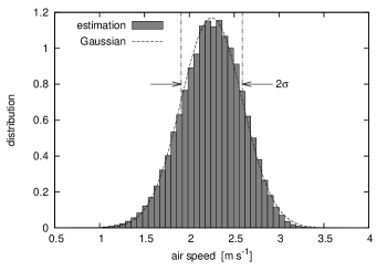
Figure 5: The distribution of the air speed measured in the free jet experiment (see Renner et al.,, 2001). The dashed line corresponds to a Gaussian curve with mean 2.25 $\rm m\,s^{-1}$ and standard deviation 0.341 $\rm m\,s^{-1}$

Renner et al., (2001) measured the air speed in an air into air round free jet experiment. The acquired data series is an example of stationary laboratory turbulence. Figure 5 shows the distribution of the air speed in the free jet experiment which is in good agreement with a Gaussian shaped curve. In other words, the shown histogram corresponds to one slice of the three-dimensional plots in figure 4.

As a conclusion, analysing a period $\vartheta-\Delta\vartheta/2\leq n<\vartheta+\Delta\vartheta/2$ of ABL wind speed data reveals that the distribution of the fluctuation $f^{(m)}_{n}$ around the mean speed $\bar{x}^{(m)}_{n}=V$ is well described by a symmetric Gaussian distribution with a standard deviation being proportional to $V$. The proportionality factor $a(\vartheta,m)$ can be estimated by evaluating the standard deviation of the normalised fluctuation $f^{(m)}_{n}/\bar{x}^{(m)}_{n}$ over the period of interest.

In a further study, we propose a stochastic process which can be used to generate a time series having the same fluctuation behaviour as ABL wind speed data. The work is still in progress.

Additionally, a conclusion about wind speed increments $x_{s;n}=x_{n+s}-x_{n}$ for sufficient large $s$ can be drawn. If $x_{n+s}$ and $x_{n}$ can be treated as being independent from each other and choosing $m$ such that $\bar{x}^{(m)}_{n}\approx\bar{x}^{(m)}_{n+s}$, the increment $x_{s;n}$ is of a symmetric normal distribution with a standard deviation being proportional to $\bar{x}^{(m)}_{n}$. Taking the statistics of $x_{s;n}$ over a much larger time period than the time scale on which $\bar{x}^{(m)}_{n}$ changes, e.g. 24 h, the increment distribution $p_{s}(x_{s})$ corresponds to a superposition of symmetric Gaussians with different volatilities. The variance of the volatilities is determined by the variance of $\bar{x}^{(m)}_{n}$. It (nearly) vanishes if $\bar{x}^{(m)}_{n}\sim{\rm const}$ in time making $p_{s}(x_{s})$ coincide with a Gaussian distribution. Otherwise, $p_{s}(x_{s})$ is fat tailed.

The following two sections intend to analyse the increment series, its statistics, and its limit for large increment lengths.

3 Increment Statistics

This section is dedicated to the statistics of wind speed increments. The increment series is defined as

$$x_{s;n}=x_{n+s}-x_{n}$$ (17)

with $s$ denoting the time over which the increment is measured—the increment length.

Castaing et al., (1990) deduced an analytical expression for the marginal increment distribution $p_{s}(x_{s})$ from the assumption of a log-normally distributed energy transfer rate in turbulence. Castaing’s hypothesis assumes that the increment series in a small time window is of a Gaussian distribution

$$p(x_{s}|\beta)=\sqrt{\frac{\beta}{2\pi}}{\rm e}^{-\frac{\beta}{2}x_{s}^{2}}.$$ (18)

In each window the parameter $\beta$ can be regarded as being constant. However, it varies between the windows according to the log-normal distribution

$$f_{s}(\beta)=\frac{1}{\sqrt{2\pi}\lambda_{s}\beta}{\rm e}^{-\frac{1}{2}\left(\frac{1}{\lambda_{s}}\ln\frac{\beta}{\beta_{s}}\right)^{2}}.$$ (19)

As a result, the increment distribution of ABL wind speed is given by

$$p_{s}(x_{s}) =\int_{0}^{\infty}{\rm d}\beta\,f_{s}(\beta)\,p(x_{s}|\beta)$$

$$=\frac{1}{2\pi\lambda_{s}}\int_{0}^{\infty}{\rm d}\beta\frac{1}{\sqrt{\beta}}{\rm e}^{-\frac{1}{2}\left(\frac{1}{\lambda_{s}}\ln\frac{\beta}{\beta_{s}}\right)^{2}-\frac{1}{2}\beta x_{s}^{2}}.$$ (20)

It is symmetric, leptokurtic, and described by two positive parameters $\beta_{s}$ and $\lambda_{s}$ which are called position and shape parameter, respectively. The latter is directly related to the kurtosis of the increment series by

$$k_{s}=\frac{\left\langle x_{s}^{4}\right\rangle}{\left\langle x_{s}^{2}\right\rangle^{2}}=3{\rm e}^{\lambda_{s}^{2}}>3$$ (21)

so that the shape parameter can be estimated using

$$\lambda_{s}^{2}=\ln\frac{k_{s}}{3}.$$ (22)

The position parameter of the increment process can be estimated via the variance and kurtosis by

$$\beta_{s}=\frac{1}{\sigma_{s}^{2}}\sqrt{\frac{k_{s}}{3}}.$$ (23)

In the limit of $\lambda^{2}_{s}\to 0$ the volatility distribution $f_{s}(\beta)$ in (19) turns into

$$f_{s}(\beta)\overset{\lambda^{2}_{s}\to 0}{\longrightarrow}\delta(\beta-\beta_{s})$$ (24)

making the increment distribution coincide with a Gaussian distribution with variance $\sigma_{s}^{2}=1/\beta_{s}$ and kurtosis $k_{s}=3$:

$$p_{s}(x_{s})\overset{\lambda^{2}_{s}\to 0}{\longrightarrow}\sqrt{\frac{\beta_{s}}{2\pi}}{\rm e}^{-\frac{\beta_{s}}{2}x_{s}^{2}}.$$ (25)

Figure 6: Increment histograms $p_{s}(x_{s})$ for day 186 (left), day 191 (centre), and day 192 (right) of the Lammefjord, (1987) measurement. The normalised histograms are drawn with points whereas the solid lines represent a Castaing distribution with the same variance and kurtosis as the increment series. The histograms are shifted and drawn in a semi-logarithmic plot for better visibility

Figure 6 depicts the increment distribution $p_{s}(x_{s})$ for a variety of $s$ and for three different days (day 186, 191, and 192) of the Lammefjord, (1987) measurement. The fitted Castaing distributions according to (22) and (23) are drawn with solid lines. It can be seen that the empirical histograms are in good agreement with Castaing distributions. Furthermore, the histograms for the data acquired at the days 191 and 192 approach a Gaussian distribution as $s$ becomes larger.

Figure 7: The position parameter $\beta_{s}$ and shape parameter $\lambda^{2}_{s}$ as a function of $s$ for the days 186, 191, and 192 of the Lammefjord, (1987) measurement are plotted in the upper and lower panel, respectively

The intermittency hypothesis and the conclusion drawn in Sec. 2 imply that the shape parameter $\lambda^{2}_{s}$ decreases as $s$ gets larger. In case of (nearly) stationary turbulence it converges to zero, i.e.

$$\lambda^{2}_{s}\overset{s\to\infty}{\longrightarrow}0.$$ (26)

Boettcher et al., (2003) obtained results from laboratory and ABL turbulence showing (26). Consequently, with increasing $s$ both the kurtosis $k_{s}$ and inverse variance $1/\sigma_{s}^{2}$ decrease causing the position parameter to decrease, too. Figure 7 depicts $\beta_{s}$ vs. $s$ and $\lambda^{2}_{s}$ vs. $s$ for the increment distributions of the Lammefjord ABL wind speed data. It can be seen that the shape parameter $\lambda^{2}_{s}$ of the days 191 and 192 goes to zero as $s$ becomes larger whereas it does not reach zero for the day 186 data. In other words, the data acquired at day 186 have leptokurtic increment distributions at large increment lengths.

It is worth mentioning that for laboratory turbulence the empirical increment histograms are in perfect agreement with the hypothetical Castaing shaped curves (see Renner et al.,, 2001, figure 8). Additionally, laboratory turbulence data yield a shape parameter which decreases with $s$ according to a power law and approaches zero for sufficiently large $s$ (see Renner et al.,, 2001, figure 9).

As a summary, this simple approach showed an agreement between the empirical histograms and the hypothetical distributions. The effect of increasing Gaussianity and hence decreasing shape parameter for increasing $s$ can be seen and is well supported by the intermittency hypothesis of idealised turbulence.

Some measurements show a fat tailed increment distribution even for large increment lengths $s$. According to Boettcher et al., (2007) and the conclusion drawn in Sec. 2, a fluctuating mean wind speed might be the reason for this behaviour. It is however the drawback of this technique not being suitable to verify a connection between this kind of non-stationarity and the shape of increment distributions.

4 Superstatistics

We scrutinise the increment series a little further in order to understand the different increment statistics behaviour of ABL wind. The method which this section has its focus on aims to validate the Castaing hypothesis (20) in another way: by computing the, a priori unknown, distribution $f_{s}(\beta)$ and comparing it with a log-normal distribution.

The concept of superposing two statistics was generalised by Beck and Cohen, (2003) and called “superstatistics”. It describes a driven non-equilibrium system of an intensive parameter $\beta$, which in our case is the inverse volatility, fluctuating on a large spatio-temporal scale $T$ whereas the system itself changes on a short spatio-temporal scale $\tau\ll T$.

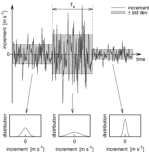
Figure 8: Schematic sketch of the superstatistical approach. The increment series is considered to consist of successive normally distributed segments of length $T_{s}$. Within such a period the mean is considered to be zero and the standard deviation (std dev) approximated by the estimation over the interval

Based on this idea Beck et al., (2005) and Queiros, (2007) proposed an algorithm to approximate the volatility by being piece-wise constant, namely $1/\beta$, and treat the increment series as being of a Gaussian distribution in each segment. Figure 8 sketches schematically the approximation.

We use this algorithm to estimate the statistics of $\beta$ from the increment series $(x_{s;n})_{n=0}^{N-1}$ of ABL wind speed data. The essential step is to find the large time scale $T_{s}$ and estimate $\beta$ in each segment.

Figure 9: Mean window kurtosis as function of the window size $m$ for different increment length $s$ of the ABL wind speed measurement at the Lammefjord, (1987) site. The dashed line corresponds to $\kappa=3$. The intersection $\kappa_{s}^{(m)}=3$ is an estimation for the large time scale shown in figure 10

The large time scale can be identified with the scale on which the increment series is of a normal distribution. Hence, being a measure for Gaussianity, the sample kurtosis of a population ${\cal A}$ is defined as

$$\mathbb{K}{\rm urt}\,{\cal A}=|{\cal A}|\times\frac{\sum_{a\in{\cal A}}(a-\bar{a})^{4}}{\left(\sum_{a\in{\cal A}}(a-\bar{a})^{2}\right)^{2}}$$ (27)

with $\bar{a}=\frac{1}{|{\cal A}|}\sum_{a\in{\cal A}}a$ denoting the sample average and $|{\cal A}|$ denoting the sample size. If the population stems from a Gaussian distributed population, the kurtosis equals to three if the population size is reasonably large. The above defined sample kurtosis is biased with respect to the sample size. If ${\cal A}$ consists of only one or two elements, i.e. ${\cal A}=\{a\}$ or ${\cal A}=\{a_{1},a_{2}\}$, the sample kurtosis $\mathbb{K}{\rm urt}\,{\cal A}=1$. In order to find the large time scale, the increment series $(x_{s;n})_{n=0}^{N-1}$ is split into $N_{m}$ sub-series: ${\rm int}\left[N/m\right]$ sub-series of size $m$ and if necessary one remaining sub-series of size less than $m$. For each sub-series the sample kurtosis is computed. The average of the $N_{m}$ sub-series kurtosis is taken as measure of sub-series Gaussianity. Changing $m$ means changing the length of the sub-series so that we arrive at the mean sub-series kurtosis written as

$$\kappa^{(m)}_{s}=\left\langle\mathbb{K}{\rm urt}\left\{x_{s;km},\dots,x_{s;(k+1)m-1}\right\}\right\rangle_{k=0,\dots,N_{m}-1}$$ (28)

being a function of the window length $m$. As mentioned above, $\kappa^{(m)}_{s}=1$ for $m\leq 2$ . As $m$ gets larger $N_{m}$ tends to one. This results in a $\kappa^{(m)}_{s}$ being equal to the sample kurtosis of the whole increment series whose kurtosis is larger than three because we know from the increment statistics that the increment series is of a leptokurtic distribution. Hence, somewhere between $1<m<N$ there is a value $m$ where $\kappa^{(m=T_{s})}_{s}$ is closest to three,

$$\kappa^{(m=T_{s})}_{s}=3,$$ (29)

which, according to Beck et al., (2005) and Queiros, (2007), is taken as an estimation for the large time scale $T_{s}$. Figure 9 displays the mean window kurtosis as function of the window size $m$ for different increment lengths $s$ for the ABL wind speed measurement at the Lammefjord, (1987) site. It can be seen that it increases with increasing $m$ and has an intersection with three.

As $T_{s}$ is supposed to be large there should be no problem with using the biased kurtosis estimator defined above. Using an unbiased estimator would give curves like $\kappa^{(m)}_{s}\approx 3$ for $m<T_{s}$ and $\kappa^{(m)}_{s}>3$ for $m>T_{s}$. From a statistical point of view it is more involved to find the point $T_{s}$ that way making the algorithm unnecessarily more complicated.

Knowing the length $T_{s}$ of the sub-series such that they show in average Gaussian behaviour, leads to the question whether the relaxation time of the process is small compared to $T_{s}$. It is reflected by the short time scale $\tau_{s}$ being estimated by the decay of the auto correlation function $\gamma_{s;t}$:

$$\tau_{s}=\min_{t=1,...,N-1}\{t:\gamma_{s;t}\leq{\rm e}^{-1}\}.$$ (30)

If $\tau_{s}$ is much smaller than $T_{s}$ the existence of two separated time scales is justified so that it is suitable to estimate the the variance in each sub-series of length $T_{s}$ by its (unbiased) sample variance and identify its inverse as

$$\beta_{k}=\frac{1}{\mathbb{V}{\rm ar}\left\{x_{s;kT_{s}},\dots,x_{s;(k+1)T_{s}-1}\right\}}.$$ (31)

Its estimated distribution reads

$$f_{s}(\beta)=\left\langle\delta(\beta-\beta_{k})\right\rangle_{k}$$ (32)

which, hypothetically, has the shape of a log-normal distribution. Thus, it is more convenient to consider the variables

$$\Lambda_{k}=\ln\beta_{k}$$ (33)

and their estimated distribution

$$h_{s}(\Lambda)=\left\langle\delta(\Lambda-\Lambda_{k})\right\rangle_{k}.$$ (34)

The hypothesis reads

$$H_{0}:\quad h_{s}(\Lambda)=\frac{1}{\sqrt{2\pi}\lambda_{s}}{\rm e}^{-\frac{1}{2}\left(\frac{\Lambda-\Lambda_{s}}{\lambda_{s}}\right)^{2}}$$ (35)

with $\Lambda_{s}=\ln\beta_{s}$ turning (20) into

$$p_{s}(x_{s})=\frac{1}{2\pi\lambda_{s}}\int_{-\infty}^{\infty}{\rm d}\Lambda\,{\rm e}^{-\frac{1}{2}\left\{\left(\frac{\Lambda-\Lambda_{s}}{\lambda_{s}}\right)^{2}-\Lambda+x_{s}^{2}{\rm e}^{\Lambda}\right\}}.$$ (36)

This approach provides an alternative way to fit the Castaing parameters by

$$\ln\beta_{s}=\Lambda_{s}=\mathbb{M}{\rm ean}\left\{\Lambda_{0},\dots,\Lambda_{N_{\Lambda;s}-1}\right\}$$ (37)

and

$$\lambda_{s}^{2}=\mathbb{V}{\rm ar}\left\{\Lambda_{0},\dots,\Lambda_{N_{\Lambda;s}-1}\right\}.$$ (38)

Figure 10: The top and central panel show the estimated large and short time scales, $T_{s}$ and $\tau_{s}$ in time steps, respectively, for three 24 h data acquired at the Lammefjord, (1987) site (day 186, 191, and 192). A day consists of 691200 data points being the upper limit for the estimation of $T_{s}$. The central panel displays the short time scale $\tau_{s}$ which is estimated by the decay of the auto correlation function for small lags. The ratio $T_{s}/\tau_{s}$ is depicted in the lowest panel

Figure 10 shows the estimated large and short time scale of wind speed increment data acquired at the Lammefjord, (1987) site as a function of $s$ in its top and central panel, respectively. $T_{s}$, whose estimation is bounded from above by the number of points which the time series consists of, generally increases with increasing $s$. It describes the scale on which the increment process is of a normal distribution and is hence a measure for Gaussianity. Therefore, an increasing large time scale is in full agreement with the approach to Gaussianity as the increment length gets larger. Additionally, the comparably slow approach to Gaussianity of the data gathered at day 186 can be recovered, cf. figure 7. The plot in the lowest panel of figure 10 verifies the existence of two separated time scales. It visualises the ratio $T_{s}/\tau_{s}$ being of the order of magnitude of 10 or larger.

The series $(\Lambda_{k})_{k=0}^{N_{\Lambda;s}-1}$ for the Lammefjord day 191 data is computed according to (31) and (33). Figure 11 shows exemplarily that the estimated distribution $h_{s}(\Lambda)$ for $s=8$ is close to Gaussian. But it has a systematic and statistically significant deviation. In fact, it has a positive skewness. The non-Gaussianity is underlined by the quantile-quantile plot in the top right panel of this figure. However, the increment distribution is in good agreement with a Castaing shaped distribution, cf. figure 6. This allows the statement that the superstatistical approach is sensitive enough to discover small deviations from Castaing’s hypothesis.

Figure 11: The top left panel displays the estimated 24 h $\Lambda$-distribution $h_{s}(\Lambda)$ for $s=8$ of the Lammefjord, (1987) measurement day 191. $h_{s}^{*}(\Lambda)$ denotes a Gaussian distribution with mean $\left\langle\Lambda\right\rangle$ and variance $\left\langle(\Lambda-\left\langle\Lambda\right\rangle)^{2}\right\rangle$. The quantile-quantile plot is shown in the upper right panel. The bottom panel displays the $\Lambda$-series for that day. The numbers 1 to 12 illustrate the twelve 2 h sub-samples which are individually investigated with respect to superstatistics

Figure 12: The top (central) panel shows the mean (variance) of $\Lambda$ for each sub-sample of the data acquired at day 191 at the Lammefjord, (1987) site and for several $s$. The mean and variance can be identified with the position and shape parameter, respectively. The solid line corresponds to $s=8$ and is therefore related to the graphs in figure 11. The test value of the Kolmogorov-Smirnov test, $d^{\rm KS}_{s}(\vartheta)\times\sqrt{N_{\Lambda;s}(\vartheta)}$, is plotted in the lowest panel. The dashed line corresponds to the critical value for the significance level $\alpha=1~{}\%$

Boettcher et al., (2007) showed that the distribution of ABL wind speed increments can be understood as a superposition of different subsets of isotropic turbulence. Indeed, the depicted $\Lambda$-series in the lowest panel of figure 11 indicates that the hypothesis “$\Lambda$ is of a normal distribution” might be fulfilled on a smaller period than 24 h. Hence, the 24 h increment series $(x_{s;n})_{n=0}^{N-1}$ was divided into twelve 2 h sub-samples where each of which represents a time $\vartheta$ of the day. Each sub-sample was analysed with respect to superstatistics individually. After computing and comparing the time scales $T_{s}(\vartheta)$ and $\tau_{s}(\vartheta)$, the $\Lambda$-series for each sub-sample around $\vartheta$ was extracted and tested for the hypothesis of being normally distributed. This test was done using a Kolmogorov-Smirnov test (see e.g. Daniel,, 1990, chapter 8). Its test value corresponds to the largest deviation of the empirical cumulative distribution function (c.d.f.) $S_{s}(\Lambda,\vartheta)$ from the corresponding Gaussian c.d.f. $\Phi_{0}\left(\frac{\Lambda-\Lambda_{s}(\vartheta)}{\lambda_{s}(\vartheta)}\right)$ with fitted $\Lambda_{s}(\vartheta)$ and $\lambda_{s}^{2}(\vartheta)$. It is denoted by

$$d^{\rm KS}_{s}(\vartheta)=\sup_{\Lambda}\left|S_{s}(\Lambda,\vartheta)-\Phi_{0}\left(\frac{\Lambda-\Lambda_{s}(\vartheta)}{\lambda_{s}(\vartheta)}\right)\right|.$$ (39)

The hypothesis $H_{0}$ in (35) is rejected on a significance level $\alpha$ if

$$d^{\rm KS}_{s}(\vartheta)\times\sqrt{N_{\Lambda;s}(\vartheta)}\geq d^{\rm KS}_{\rm crit}(\alpha).$$ (40)

The critical value is 1.63 for $\alpha=1\,\%$ and $N_{\Lambda;s}(\vartheta)>40$ where the latter denotes the number of data points in the $\Lambda$-series for increment length $s$ and time $\vartheta$ (see e.g. Daniel,, 1990, table A.18 for tabulated values).

Figure 12 shows the results for each 2 h sub-sample of the Lammefjord day 191 data plotted as a function of time $\vartheta$ for a variety of increment lengths $s$. The top and central panel depict the mean and variance of $\Lambda$ for each sub-sample, respectively. According to (37) and (38) they can be identified with $\Lambda_{s}=\ln\beta_{s}$ and $\lambda_{s}^{2}$, respectively. The bottom panel shows the test value of the Kolmogorov-Smirnov test and the critical value for the significance level $\alpha=1~{}\%$. The graph allows the conclusion that the hypothesis “the $\Lambda$-series of each sub-sample around $\vartheta$ and for different $s$ is of a normal distribution” can not be rejected on a significance level $\alpha=1~{}\%$. Moreover, the $\lambda_{s}^{2}$-plots in the central panel reveal that for large $s$ the shape parameter of each sub-sample approaches zero as it is expected from the intermittency hypothesis. Therefore, it can be concluded that Castaing’s hypothesis is fulfilled during time intervals of 2 h. But it is violated on larger time scales, such as 24 h, due to non-stationarity which are reflected by the time dependence of $\Lambda_{s}(\vartheta)$ and $\lambda_{s}^{2}(\vartheta)$. In other words, the distribution shown in figure 11 is a superposition of Gaussians with different means $\Lambda_{s}(\vartheta)$ and variances $\lambda_{s}^{2}(\vartheta)$ for $s=8$ and is thus not exactly a normal shaped distribution.

Figure 13: The top left panel displays the estimated 24 h $\Lambda$-distribution $h_{s}(\Lambda)$ for $s=8$ of the Lammefjord, (1987) measurement day 186. $h_{s}^{*}(\Lambda)$ denotes a Gaussian distribution with mean $\left\langle\Lambda\right\rangle$ and variance $\left\langle(\Lambda-\left\langle\Lambda\right\rangle)^{2}\right\rangle$. The quantile-quantile plot is shown in the upper right panel. The bottom panel displays the $\Lambda$-series for that day. The numbers 1 to 12 illustrate the twelve 2 h sub-samples which are individually investigated with respect to superstatistics

Figure 14: The top (central) panel shows the mean (variance) of $\Lambda$ for each sub-sample of the data acquired at day 186 at the Lammefjord, (1987) site and for several $s$. The mean and variance can be identified with the position and shape parameter, respectively. The solid line corresponds to $s=8$ and is therefore related to the graphs in figure 13. The test value of the Kolmogorov-Smirnov test, $d^{\rm KS}_{s}(\vartheta)\times\sqrt{N_{\Lambda;s}(\vartheta)}$, is plotted in the lowest panel. The dashed line corresponds to the critical value for the significance level $\alpha=1~{}\%$

The same analysis was done with the Lammefjord day 186 data which did not show a clear cross-over behaviour in figure 6. The superstatistical algorithm was used to extract the $\Lambda$-series from the 24 h time series $(x_{s;n})_{n=0}^{N-1}$ and tested for Gaussianity. The upper left panel of figure 13 shows the histogram $h_{s}(\Lambda)$ for $s=8$ which is clearly non-Gaussian shaped. This explains the small deviation of $p_{s}(x_{s})$ in figure 6 from the fitted Castaing distribution for $s=8$. The 24 h increment series $(x_{s;n})_{n=0}^{N-1}$ was also divided into twelve 2 h sub-samples where each of which was analysed with respect to superstatistics individually. Figure 14 shows the Castaing parameters $\Lambda_{s}(\vartheta)$ and $\lambda^{2}_{s}(\vartheta)$ as a function of time $\vartheta$. The time span $8~{}{\rm h}\lesssim\vartheta\lesssim 18~{}{\rm h}$ is the only region where Castaing’s hypothesis can not be rejected on a 2 h scale with $\alpha=1~{}\%$: the Kolmogorov-Smirnov test value $d^{\rm KS}_{s}(\vartheta)\times\sqrt{N_{\Lambda;s}(\vartheta)}$ is below the critical value and the shape parameter $\lambda^{2}_{s}(\vartheta)$ goes to zero as $s$ gets larger. That means that both Castaing’s hypothesis and the cross-over behaviour can be recovered in the mentioned time span on windows of 2 h period. Outside this region, the length of 2 h for the sub-samples is still too large or in other words the resolution is too low for recovering a normally distributed $\Lambda$-series. However, going to smaller sub-samples gives worse statistics due to the reduced number of data points in each sub-sample. Nevertheless, the increments of this day are much more non-stationary than the data gathered at day 191. It exemplifies that high non-stationarity of wind speed data cause a fat tailed increment distribution for large increment length $s$.

The data acquired at day 192 at the Lammefjord site show similar behaviour to the day 191 data when analysed with respect to superstatistics.

As a summary, the superstatistical approach is sensitive enough to detect sub-regions of the increment series where Castaing’s hypothesis is fulfilled. In such a region the increment distribution takes the shape given in (36). The position and shape parameter change with time as they differ between different sub-regions. This makes this approach be capable of determining the dynamics of $\Lambda_{s}(\vartheta)=\ln\beta_{s}(\vartheta)$ and $\lambda^{2}_{s}(\vartheta)$. Moreover, it can be used to verify that wind speed data with large fluctuating Castaing parameters have a non-Gaussian increment distribution at large increment lengths.

5 Conclusions

Our study verified the picture of natural ABL turbulence to be composed of successively occurring close to ideal turbulence with different parameters.

We showed that in good approximation the fluctuation of the the wind speed around its window average $V$ is of a symmetric normal distribution with a standard deviation being proportional to $V$. The proportionality factor can be estimated by the standard deviation of the normalised fluctuation. The investigation of the time dependent volatility of the normalised fluctuation leads to the time resolution of the proportionality factor. Our analysis showed that approximating it by being constant over 24 h is reasonable. However, within 24 h the mean wind speed changed frequently leading to two separate time scales: the time scale on which the mean wind speed changes and the time scale on which the proportionality factor between the mean wind speed and the standard deviation of the fluctuation can be approximated as being constant. The mean speed of stationary laboratory turbulence does not alter with time so that the $V$ dependence of the fluctuation distribution can not be investigated by means of such experiments. Nevertheless, the fluctuation is of a normal distribution, too, leading to the conclusion that ABL turbulence is a sequence of stationary turbulence with varying mean.

The intermittency behaviour of ABL wind speed was tested using the increment statistics approach. The coincidence between the empirical histograms and the hypothetical distributions makes the increment series in this representation look stationary. However, Castaing’s intermittency hypothesis involves a time scale separation. On a small scale the wind speed increments are of a symmetric normal distribution whose variance alters on a larger scale according to a log-normal distribution.

We checked this time scale separation using a superstatistical approach. We found that there is a “critical” time scale below which the increment series behaves normally distributed and above which the increment series is of a leptokurtic distribution. In the terminology of superstatistics this time scale is referred to as the large time scale in contrast to the small time scale reflecting the relaxation time of the increment process. If the latter is small compared to the large time scale it is possible to estimate the variance of each Gaussian segment and analyse their statistics. We found that their logarithm is not exactly of a stationary normal distribution but rather of a sequence of normal distributions with varying mean and variance. This incorporates a third time scale into the ABL wind speed increment series on which the log-normal distribution of the variances in the sense of Castaing’s hypothesis can be approximated as being stationary.

We additionally verified that highly non-stationary turbulence might show a fat tailed increment distribution even at large increment length $s$.

Acknowledgements.

The study was supported by Germany’s Federal Ministry for Education and Research (BMBF) under grant number 03SF0314. It is part of the joint project “Statistical analysis and stochastic modelling of turbulent gusts in surface wind”.

References

- Beck et al., (2005) Beck, C., Cohen, E., and Swinney, H. (2005). From time series to superstatistics. Phys. Rev. E, 72:056133.
- Beck and Cohen, (2003) Beck, C. and Cohen, E. G. D. (2003). Superstatistics. Physica A, 322:267–275.
- Boettcher et al., (2007) Boettcher, F., Barth, S., and Peinke, J. (2007). Small and large scale fluctuations in atmospheric wind speeds. Stoch. Environ. Res. Risk Assess., 21:299–308.
- Boettcher et al., (2003) Boettcher, F., Renner, C., Waldl, H. P., and Peinke, J. (2003). On the statistics of wind gusts. Bound.-Layer Meteor., 108:163–173.
- Burton et al., (2004) Burton, T., Sharpe, D., Jenkins, N., and Bossanyi, E. (2004). Wind Energy Handbook. John Wiley.
- Castaing et al., (1990) Castaing, B., Gagne, Y., and Hopfinger, E. J. (1990). Velocity probability density-functions of high Reynolds number turbulence. Physica D, 46:177–200.
- Daniel, (1990) Daniel, W. (1990). Applied Nonparametric Statistics. PWS-Kent, second edition.
- (8) Kolmogorov, A. N. (1941a). Dissipation of energy in locally isotropic turbulence. Dokl. Akad. Nauk SSSR, 32:16–18.
- (9) Kolmogorov, A. N. (1941b). The local structure of turbulence in incompressible viscous fluid for very large Reynolds number. Dokl. Akad. Nauk SSSR, 30:299–303.
- Kolmogorov, (1962) Kolmogorov, A. N. (1962). A refinement of previous hypotheses concerning the local structure of turbulence in a viscous incompressible fluid at high Reynolds number. J. Fluid Mech., 13:82–85.
- Lammefjord, (1987) Lammefjord (1987). Lammefjord data obtained from the Risø National Laboratory in Denmark, http://www.risoe.dk/vea, through http://www.winddata.com.
- Obukhov, (1962) Obukhov, A. (1962). Some specific features of atmospheric turbulence. J. Fluid Mech., 13:77–81.
- Queiros, (2007) Queiros, S. M. D. (2007). On new conditions for evaluate long-time scales in superstatistical time series. Physica A, 385:191–198.
- Renner et al., (2001) Renner, C., Peinke, J., and Friedrich, R. (2001). Experimental indications for Markov properties of small-scale turbulence. J. Fluid Mech., 433:383–409.
- Taylor, (1938) Taylor, G. (1938). The spectrum of turbulence. Proc. R. Soc. Lond. A, 164:476–490.
- Wallace and Hobbs, (2006) Wallace, J. M. and Hobbs, P. V. (2006). Atmospheric Science. Academic Press Elsevier, second edition.