The first digit frequencies of primes and Riemann zeta zeros tend to uniformity following a size-dependent generalized Benford’s law

Abstract

first significant digit, Benford’s law, prime number, pattern, zeta function. Prime numbers seem to distribute among the natural numbers with no other law than that of chance, however its global distribution presents a quite remarkable smoothness. Such interplay between randomness and regularity has motivated scientists of all ages to search for local and global patterns in this distribution that eventually could shed light into the ultimate nature of primes. In this work we show that a generalization of the well known first-digit Benford’s law, which addresses the rate of appearance of a given leading digit $d$ in data sets, describes with astonishing precision the statistical distribution of leading digits in the prime numbers sequence. Moreover, a reciprocal version of this pattern also takes place in the sequence of the nontrivial Riemann zeta zeros. We prove that the prime number theorem is, in the last analysis, the responsible of these patterns. Some new relations concerning the prime numbers distribution are also deduced, including a new approximation to the counting function $\pi(n)$. Furthermore, some relations concerning the statistical conformance to this generalized Benford’s law are derived. Some applications are finally discussed.

1 Introduction

The individual location of prime numbers within the integers seems to be random, however its global distribution exhibits a remarkable regularity (Zagier 1977). Certainly, this tenseness between local randomness and global order has lead the distribution of primes to be, since antiquity, a fascinating problem for mathematicians (Dickson 2005) and more recently for physicists (see for instance Berry et al. 1999, Kriecherbauer et al 2001, Watkins). The Prime Number Theorem, that addresses the global smoothness of the counting function $\pi(n)$ providing the number of primes less or equal to integer $n$, was the first hint of such regularity (Tenenbaum 2000). Some other prime patterns have been advanced so far, from the visual Ulam spiral (Stein et al 1964) to the arithmetic progression of primes (Green et al 2008), while some others remain conjectures, like the global gap distribution between primes or the twin primes distribution (Tenenbaum 2000), enhancing the mysterious interplay between apparent randomness and hidden regularity. There are indeed many open problems to be solved, and the prime number distribution is yet to be understood (see for instance Guy 2004, Ribenboim 2004, Caldwell). For instance, there exist deep connections between the prime number sequence and the nontrivial zeros of the Riemann zeta function (Watkins, Edwards 1964). The celebrated Riemann Hypothesis, one of the most important open problem in mathematics, states that the nontrivial zeros of the complex-valued Riemann zeta function $\zeta(s)=\sum_{n=1}^{\infty}1/n^{s}$ are all complex numbers with real part $1/2$, the location of these being intimately connected with the prime number distribution (Edwards 1964, Chernoff 2000).
Here we address the statistics of the first significant or leading digit of both the sequences of primes and the sequence of Riemann nontrivial zeta zeros. We will show that while the first digit distribution is asymptotically uniform in both sequences (that is to say, integers $1,...,9$ tend to be equally likely first digits in both sequences when we take into account the infinite amount of them), this asymptotic uniformity is reached in a very precise trend, namely by following a size-dependent Generalized Benford’s law, what constitutes an as yet unnoticed pattern in both sequences. The rest of the paper is organized as follows: in section 2 we introduce the most celebrated first digit distribution: the Benford’s law. In section 3 we introduce a generalization of the Benford’s law, and we show that both the prime numbers and Riemann zeta zeros sequences follow what we call a size-dependent Generalized Benford’s law, introducing two unnoticed patterns of statistical regularity. In section 4 we point out that the mean local density of both sequences is the responsible of these latter patterns. We provide both statistical arguments (statistical conformance between distributions) and analytical developments (asymptotic expansions) that support our claim. In section 5 we conclude and discuss on the possible applications.

2 Benford’s law

The leading digit of a number stands for its non-zero leftmost digit. For instance, the leading digits of the prime $7703$ and the zeta zero $21.022...$ are $7$ and $2$ respectively. The most celebrated leading digit distribution is the so called Benford’s law (Hill 1996), after physicist Frank Benford (1938) who empirically found that in many disparate natural data sets and mathematical sequences, the leading digit $d$ wasn’t uniformly distributed as might be expected, but instead had a biased probability of appearance

$$P(d)=\log_{10}(1+1/d),$$ (1)

where $d=1,2,\dots,9$. While this empirical law was indeed firstly discovered by astronomer Simon Newcomb (1881), it is popularly known as the Benford’s law or alternatively as the Law of Anomalous Numbers. Several disparate data sets such as stock prices, freezing points of chemical compounds or physical constants exhibit this pattern at least empirically. While originally being only a curious pattern (Raimi 1976), practical implications began to emerge in the 1960s in the design of efficient computers (see for instance Knuth 1967). In recent years goodness-of-fit test against Benford’s law has been used to detect possible fraudulent financial data, by analyzing the deviations of accounting data, corporation incomes, tax returns or scientific experimental data to theoretical Benford predictions (Nigrini 2000). Indeed, digit pattern analysis can produce valuable findings not revealed by a mere glance, as is the case of recent election results (Mebane 2006, Nigrini 2000).

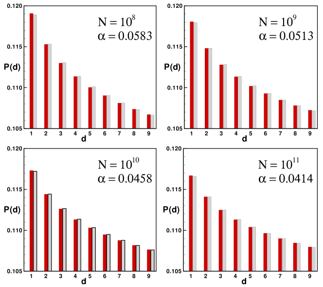
Figure 1: Leading digit histogram of the prime number sequence. Each plot represents, for the set of prime numbers comprised in the interval $[1,N]$, the relative frequency of the leading digit $d$ (red bars). Sample sizes are: $5761455$ primes for $N=10^{8}$, $50847534$ primes for $N=10^{9}$, $455052511$ primes for $N=10^{10}$ and $4118054813$ primes for $N=10^{11}$. Grey bars represent the fitting to a Generalized Benford distribution (eq. 2) with a given exponent $\alpha(N)$.

Many mathematical sequences such as $(n^{n})_{n\in\mathbb{N}}$ and $(n!)_{n\in\mathbb{N}}$ (Benford 1938), binomial arrays $(^{n}_{k})$ (Diaconis 1977), geometric sequences or sequences generated by recurrence relations (Raimi 1976, Miller et al. 2006) to cite a few are proved to be Benford. One may thus wonder if this is the case for the primes. In figure 1 we have plotted the leading digit $d$ rate of appearance for the prime numbers placed in the interval $[1,N]$ (red bars), for different sizes $N$. Note that intervals $[1,N]$ have been chosen such that $N=10^{D},\ D\in\mathbb{N}$ in order to assure an unbiased sample where all possible first digits are equiprobable a priori (see the appendix for further details). Benford’s law states that the first digit of a series data extracted at random is $1$ with a frequency of $30.1\%$, and is $9$ only about $4.6\%$. Note in figure 1 that primes seem however to approximate uniformity in its first digit. Indeed, the more we increase the interval under study, the more we approach uniformity (in the sense that all integers $1,...,9$ tend to be equally likely as a first digit). As a matter of fact, Diaconis (1977) proved that primes are not Benford distributed as long as their first significant digit is asymptotically uniformly distributed. A question arises straightforwardly: how does the prime sequence reach this uniform behavior in the infinite limit? Is there any pattern on its trend towards uniformity, or on the contrary, does the first digit distribution lacks any structure for finite sets?

3 Generalized Benford’s law: the pattern

Several mathematical insights of the Benford’s law have been also advanced so far (Hill 1995a, Pinkham 1961, Raimi 1976, Miller et al. 2006), and Hill (1995b) proved a Central Limit-like Theorem which states that random entries picked from random distributions form a sequence whose first digit distribution converges to the Benford’s law, explaining thereby its ubiquity. This law has been for a long time practically the only distribution that could explain the presence of skewed first digit frequencies in generic data sets. Recently Pietronero et al. (2001) proposed a generalization of Benford’s law based in multiplicative processes (see also Nigrini et al. 2007). It is well known that a stochastic process with probability density $1/x$ generates data which are Benford, therefore series generated by power law distributions $P(x)\sim x^{-\alpha}$ with $\alpha\neq 1$, would have a first digit distribution that follow a so-called Generalized Benford’s law (GBL):

$$P(d)=C\int_{d}^{d+1}x^{-\alpha}dx=\frac{1}{10^{1-\alpha}-1}\bigg{[}(d+1)^{1-\alpha}-d^{1-\alpha}\bigg{]},$$ (2)

where the prefactor is fixed for normalization to hold and $\alpha$ is the exponent of the original power law distribution (for $\alpha=1$, the GBL reduces to the Benford’s law).

3.1 The pattern in primes

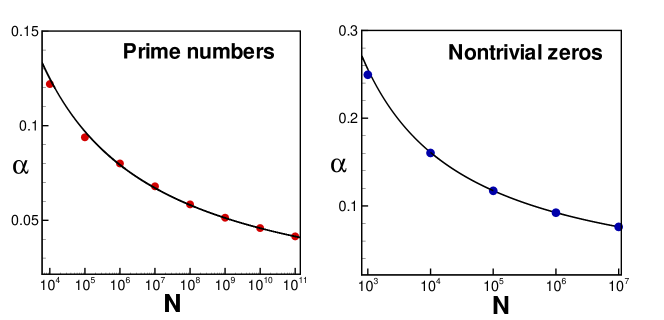
Figure 2: Size dependent parameter $\alpha(N)$. Left: Red dots represent the exponent $\alpha(N)$ for which the first significant digit of prime number sequence fits a Generalized Benford Law in the interval $[1,N]$. The black line corresponds to the fitting, using a least squares method, $\alpha(N)=1/(\log N-1.10)$. Right: same analysis as for the left figure, but for the Riemann nontrivial zeta zeros sequence. The best fitting is $\alpha(N)=1/(\log N-2.92)$.

Although Diaconis showed that the leading digit of primes distributes uniformly in the infinite limit, there exist a clear bias from uniformity for finite sets (see figure 1). In this figure we have also plotted (grey bars) the fitting to a GBL. Note that in each of the four intervals, there is a particular value of exponent $\alpha$ for which an excellent agreement holds (see the appendix for fitting methods and statistical tests). More specifically, given an interval $[1,N]$, there exists a particular value $\alpha(N)$ for which a GBL fits with extremely good accuracy the first digit distribution of the primes appearing in that interval. Interestingly, the value of the fitting parameter $\alpha$ decreases as the interval, hence the number of primes, increases in a very particular way. In the left part of figure 2 we have plotted this size dependence, showing that a functional relation between $\alpha$ and $N$ takes place:

$$\alpha(N)=\frac{1}{\log N-a},$$ (3)

where $a=1.10\pm 0.05$ for large values of $N$. Notice that $\lim_{N\rightarrow\infty}\alpha(N)=0$, and in this situation this size-dependent GBL reduces to the uniform distribution, in consistency with previous theory (Diaconis 1977). Despite the local randomness of the prime numbers sequence, it seems that its first digit distribution converges smoothly to uniformity in a very precise trend: as a GBL with a size dependent exponent $\alpha(N)$.

3.1.1 GBL Extension

At this point an extension of the GBL to include, not only the first significative digit, but the first $k$ significative ones can be done (Hill 1995b). Given a number $n$, we can consider its $k$ first significative digits $d_{1},d_{2}\dots,d_{k}$ through its decimal representation: $D=\sum_{i=1}^{k}{d_{i}10^{k-i}}$, where $d_{1}\in\{1,\dots,9\}$ and $d_{i}\in\{0,1,\dots,9\}$ for $i\geq 2$. Hence, the extended GBL providing the probability of starting with number $D$ is

$$P(d_{1},d_{2},\dots,d_{k})=P(D)$$

$$=\frac{1}{(10^{k})^{1-\alpha}-10^{k-1}}\bigg{[}(D+1)^{1-\alpha}-D^{1-\alpha}\bigg{]}.$$ (4)

Figure 3 represents the fitting of the $4118054813$ primes appearing in the interval $[1,10^{11}]$ to an extended GBL for $k=2,3,4$ and $5$: interestingly, the pattern still holds.

3.2 The ‘mirror’ pattern in the Riemann zeta zeros sequence

Once the pattern has been put forward in the case of the prime number sequence, we may wonder if a similar behavior holds for the sequence of nontrivial Riemann zeta zeros (zeros sequence from now on). This sequence is composed by the imaginary part of the nontrivial zeros (actually only those with positive imaginary part are taken into account by symmetry reasons) of $\zeta(s)$. While this sequence is not Benford distributed in the light of a theorem by Rademacher-Hlawka (1984) that proves that it is asymptotically uniform, will it follow a size-dependent GBL as in the case of the primes?

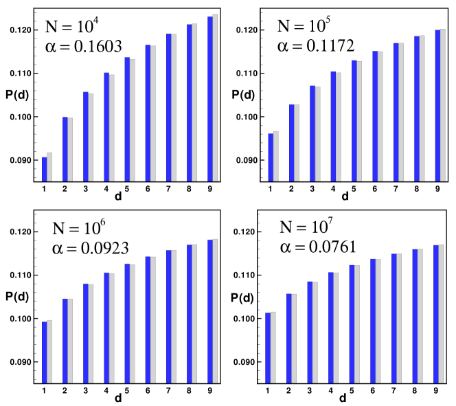
Figure 4: Leading digit histogram of the nontrivial Riemann zeta zeros sequence. Each plot represents, for the sequence of Riemann zeta zeros comprised in the interval $[1,N]$, the observed relative frequency of leading digit $d$ (blue bars). Sample sizes are: $10142$ zeros for $N=10^{4}$, $138069$ zeros for $N=10^{5}$, $1747146$ zeros for $N=10^{6}$ and $21136126$ zeros for $N=10^{7}$. Grey bars represent the fitting to a GBL following equation 5 with a given exponent $\alpha(N)$.

In figure 4 we have plotted, in the interval $[1,N]$ and for different values of $N$, the relative frequencies of leading digit $d$ in the zeros sequence (blue bars), and in grey bars a fitting to a GBL with density $x^{\alpha}$, i.e.:

$$P(d)=C\int_{d}^{d+1}x^{\alpha}dx=\frac{1}{10^{1+\alpha}-1}\bigg{[}(d+1)^{1+\alpha}-d^{1+\alpha}\bigg{]}$$ (5)

(this reciprocity is clarified later in the text). Note that a very good agreement holds again for particular size-dependent values of $\alpha$, and the same functional relation as equation 3 holds with $a=2.92\pm 0.05$. As in the case of the primes, this size dependent GBL tends to uniformity for $N\rightarrow\infty$, as it should (Hlawka 1984). Moreover, the extended version of equation 5 for the $k$ first significative digits is

$$P(d_{1},d_{2},\dots,d_{k})=P(D)$$

$$=\frac{1}{(10^{k})^{1+\alpha}-10^{k-1}}\bigg{[}(D+1)^{1+\alpha}-D^{1+\alpha}\bigg{]}.$$ (6)

As can be seen in figure 5, the pattern also holds in this case.

4 Explanation of the primes pattern

Why do these two sequences exhibit this unexpected pattern in the leading digit distribution? What is the responsible for it to take place? While the prime number distribution is deterministic in the sense that precise rules determine whether an integer is prime or not, its apparent local randomness has suggested several stochastic interpretations. In particular, Cramér (1935, see also Tenembaum 2000) defined the following model: assume that we have a sequence of urns $U(n)$ where $n=1,2,...$ and put black and white balls in each urn such that the probability of drawing a white ball in the $k^{th}$-urn goes like $1/\log k$. Then, in order to generate a sequence of pseudo-random prime numbers we only need to draw a ball from each urn: if the drawing from the $k^{th}$-urn is white, then $k$ will be labeled as a pseudo-random prime. The prime number sequence can indeed be understood as a concrete realization of this stochastic process, where the chance of a given integer $x$ to be prime is $1/\log x$.
We have repeated all statistical tests within the stochastic Cramér model, and have found that a statistical sample of pseudo-random prime numbers in $[1,10^{11}]$ is also GBL distributed and reproduce all statistical analysis previously found in the actual primes (see the appendix for an in-depth analysis). This result strongly suggests that a density $1/\log x$, which is nothing but the mean local primes density by virtue of the prime number theorem, is likely to be the responsible for the GBL pattern. In what follows we will provide further statistical and analytical arguments that support this fact.

4.1 Statistical conformance of prime number distribution to GBL

Recently, it has been shown that disparate distributions such as the Lognormal, the Weibull or the Exponential distribution can generate standard Benford behavior (Leemis et al. 2000) for particular values of their parameters. In this sense, a similar phenomenon could be taking place with GBL: can different distributions generate GBL behavior? One should thus switch the emphasis from the examination of data sets that obey GBL to probability distributions that do so, other than power laws.

4.1.1 $\chi^{2}$-test for conformance between distributions

The prime counting function $\pi(N)$ provides the number of primes in the interval $[1,N]$ (Tenenbaum et al. 2000) and up to normalization, stands as the cumulative distribution function of primes. While $\pi(N)$ is a stepped function, a nice asymptotic approximation is the offset logarithmic integral:

$$\pi(N)\sim\int_{2}^{N}\frac{1}{\log x}dx=\textrm{Li}(N),$$ (7)

(one of the formulations of the Riemann hypothesis actually states that $|\textrm{Li}(n)-\pi(n)|<c\sqrt{n}\log n$, for some constant $c$ (Edwards 1974)). We can interpret $1/\log x$ as an average prime density and the lower bound of the integral is set to be $2$ for singularity reasons. Following Leemis et al. (2000), we can calculate a chi-square goodness-of-fit test of the conformance between the first digit distribution generated by $\textrm{Li}(N)$ and a GBL with exponent $\alpha(N)$. The test statistic is in this case:

$$c=\sum_{d=1}^{9}\frac{[\textrm{Pr}(Y=d)-\textrm{Pr}(X=d)]^{2}}{\textrm{Pr}(X=d)},$$ (8)

where $\textrm{Pr}(X)$ is the first digit probability (eq. 2) for a GBL associated to a probability distribution with exponent $\alpha(N)$ and $\textrm{Pr}(Y)$ is the tested probability. In table 1 we have computed, fixed the interval $[1,N]$, the chi-square statistic $c$ for two different scenarios, namely the normalized logarithmic integral $\textrm{Li}(n)/\textrm{Li}(N)$ and the normalized prime counting function $\pi(n)/\pi(N)$, with $n\in[1,N]$. In both cases there is a remarkable good agreement and we cannot reject the hypothesis that primes are size-dependent GBL.

$N$	$c$ for	$c$ for
	$\pi(x)/\pi(N)$	$\textrm{Li}(x)/\textrm{Li}(N)$
$10^{3}$	$0.59\cdot 10^{-2}$	$0.58\cdot 10^{-2}$
$10^{4}$	$0.86\cdot 10^{-3}$	$0.57\cdot 10^{-3}$
$10^{5}$	$0.12\cdot 10^{-3}$	$0.13\cdot 10^{-3}$
$10^{6}$	$0.57\cdot 10^{-4}$	$0.61\cdot 10^{-4}$
$10^{7}$	$0.32\cdot 10^{-4}$	$0.33\cdot 10^{-4}$
$10^{8}$	$0.17\cdot 10^{-4}$	$0.17\cdot 10^{-4}$

Table 1: Chi-square goodness-of-fit test $c$ of the conformance between primes cumulative distributions ($\pi(x)/\pi(N)$ and $\textrm{Li}(x)/\textrm{Li}(N)$) and a GBL with exponent $\alpha(N)$ (eq. 3) in the interval $[1,N]$. The null hypothesis, prime number distribution obeys GBL, cannot be rejected .

4.1.2 Conditions for conformance to GBL

Hill (1995b) wondered about which common distributions (or mixtures thereof) satisfy Benford’s law. Leemis et al. (2000) tackled this problem and quantified the agreement to Benford’s law of several standard distributions. They concluded that the ubiquity of Benford behavior could be related to the fact that many distributions follow Benford’s law for particular values of their parameters. Here, following the philosophy of that work (Leemis et al. 2000), we will develop a mathematical framework that provide conditions for conformance to a GBL.

The probability density function of a discrete GB random variable $Y$ is:

$$f_{Y}(y)=\textrm{Pr}(Y=y)=\frac{1}{10^{1-\alpha}-1}[(y+1)^{1-\alpha}-y^{1-\alpha}],\ y=1,2,...,9.$$ (9)

The associated cumulative distribution function is therefore:

$$F_{Y}(y)=\textrm{Pr}(Y\leq y)=\frac{1}{10^{1-\alpha}-1}[(y+1)^{1-\alpha}-1],\ y=1,2,...,9.$$ (10)

How can we prove that a random variable $T$ extracted from a probability density $f_{T}(t)=\textrm{Pr}(t)$ has an associated (discrete) random variable $Y$ that follows equation 9? We can readily find a relation between both random variables. Suppose without loss of generality that the random variable $T$ is defined in the interval $[1,10^{D+1})$. Let the discrete random variable $D$ fulfill:

$$10^{D}\leq T<10^{D+1}$$ (11)

This definition allows us to express the first significative digit $Y$ in terms of $D$ and $T$:

$$Y=\lfloor T\cdot 10^{-D}\rfloor,$$ (12)

where from now on the floor brackets stand for the integer part function. Now, let $U$ be a random variable uniformly distributed in $(0,1)$, $U\sim U(0,1)$. Then, inverting the cumulative distribution function 10 we come to:

$$Y=\lfloor[(10^{1-\alpha}-1)\cdot U+1]^{\frac{1}{1-\alpha}}\rfloor.$$ (13)

This latter relation is useful to generate a discrete GB random variable $Y$ from a uniformly distributed one $U(0,1)$. Note also that for $\alpha=0$, we have $Y=\lfloor 9\cdot U+1\rfloor$, that is, a first digit distribution which is uniform $\textrm{Pr}(Y=y)=1/9,\ y=1,2,...,9$, as expected. Hence, every discrete random variable $Y$ that distributes as a GB should fulfill equation 13, and consequently if a random variable $T$ has an associated random variable $Y$, the following identity should hold:

$$\lfloor T\cdot 10^{-D}\rfloor=\lfloor[(10^{1-\alpha}-1)\cdot U+1]^{\frac{1}{1-\alpha}}\rfloor,$$ (14)

and then,

$$Z=\frac{(T10^{-D})^{1-\alpha}-1}{10^{1-\alpha}-1}\sim U(0,1).$$ (15)

In other words, in order the random variable $T$ to generate a GB, the random variable $Z$ defined in the preceding transformation should distribute as $U(0,1)$. The cumulative distribution function of $Z$ is thus given by:

$$F_{Z}(z)=\sum_{d=0}^{n}\bigg{\{}\textrm{Pr}(10^{d}\leq T<10^{d+1})\cdot\textrm{Pr}\bigg{(}\frac{(T10^{-D})^{1-\alpha}-1}{10^{1-\alpha}-1}\leq z|10^{d}\leq T<10^{d+1}\bigg{)}\bigg{\}}=z,$$ (16)

that in terms of the cumulative distribution function of $T$ becomes

$$\sum_{d=0}^{n}\{{F_{T}(v10^{d})-F_{T}(10^{d})}\}=z,$$ (17)

where $v\equiv[(10^{1-\alpha}-1)z+1]^{\frac{1}{1-\alpha}}$.

We may take now the power law density $x^{-\alpha}$ proposed by Pietronero et al. (2001) in order to show that this distribution exactly generates Generalized Benford behavior:

$$f_{T}(t)=\textrm{Pr}(t)=\frac{1-\alpha}{10^{(D+1)(1-\alpha)}-1}t^{-\alpha},\ t\in[1,10^{D+1})$$ (18)

Its cumulative distribution function will be:

$$F_{T}(t)=\frac{t^{1-\alpha}-1}{10^{(D+1)(1-\alpha)}-1},$$ (19)

and thereby equation 17 reduces to:

$$\sum_{d=0}^{D}\{{F_{T}(v10^{d})-F_{T}(10^{d})}\}=\frac{z(10^{1-\alpha}-1)}{10^{(D+1)(1-\alpha)}-1}\sum_{d=0}^{D}{(10^{1-\alpha})^{d}}=z,$$ (20)

as expected.

4.1.3 GBL holds for prime number distribution

While the preceding development is in itself interesting in order to check for the conformance of several distributions to GBL, we will restrict our analysis to the prime number cumulative distribution function conveniently normalized in the interval $[1,10^{D}]$:

$$F_{T}(t)=\frac{\pi(t)}{\pi(10^{D+1})},\ t\in[1,10^{D+1})$$ (21)

Note that previous analysis showed that

$$\alpha(10^{D+1})=\frac{1}{\ln{(10^{D+1})}-a},$$ (22)

where $a\simeq 1.1$. Since $\pi(t)$ is a stepped function that does not possess a closed form, the relation 17 cannot be analytically checked. However a numerical exploration can indicate into which extent primes are conformal with GBL. Note that relation 17 reduces in this case to

$$\sum_{d=0}^{D}\bigg{\{}\pi(v\cdot 10^{d})-\pi(10^{d})\bigg{\}}=\pi(10^{D+1})z$$ (23)

where $v\equiv[(10^{1-\alpha(10^{D+1})}-1)z+1]^{\frac{1}{1-\alpha(10^{D+1})}}$ and $z\in[0,1]$. Firstly, this latter relation is trivially fulfilled for the extremal values $z=0$ and $z=1$. For other values $z\in(0,1)$, we have numerically tested this equation for different values of $D$, and have found that it is satisfied with negligible error (we have performed a scatterplot of equation 23 and have found a correlation coefficient $r=1.0$).
The same numerical analysis has been performed for logarithmic Li. integral. In this case the relation

$$\sum_{d=0}^{D}\bigg{\{}\textrm{Li}(v\cdot 10^{d})-\textrm{Li}(10^{d})\bigg{\}}=\textrm{Li}(10^{D+1})z,$$ (24)

is satisfied with similar remarkable results provided that we fix $\textrm{Li}(1)\equiv 0$ for singularity reasons.

4.2 Asymptotic expansions

Hitherto, we have provided statistical arguments that indicate that other distributions than $x^{-\alpha}$ such as $1/\log x$ can generate GBL behavior. In what follows we provide analytical arguments that support this fact.
$\textrm{Li}(N)$ possesses the following asymptotic expansion

$$\textrm{Li}(N)=\frac{N}{\log N}\bigg{\{}1+\frac{1}{\log N}+\frac{2}{\log^{2}N}+O\bigg{(}\frac{1}{\log^{3}N}\bigg{)}\bigg{\}}.$$ (25)

Now, a sequence whose first significant digit follows a GBL has indeed a density that goes as $x^{-\alpha}$. One can consequently derive from this latter density a function $L(N)$ that provides the number of primes appearing in the interval $[1,N]$ as it follows:

$$L(N)=e\alpha(N)\int_{2}^{N}x^{-\alpha(N)}dx$$ (26)

where the prefactor is fixed for $L(N)$ to fulfill the prime number theorem and consequently

$$\lim_{N\rightarrow\infty}\frac{L(N)}{N/\log N}=1$$ (27)

$N$	$\pi(N)$	$\textrm{Li}(N)$	$N/\log N$	$L(N)$	$L(N)/\pi(N)$
$10^{2}$	$25$	$30$	$22$	$29$	$0.85533$
$10^{3}$	$168$	$178$	$145$	$172$	$0.97595$
$10^{4}$	$1229$	$1246$	$1086$	$1228$	$1.00081$
$10^{5}$	$9592$	$9630$	$8686$	$9558$	$1.00352$
$10^{6}$	$78492$	$78628$	$72382$	$78280$	$1.00278$
$10^{7}$	$664579$	$664918$	$620421$	$662958$	$1.00244$
$10^{8}$	$5761455$	$5762209$	$5428681$	$5749998$	$1.00199$
$10^{9}$	$50847534$	$50849235$	$48254942$	$50767815$	$1.00157$
$10^{10}$	$455052511$	$455055615$	$434294482$	$454484882$	$1.00125$
$10^{20}$	$2220819602560918840$				$1.00027$

Table 2: Up to integer $N$, values of the prime counting function $\pi(N)$, the approximation given by the logarithmic integral $\textrm{Li}(N)$, $N/\log N$, the counting function $L(N)$ defined in eq. 26 and the ratio $L(N)/\pi(N)$.

(see table 2 for a numerical exploration of this new approximation to $\pi(N)$). Now, we can asymptotically expand $L(N)$ as it follows

$$L(N)=\frac{\alpha(N)e}{1-\alpha(N)}N^{1-\alpha(N)}$$

$$=\frac{N}{\log N-(a+1)}\cdot\exp{\bigg{(}\frac{-a}{\log N-a}\bigg{)}}$$

$$=\frac{N}{\log N}\bigg{\{}1+\frac{a+1}{\log N}+\frac{(a+1)^{2}}{\log^{2}N}+O\bigg{(}\frac{1}{\log^{3}N}\bigg{)}\bigg{\}}\cdot$$

$$\cdot\bigg{\{}1-\frac{a}{\log N-a}+\frac{a^{2}}{(\log N-a)^{2}}+O\bigg{(}\frac{1}{(\log N-a)^{3}}\bigg{)}\bigg{\}}$$

$$=\frac{N}{\log N}\bigg{\{}1+\frac{1}{\log N}+\frac{1+a-a^{2}/2}{\log^{2}N}+O\bigg{(}\frac{1}{\log^{3}N}\bigg{)}\bigg{\}}.$$ (28)

Comparing equations 25 and 28, we conclude that $\textrm{Li}(N)$ and $L(N)$ are compatible cumulative distributions within an error

$$E(N)=\frac{N}{\log N}\bigg{\{}\frac{2}{\log^{2}N}-\frac{1+a-a^{2}/2}{\log^{2}N}+O\bigg{(}\frac{1}{\log^{3}N}\bigg{)}\bigg{\}}$$ (29)

that is indeed minimum for $a=1$, in consistency with our previous numerical results obtained for the fitting value of $a$ (eq. 3). Hence, within that error we can conclude that primes obey a GBL with $\alpha(N)$ following equation 3: primes follow a size-dependent generalized Benford’s law.

5 Explanation of the pattern in the case of the Riemann zeta zeros sequence

What about the Riemann zeros? Von Mangoldt proved (Edwards 1974) that on average, the number of nontrivial zeros $R(N)$ up to $N$ (zeros counting function) is

$$R(N)=\frac{N}{2\pi}\log{\bigg{(}\frac{N}{2\pi}\bigg{)}}-\frac{N}{2\pi}+O(\log N).$$ (30)

$R(N)$ is nothing but the cumulative distribution of the zeros (up to normalization), which satisfies

$$R(N)\approx\frac{1}{2\pi}\int_{2}^{N}\log\bigg{(}\frac{x}{2\pi}\bigg{)}dx.$$ (31)

The nontrivial Riemann zeros average density is thus $\log(x/2\pi)$, which is nothing but the reciprocal of the prime numbers mean local density (see eq. 7). One can thus straightforwardly deduce a power law approximation to the cumulative distribution of the non trivial zeros similar to equation 26:

$$R(N)\sim\frac{1}{2\pi e\alpha(N/2\pi)}\int_{2}^{N}\bigg{(}\frac{x}{2\pi}\bigg{)}^{\alpha(N/2\pi)}dx.$$ (32)

We conclude that zeros are also GBL for $\alpha(N)$ satisfying the following change of scale

$$\alpha(N/2\pi)=\frac{1}{\log(N/2\pi)-a}=\frac{1}{\log N-(\log(2\pi)+a)}.$$ (33)

Hence, since $a\simeq 1.1$ (equation 29) one should expect for the constant $a$ associated to the zeros sequence the following value: $\log(2\pi)+1.1\approx 2.93$, in good agreement with our previous numerical analysis.

6 Discussion

To conclude, we have unveiled a statistical pattern in the prime numbers and the nontrivial Riemann zeta zeros sequences that has surprisingly gone unnoticed until now. According to several statistical and analytical arguments, we can conclude that the shape of the mean local density of both sequences are the responsible of these patterns. Along with this finding, some relations concerning the statistical conformance of any given distribution to the generalized Benford’s law have also been derived.
Several applications and future work can be depicted: first, since the Riemann zeros seem to have the same statistical properties as the eigenvalues of a concrete type of random matrices called the Gaussian Unitary Ensemble (Berry 1999, Bogomolny 2007), the relation between GBL and random matrix theory should be investigated in-depth (Miller et al. 2005). Second, this finding may also apply to several other sequences that, while not being strictly Benford distributed, can be GBL, and in this sense much work recently developed for Benford distributions (Hürlimann 2006) could be readily generalized. Finally, it has not escaped our notice that several applications recently advanced in the context of Benford’s law, such as fraud detection or stock market analysis (Nigrini 2000), could eventually be generalized to the wider context of GBL formalism. This generalization also extends to stochastic sieve theory (Hawkins 1957), dynamical systems that follow Benford’s law (Berger et al. 2005, Miller et al. 2006) and their relation to stochastic multiplicative processes (Manrubia et al. 1999).

Statistical methods and technical digressions

.1 How to pick an integer at random?

.1.1 Visualizing the Generalized Benford law pattern in prime numbers as a biased random walk

In order the pattern already captured in figure 1 of the main text to become more evident, we have built the following 2D random walk

$$x(t+1)=x(t)+\xi_{x}$$

$$y(t+1)=y(t)+\xi_{y},$$ (34)

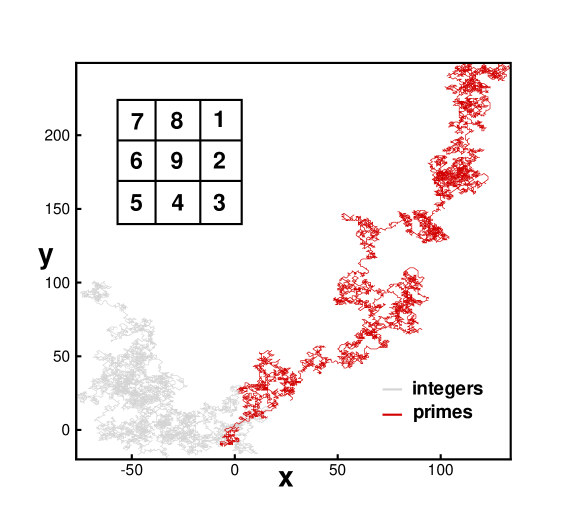
Figure 6: Random walks. Grey: 2D Random walk in which at each step we pick at random a natural from $[1,10^{6}]$ and move forward depending on the value of its first significative digit following the rules depicted in the inner table. The behavior approximates an uncorrelated Brownian motion: integers first digit is uniformly distributed. Red: same random walk but picking at random primes in $[1,10^{6}]$: in this case the random walk is clearly biased.

where $x$ and $y$ are cartesian variables with $x(0)=y(0)=0$, and both $\xi_{x}$ and $\xi_{y}$ are discrete random variables that take values $\in\{0,-1,1\}$ depending on the first digit $d$ of the numbers randomly chosen at each time step, according to the rules depicted in figure 6. Thereby, in each iteration we peak at random a positive integer (grey random walk) or a prime (red random walk) from the interval $[1,10^{6}]$, and depending on its first significative digit $d$, the random walker moves accordingly (for instance if we peak prime $13$, we have $d=1$ and the random walker rules provide $\xi_{x}=1$ and $\xi_{y}=1$: the random walker moves up-right). We have plotted the results of this 2D Random Walk in figure 6 for random picking of integers (grey random walk) and for random picking of primes (red random walk). Note that while the grey random walk seems to be a typical uncorrelated Brownian motion (enhancing the fact that the first digit distribution of the integers is uniformly distributed), the red random walk is clearly biased: this is indeed a visual characterization of the pattern. Observe that if the interval in which we randomly peak either the integers or the primes wasn’t of the shape [$1,10^{D}$], there would be a systematic bias present in the pool and consequently both integer and prime random walks would be biased: it comes thus necessary to define the intervals under study in that way.

.1.2 Natural density

If primes were for instance Benford distributed, one should expect that if we pick a prime at random, this one should start by number 1 around $30\%$ of the time. But what does the sentence ’Pick a prime at random’ stand for? Notice that in the previous experiment (the 2D biased Random Walk) we have drawn whether integers or primes at random from the pool $[1,10^{6}]$. All over the paper, the intervals $[1,N]$ have been chosen such that $N=10^{D}$, $D\in\mathbb{N}$. This choice isn’t arbitrary, much on the contrary, it relies on the fact that whenever studying infinite integer sequences, the results strongly depend on the interval under study. For instance, everyone will agree that intuitively the set of positive integers $\mathbb{N}$ is an infinite sequence whose first digit is uniformly distributed: there exist as many naturals starting by one as naturals starting by nine. However there exist subtle difficulties at this point that come from the fact that the first digit natural density is not well defined. Since there exist infinite integers in $\mathbb{N}$ and consequently it is not straightforward to quantify the quote ’pick an integer at random’ in a way in which satisfies the laws of probability, in order to check if integers have a uniform distributed first significant digit, we have to consider finite intervals $[1,N]$. Hereafter, notice that uniformity a priori is only respected when $N=10^{D}$. For instance, if we choose the interval to be $[1,2000]$, a random drawing from this interval will be a number starting by $1$ with high probability, as there are obviously more numbers starting by one in that interval. If we increase the interval to say $[1,3000]$, then the probability of drawing a number starting by $1$ or $2$ will be larger than any other. We can easily come to the conclusion that the first digit density will oscillate repeatedly by decades as $N$ increases without reaching convergence, and it is thereby said that the set of positive integers with leading digit $d$ ($d=1,2...,9$) does not possess a natural density among the integers. Note that the same phenomenon is likely to take place for the primes (see Chris Caldwell’s The Prime Pages for an introductory discussion in natural density and Benford’s law for prime numbers and references therein).

In order to overcome this subtle point, one can: (i) choose intervals of the shape $[1,10^{D}]$, where every leading digit has equal probability a priori of being picked. According to this situation, positive integers $\mathbb{N}$ have a uniform first digit distribution, and in this sense Diaconis (1977) showed that primes do not obey Benford’s law as their first digit distribution is asymptotically uniform. Or (ii) use average and summability methods such as the Cesaro or the logarithm matrix method $\ell$ (Raimi 1976) in order to define a proper first digit density that holds in the infinite limit. Some authors have shown that in this case, both the primes and the integers are said to be weak Benford sequences (Raimi 1976, Flehinger 1966, Whitney 1972).

As we are dealing with finite subsets and in order to check if a pattern really takes place for the primes, in this work we have chosen intervals of the shape $[1,10^{D}]$ to assure that samples are unbiased and that all first digits are equiprobable a priori.

.2 Statistical methods

.2.1 Method of moments

In order to estimate the best fitting between a GBL with parameter $\alpha$ and a data set, we have employed the method-of-moments. If GBL fits the empirical data, then both distributions have the same first moments, and the following relation holds:

$$\sum_{d=1}^{9}{dP(d)}=\sum_{d=1}^{9}{dP^{e}(d)}$$ (35)

where $P(d)$ and $P^{e}(d)$ are the observed normalized frequencies and GB expected probabilities for digit $d$, respectively. Using a Newton-Raphson method and iterating equation 35 until convergence, we have calculated $\alpha$ for each sample $[1,N]$.

.2.2 Statistical tests

Typically, chi-square goodness-of-fit test has been used in association with Benford’s Law (Nigrini 2000). Our null hypothesis here is that the sequence of primes follow a GBL. The test statistic is:

$$\chi^{2}=M\sum_{d=1}^{9}{{\big{(}P(d)-P^{e}(d)\big{)}^{2}}\over{P^{e}(d)}},$$ (36)

where $M$ denotes the number of primes in $[1,N]$. Since we are computing parameter $\alpha(N)$ using the mean of the distribution, the test statistic follows a $\chi^{2}$ distribution with $9-2=7$ degrees of freedom, so the null hypothesis is rejected if $\chi^{2}>\chi^{2}_{a,7}$, where $a$ is the level of significance. The critical values for the $10\%$, $5\%$, and $1\%$ are $12.02$, $14.07$, and $18.47$ respectively. As we can see in table 3, despite the excellent visual agreement (figure 1 in the main text), the $\chi^{2}$ statistic goes up with sample size and consequently the null hypothesis can’t be rejected only for relatively small sample sizes $N<10^{9}$. As a matter of fact, chi-square statistic suffers from the excess power problem on the basis that it is size sensitive: for huge data sets, even quite small differences are statistically significant (Nigrini 2000). A second alternative is to use the standard $Z$-statistics to test significant differences. However, this test is also size dependent, and hence registers the same problems as $\chi^{2}$ for large samples. Due to this facts, Nigrini (2000) recommends for Benford analysis a distance measure test called Mean Absolute Deviation (MAD). This test computes the average of the nine absolute differences between the empirical proportions of a digit and the ones expected by the GBL. That is:

$$\textrm{MAD}={1\over 9}\sum_{d=1}^{9}{\big{|}P(d)-P^{e}(d)\big{|}}$$ (37)

This test overcomes the excess power problem of $\chi^{2}$ as long as it is not influenced by the size of the data set. While MAD lacks of cut-off level, Nigrini (2000) suggests that the guidelines for measuring conformity of the first digits to Benford Law to be: MAD between $0$ and $0.4\cdot 10^{-2}$ imply close conformity, from $0.4\cdot 10^{-2}$ to $0.8\cdot 10^{-2}$ acceptable conformity, from $0.8\cdot 10^{-2}$ to $0.12\cdot 10^{-1}$ marginally acceptable conformity, and finally, greater than $0.12\cdot 10^{-1}$, nonconformity. Under these cut-off levels we can not reject the hypothesis that the first digit frequency of the prime numbers sequence follows a GBL. In addition, the Maximum Absolute Deviation $m$ defined as the largest term of MAD is also showed in each case.

As a final approach to testing for a similarity between the two histograms, we can check the correlation between the empirical and theoretical proportions by the simple regression correlation coefficient $r$ in a scatterplot. As we can see in table 3 the empirical data are highly correlated with a Generalized Benford distribution.

The same statistical tests have been performed for the case of the Riemann non trivial zeta zeros sequence (table 4), with similar results.

$N$	$M$ = # primes	$\chi^{2}$	$m$	MAD	$r$
$10^{4}$	$1229$	$0.45$	$0.32\cdot 10^{-2}$	$0.19\cdot 10^{-2}$	$0.96965$
$10^{5}$	$9592$	$0.62$	$0.21\cdot 10^{-2}$	$0.65\cdot 10^{-3}$	$0.99053$
$10^{6}$	$78498$	$0.61$	$0.50\cdot 10^{-3}$	$0.26\cdot 10^{-3}$	$0.99826$
$10^{7}$	$664579$	$0.77$	$0.17\cdot 10^{-3}$	$0.11\cdot 10^{-3}$	$0.99964$
$10^{8}$	$5761455$	$2.2$	$0.15\cdot 10^{-3}$	$0.56\cdot 10^{-4}$	$0.99984$
$10^{9}$	$50847534$	$11.0$	$0.11\cdot 10^{-3}$	$0.42\cdot 10^{-4}$	$0.99988$
$10^{10}$	$455052511$	$61.2$	$0.90\cdot 10^{-4}$	$0.33\cdot 10^{-4}$	$0.99991$
$10^{11}$	$4118054813$	$358.5$	$0.74\cdot 10^{-4}$	$0.27\cdot 10^{-4}$	$0.99993$

Table 3: Table gathering the values of the following statistics: $\chi^{2}$, Maximum Absolute Deviation ($m$), Mean Absolute Deviation (MAD) and correlation coefficient ($r$) between the observed first significant digit frequency of the set of $M$ primes in $[1,N]$ and the expected Generalized Benford distribution (eq. 2) with an exponent $\alpha(N)$ given by eq. 3 with $a=1.1$). While $\chi^{2}$-test rejects the hypothesis for very large samples due to its size sensitivity, every other test cannot reject it, enhancing the goodness-of-fit between the data and the GB distribution.

$N$	$M$ = # zeros	$\chi^{2}$	$m$	MAD	$r$
$10^{3}$	$649$	$0.14$	$0.32\cdot 10^{-2}$	$0.13\cdot 10^{-2}$	$0.99701$
$10^{4}$	$10142$	$0.23$	$0.11\cdot 10^{-2}$	$0.41\cdot 10^{-3}$	$0.99943$
$10^{5}$	$138069$	$0.75$	$0.54\cdot 10^{-3}$	$0.20\cdot 10^{-3}$	$0.99974$
$10^{6}$	$1747146$	$3.6$	$0.34\cdot 10^{-3}$	$0.13\cdot 10^{-3}$	$0.99983$
$10^{7}$	$21136126$	$20.3$	$0.23\cdot 10^{-3}$	$0.86\cdot 10^{-4}$	$0.99988$

Table 4: Table gathering the values of the following statistics: $\chi^{2}$, Maximum Absolute Deviation ($m$), Mean Absolute Deviation (MAD) and correlation coefficient ($r$) between the observed first significant digit frequency in the $M$ zeros in $[0,N]$ and the expected Generalized Benford distribution (eq. 5 with and exponent $\alpha(N)$ given by eq. 3 with $a=2.92$). While $\chi^{2}$-test rejects the hypothesis for very large samples due to its size sensitivity, every other test can’t reject it, enhancing the goodness-of-fit between the data and the GB distribution.

.3 Cramér’s model

The prime number distribution is deterministic in the sense that primes are determined by precise arithmetic rules. However, its apparent local randomness has suggested several stochastic interpretations. Concretely, Cramér (1935, see also Tenembaum 2000) defined the following model: assume that we have a sequence of urns $U(n)$ where $n=1,2,...$ and put black and white balls in each urn such that the probability of drawing a white ball in the $k^{th}$-urn goes like $1/\log k$. Then, in order to generate a sequence of pseudo-random prime numbers we only need to draw a ball from each urn: if the drawing from the $k^{th}$-urn is white, then $k$ will be labeled as a pseudo-random prime. The prime number sequence can indeed be understood as a concrete realization of this stochastic process. With such model, Cramér studied amongst others the distribution of gaps between primes and the distribution of twin primes as far as statistically speaking, these distributions should be similar to the pseudo-random ones generated by his model. Quoting Cramér: ‘With respect to the ordinary prime numbers, it is well known that, roughly speaking, we may say that the chance that a given integer $n$ should be a prime is approximately $1/\log n$. This suggests that by considering the following series of independent trials we should obtain sequences of integers presenting a certain analogy with the sequence of ordinary prime numbers $p_{n}$’.

In this work we have simulated a Cramér process, in order to obtain a sample of pseudo-random primes in $[1,10^{11}]$. Then, the same statistics performed for the prime number sequence have been realized in this sample. Results are summarized in table 5. We can observe that the Cramér’s model reproduces the same behavior, namely: (i) The first digit distribution of the pseudo-random prime sequence follows a GBL with a size-dependent exponent that follows eq. 3. (ii) The number of pseudo-primes found in each decade matches statistically speaking to the actual number of primes. (iii) The $\chi^{2}$-test evidences the same problems of power for large data sets. Having in mind that the sample elements in this model are independent (what is not the case in the actual prime sequence), we can confirm that the rejection of the null hypothesis by the $\chi^{2}$-test for huge data sets is not related to a lack of data independence but much likely to the test’s size sensitivity. (iv) The rest of statistical analysis is similar to the one previously performed in the prime number sequence.

$N$	$M$ = # pseudo-random primes	$\chi^{2}$	$m$	MAD	$r$
$10^{4}$	$1189$	$1.20$	$0.17\cdot 10^{-1}$	$0.92\cdot 10^{-2}$	$0.639577$
$10^{5}$	$9673$	$0.43$	$0.33\cdot 10^{-2}$	$0.21\cdot 10^{-2}$	$0.969031$
$10^{6}$	$78693$	$0.39$	$0.59\cdot 10^{-3}$	$0.14\cdot 10^{-2}$	$0.990322$
$10^{7}$	$664894$	$0.09$	$0.23\cdot 10^{-3}$	$0.99\cdot 10^{-4}$	$0.999626$
$10^{8}$	$5762288$	$0.24$	$0.15\cdot 10^{-3}$	$0.53\cdot 10^{-4}$	$0.999855$
$10^{9}$	$50850064$	$1.23$	$0.11\cdot 10^{-3}$	$0.42\cdot 10^{-4}$	$0.999892$
$10^{10}$	$455062569$	$6.84$	$0.90\cdot 10^{-4}$	$0.33\cdot 10^{-4}$	$0.999914$
$10^{11}$	$4118136330$	$41.0$	$0.73\cdot 10^{-4}$	$0.27\cdot 10^{-4}$	$0.999937$

Table 5: Table gathering the values of the following statistics: $\chi^{2}$, Maximum Absolute Deviation ($m$), Mean Absolute Deviation (MAD) and correlation coefficient ($r$) between the observed first significant digit frequency in the Cramér model for $M$ pseudo-random primes in $[1,N]$ and the expected Generalized Benford distribution (eq. 2 with an exponent $\alpha(N)$ given by eq. 3 with $a=1.1$).

Figure 3: Extension of GBL to the $k$ first significant digits. In this figure we represent the fitting of an extended GBL following eq. 4 (black line) to the first two significant digits relative frequencies (up-left), first three significant digits relative frequencies (up-right), first four significant digits relative frequencies (down-left) and first five significant digits relative frequencies (down-right) of the $4118054813$ primes appearing in the interval $[1,10^{11}]$ (red dots).

Figure 5: Extension of GBL to the $k$ first significant digits. In this figure we represent the fitting of an extended GBL following eq. 6 (black line) to the first two significant digits relative frequencies (up), first three significant digits relative frequencies (down-left), and first four significant digits relative frequencies (down-right) of the $21136126$ zeros appearing in the interval $[1,10^{7}]$ (blue dots).