Variational approach to the scaling function of the 2D Ising model in a magnetic field

Abstract

The universal scaling function of the square lattice Ising model in a magnetic field is obtained numerically via Baxter’s variational corner transfer matrix approach. The high precision numerical data is in perfect agreement with the remarkable field theory results obtained by Fonseca and Zamolodchikov, as well as with many previously known exact and numerical results for the 2D Ising model. This includes excellent agreement with analytic results for the magnetic susceptibility obtained by Orrick, Nickel, Guttmann and Perk. In general the high precision of the numerical results underlines the potential and full power of the variational corner transfer matrix approach.

^aDepartment of Theoretical Physics,
Research School of Physics and Engineering,
^bMathematical Sciences Institute,
Australian National University, Canberra, ACT 0200, Australia.

The Ising model has played a prominent role in the development of the theory of phase transition and critical phenomena [1, 2, 3, 4, 5, 6, 7, 8]. The partition function of the nearest-neighbour Ising model on the square lattice reads

$${Z}=\sum_{\sigma}\exp\Big{\{}\,\beta\sum_{\langle ij\rangle}\sigma_{i}\sigma_{j}+{H}\sum_{i}\sigma_{i}\,\Big{\}}\ ,\qquad\sigma_{i}=\pm 1,$$ (1)

where the first sum in the exponent is taken over all edges, the second over all sites and the outer sum over all spin configurations $\{\sigma\}$ of the lattice. The constants $H$ and $\beta$ denote the (suitably normalized) magnetic field and inverse temperature. The specific free energy, magnetization and magnetic susceptibility are defined as

$$F=-\lim_{N\to\infty}\frac{1}{N}\log Z,\qquad M=-\frac{\partial F}{\partial H},\qquad\chi=-\frac{\partial^{2}F}{\partial H^{2}}\ ,$$ (2)

where $N$ is the number of lattice sites. The model exhibits a second order phase transition at $\beta=\beta_{c}$, $H=0$, where [1]

$$\beta_{c}=\frac{1}{2}\log(1+\sqrt{2})=0.44068679\ldots\ .$$ (3)

In what follows we will exclude the temperature variable $\beta$ in favour of a new variable

$$2\tau={\rm cosech}(2\beta)-\sinh(2\beta)\ ,\qquad\tau_{c}=0,$$ (4)

which is vanishing for $\beta=\beta_{c}$ and positive for $\beta<\beta_{c}$ (above the critical temperature). Note also that this variable changes sign under the Kramers-Wannier duality transformation for $H=0$. Another useful related variable is

$$k=k(\tau)=(\sqrt{1+\tau^{2}}+\tau)^{2}.$$ (5)

According to the scaling theory [9, 10, 6], the leading singular part, $F_{sing}(\tau,H)$, of the free energy (2) in the vicinity of the critical point can be expressed through a universal function ${\mathcal{F}}(m,h)$,

$$F_{sing}(\tau,H)={\mathcal{F}}(m(\tau,H),h(\tau,H)),\qquad\tau\to 0,\quad H\to 0,$$ (6)

where $\tau$ and $H$ enter the RHS only through non-linear scaling variables [11],

$$m=m(\tau,H)=-\sqrt{2}\,\tau+O(\tau^{3})+O(H^{2})+\ldots,\quad h=h(\tau,H)=C_{h}\,H+H\,O(\tau)+O(H^{3})\ldots,\qquad$$ (7)

which are analytic functions of $\tau$ and $H$. The coefficients in these expansions (for instance, the leading coefficients $-\sqrt{2}$ and $C_{h}$) are specific to the square lattice Ising model, however, the function ${\mathcal{F}}(m,h)$ is the same for all models in the 2D Ising model universality class. It can be written as

$${\mathcal{F}}(m,h)=\frac{m^{2}}{8\pi}\,\log m^{2}+h^{16/15}\,\Phi(\eta),\qquad\eta=\frac{m}{h^{8/15}}$$ (8)

where $\Phi(\eta)$ is a universal scaling function of a single variable $\eta$ (the scaling parameter).

The function ${\mathcal{F}}(m,h)$ has a concise interpretation in terms of 2D Euclidean quantum field theory. Namely, it coincides with the vacuum energy density of the “Ising Field Theory” (IFT) [12]. The latter is defined as a model of perturbed conformal field theory with the action

$${\cal A}_{\rm IFT}={\cal A}_{(c=1/2)}+\frac{m}{2\pi}\,\int\,\epsilon(x)\,d^{2}x+h\,\int\,\sigma(x)\,d^{2}x\,,$$ (9)

where ${\cal A}_{(c=1/2)}$ stands for the action of the $c=1/2$ CFT of free massless Majorana fermions, $\sigma(x)$ and $\epsilon(x)$ are primary fields of conformal dimensions $1/16$ and $1/2$. Their normalization is fixed by the usual CFT convention,

$$|x|^{2}\,\langle\epsilon(x)\epsilon(0)\rangle\to 1\,;\qquad|x|^{1/4}\,\langle\sigma(x)\sigma(0)\rangle\to 1\,\quad{\rm as}\quad|x|\to 0\,.$$ (10)

With this normalization, the parameters $m$ and $h$ have the mass dimensions $1$ and $15/8$, respectively, and the scaling parameter $\eta$ in (8) is dimensionless.

The scaling function (8) is of much interest as it controls all thermodynamic properties of the Ising model in the critical domain. Although there are many exact results (obtained through exact solutions of (9) at $h=0$ and all $\tau$ [1, 13, 3, 14, 15, 16], and at $\tau=0$ and all $h$ [8, 17, 18, 19, 20, 21, 22]; these data are collected in [23]) as well as much numerical data [24, 25, 26, 27, 28] about this function, its complete analytic characterization is still lacking.

Recently [12] the function (8), particularly its analytic properties, have been thoroughly studied in the framework of the Ising Field Theory (9). The authors of [12] made extensive numerical calculations of the scaling function $\Phi(\eta)$ using the “Truncated Free-Fermion Space Approach” (TFFSA), which is a modification of the well-known “Truncated Conformal Space Approach” (TCSA)[29, 30].

The primary motivation of our work was to confirm and extend the field theory results of ref. [12] through ab initio calculations, directly from the original lattice formulation (1) of the Ising model. We used Baxter’s variational approach based on the corner transfer matrix method [31, 32, 33]. The main advantage of this approach over other numerical schemes (e.g., the row-to-row transfer matrix method) is that it is formulated directly in the limit of an infinite lattice. Its accuracy depends on the magnitude of truncated eigenvalues of the corner transfer matrix (which is at our control), rather than the size of the lattice. The details of our calculations along with numerical data for the free energy, magnetization and internal energy of the Ising model will be presented elsewhere [34]. We used several important enhancements of the original Baxter approach [32], in particular an improved iteration scheme [35], known as the corner transfer matrix renormalization group (CTMRG). The calculations were performed for a grid of values of the magnetic field and temperature in the range $10^{-7}<H<10^{-2}$ and $0.9\beta_{c}<\beta<1.1\beta_{c}$, containing about $10,000$ distinct point (excluding a small region around the critical point). The results for the scaling function $\Phi(\eta)$ are shown in Fig. 1. All calculated data points collapse on a smooth curve, shown by the solid line (additional details presented on the picture are explained below). Our numerical results for $\Phi(\eta)$ remarkably confirm the field theory calculations of [12], to within all six significant digits presented therein.

The precision of our numerical calculations was tested against all available exact results for the Ising model. In particular, the agreement between calculated and exact values for the zero-field free energy [1], magnetization [2] and magnetic susceptibility [36] in our working range of temperatures varied between 14 and 28 decimal places (depending on the distance to the critical point). In addition to these checks we also confirmed and extended many previously existing numerical results for the Ising model. Some details of our results are described below.

For the following discussion it is convenient to rewrite (8) in an alternative form, introducing two more scaling functions,

$${\mathcal{F}}(m,h)=\frac{m^{2}}{8\pi}\,\log m^{2}+\left\{\begin{array}[]{ll}m^{2}\,G_{high}(\xi),&\quad m<0\\ m^{2}\,G_{low}(\xi),&\quad m>0\end{array}\right.\ ,\qquad\xi={h}/{|m|^{15/8}}\ .$$ (11)

where $G_{high}(0)=G_{low}(0)=0$, corresponding to

$${\mathcal{F}}(m,0)=\frac{m^{2}}{8\pi}\,\log m^{2}\ .$$ (12)

These scaling functions are thoroughly discussed in [12]. The function $G_{high}(\xi)$ can be expanded in a series in even powers of $\xi$

$$G_{high}(\xi)=G_{2}\xi^{2}+G_{4}\xi^{4}+G_{6}\xi^{6}+\ldots$$ (13)

convergent in some domain around the origin of the $\xi$-plane. The function $G_{low}(\xi)$ admits an asymptotic expansion

$$G_{low}(\xi)=\tilde{G}_{1}\xi+\tilde{G}_{2}\xi^{2}+\tilde{G}_{3}\xi^{3}+\ldots$$ (14)

for small positive $\xi$. These new functions are simply related to $\Phi(\eta)$. Note, in particular, that the coefficients $G_{n}$ and $\tilde{G}_{n}$ control the behavior of the function $\Phi(\eta)$ for large values of $\eta$ on the real line,

$$\Phi_{low}(\eta) = \tilde{G}_{1}\eta^{\frac{1}{8}}+\tilde{G}_{2}\eta^{-\frac{7}{4}}+\tilde{G}_{3}\eta^{-\frac{29}{8}}+\ldots\,\qquad\qquad\qquad{\rm for\ real}\quad\eta\to+\infty\,,$$ (15)

$$\Phi_{high}(\eta) = G_{2}(-\eta)^{-\frac{7}{4}}+G_{4}(-\eta)^{-\frac{22}{4}}+G_{6}(-\eta)^{-\frac{37}{4}}+\ldots\quad{\rm for\ real}\quad\eta\to-\infty\,.$$ (16)

Finally, for small values of $\eta$,

$$\Phi(\eta)=-{\frac{\eta^{2}}{8\pi}}\,\log\eta^{2}+\sum_{k=0}^{\infty}\Phi_{k}\eta^{k}$$ (17)

where the series converges in a finite domain around the origin of the complex $\eta$-plane.

Some of the above expansion coefficients are known exactly. The coefficient $\tilde{G}_{1}$ is known explicitly [4]

$$\tilde{G}_{1}=-2^{1/12}\,e^{-1/8}\,{\mathcal{A}}^{3/2}=-1.357838341706595\ldots\ ,$$ (18)

where ${\mathcal{A}}=1.282427\ldots$ is the Glaisher constant. The coefficients $G_{2}$ and $\tilde{G}_{2}$ have integral expressions [14, 15] involving solutions of the Painlevé III equation. They were numerically evaluated to very high precision (50 digits) in [36],

$$G_{2}=-1.845228078232838\ldots,\qquad\tilde{G}_{2}=-0.0489532897203\ldots\ .$$ (19)

The coefficient $\Phi_{0}$ was calculated in [17],

$$\Phi_{0}=-\frac{(2\pi)^{\frac{1}{15}}\gamma(\frac{1}{3})\gamma(\frac{1}{5})\gamma(\frac{7}{15})}{\left[\gamma(\frac{1}{4})\gamma^{2}(\frac{3}{16})\right]^{\frac{8}{15}}}=-1.19773338379799\ldots,\qquad\gamma(x)=\frac{\Gamma(x)}{\Gamma(1-x)}$$ (20)

where $\Gamma(x)$ is the standard $\Gamma$-function. The coefficient $\Phi_{1}$ has an explicit integral representation, obtained in [37]. We have evaluated the required integral explicitly,

$$\Phi_{1}=-\frac{32\cdot 2^{\frac{3}{4}}}{225\>(2\pi)^{\frac{7}{15}}}\frac{\gamma(\frac{1}{3})\gamma(\frac{1}{8})\prod\limits_{k=3}^{7}\gamma(\frac{k}{15})}{\left[\gamma(\frac{1}{4})\gamma^{2}(\frac{3}{16})\right]^{\frac{19}{15}}}=-0.3188101248906\ldots\ .$$ (21)

Contrary to the field theory case, the lattice free energy,

$$F(\tau,H)=F_{sing}(\tau,H)+F_{reg}(\tau,H)+F_{sub}(\tau,H),\qquad\tau,H\to 0,$$ (22)

never coincides with its leading universal part (6). It also contains regular terms $F_{reg}(\tau,H)$, analytic in $\tau$ and $H$, as well as subleading singular terms $F_{sub}(\tau,H)$, which are non-analytic, but less singular than the first term in (22). Therefore, to extract the universal scaling function from the lattice calculations one should be able to isolate and subtract these extra terms. Moreover, one needs to know the explicit form of the non-linear scaling variables (7). In principle, all this information can be determined entirely from numerical calculations (provided one assumes the values of exponents of the subleading terms, predicted by the analysis [38, 36] of the CFT irrelevant operators, contributing to the free energy (22)). The accuracy of this “fully numerical” approach, however, deteriorates rapidly for the higher order terms. Much more accurate results can be obtained if the numerical work is combined with known exact results.

Write the non-linear variables (7) in the form,

$$m(\tau,H) = -\sqrt{2}\,\tau\ a(\tau)+H^{2}\,b(\tau)+O(H^{4})\ ,$$

$$h(\tau,H) = C_{h}H\,\Big{[}c(\tau)+H^{2}\,d(\tau)+O(H^{4})\Big{]}\ ,$$ (23)

where $a(0)=c(0)=1$, $h(\tau,H)=-h(\tau,-H)$. Similarly, write the regular part as,

$$F_{reg}(\tau,H)=A(\tau)+H^{2}\,B(\tau)+O(H^{4})\ .$$ (24)

As shown in [36], the most singular subleading term, contributing to (22) is of the order of $O(\tau^{9/4}\,H^{2})$ (see Eq.(36) below). The fact that subleading terms arise only in such a high order ($\sim m^{6}$) is a remarkable property of the square lattice nearest-neighbour Ising model, which greatly simplifies the calculation of the universal scaling function from the numerical data.

For $H=0$ the expression (22) should reduce to Onsager’s exact result [1]

$$F(\tau,0)=\log\sqrt{2}\cosh(2\beta)+\int_{0}^{\pi}\frac{d\theta}{2\pi}\,\log\Big{[}1+\Big{(}1-\frac{\cos^{2}\theta}{1+\tau^{2}}\Big{)}^{1/2}\Big{]}\ .$$ (25)

Therefore one should be able to rewrite the last formula in the form (12) plus regular terms. This is achieved by choosing [39]

$$a(\tau)=\left[\int_{0}^{1}dx\,F({\textstyle\frac{1}{2}},{\textstyle\frac{1}{2}},1;-x\tau^{2})/(1+x\tau^{2})^{1/2}\right]^{1/2}={1-\frac{3\tau^{2}}{16}+\frac{137\tau^{4}}{1536}+O(\tau^{6})}\ ,$$ (26)

where $F(a,b,c,z)$ denotes the Gauss hypergeometric function. The corresponding contribution to (24) then reads

$$A(\tau)=-\frac{\displaystyle 2{\mathcal{G}}}{\displaystyle\pi}-\frac{\displaystyle\log 2}{\displaystyle 2}+\frac{\displaystyle\tau}{\displaystyle 2}-\frac{\displaystyle\tau^{2}(1+5\log 2)}{\displaystyle 4\pi}-\frac{\displaystyle\tau^{3}}{\displaystyle 12}+\frac{\displaystyle 5\tau^{4}(1+6\log{2})}{\displaystyle 64\pi}+O(\tau^{5})\ ,$$ (27)

where ${\mathcal{G}}=0.915965594\ldots$ is the Catalan constant.

Next, using the exact expression for the zero field magnetization [2, 3]

$$M(\tau,0)=(1-k(\tau)^{2})^{1/8},\qquad\tau<0$$ (28)

with $k(\tau)$ defined in (5), one finds from (1), (11), (14) and (22)

$$c(\tau)=\frac{M(\tau)}{(-4\tau\,a(\tau))^{1/8}}=1+\frac{\tau}{4}+\frac{15\tau^{2}}{128}-\frac{9\tau^{3}}{512}-\frac{4333\tau^{4}}{98304}+O(\tau^{5})\ ,$$ (29)

and also

$$C_{h}=-2^{3/16}/\tilde{G}_{1}=0.838677624411\ldots\ .$$ (30)

Finally, consider the zero-field susceptibility. No simple closed form expression for the zero-field susceptibility $\chi(\tau)$ is known. However, the authors of [36] obtained remarkable asymptotic expansions of $\chi(\tau)$ for small $\tau$ to within $O(\tau^{14})$ terms with high-precision numerical coefficients. We have compared their series with our numerical results for the susceptibility in the range of temperatures $|\tau|=0.05\mbox{--}0.14$ and found that they agree to each other in 14 to 18 significant digits (depending on the value of $\tau$). Their result can be written as (retaining the terms up to $O\big{(}|\tau|^{9/4}\big{)}$, inclusive)

$$\chi(\tau)_{\rm ONGP} = -2^{-\frac{7}{8}}\,C_{h}^{2}\,G^{\prime\prime}(0)\ |\tau|^{-\frac{7}{4}}\Big{(}1+\frac{\tau}{2}+\frac{5\tau^{2}}{8}+\frac{3\tau^{3}}{16}-\frac{23\tau^{4}}{384}+O(\tau^{5})\Big{)}$$ (31)

$$+e(\tau)+f(\tau)\log|\tau|+O(\tau^{3}\log|\tau|)$$

where $e(\tau)$ and $f(\tau)$ are explicitly known second order polynomials in $\tau$. The coefficient in front of the first term is written in our notations. The symbol $G^{\prime\prime}(0)$ there stands for the second derivative of the scaling function $G(\xi)$ with respect to its argument. Namely $G^{\prime\prime}(0)=G_{high}^{\prime\prime}(0)=2G_{2}$ for $\tau>0$ and $G^{\prime\prime}(0)=G_{low}^{\prime\prime}(0)=2\tilde{G}_{2}$ for $\tau<0$. The corresponding values are given in (19) above. Next, calculating the second field derivative of (22) at $H=0$, one obtains

$$\chi(\tau) = -2^{-\frac{7}{8}}\,C_{h}^{2}\,G^{\prime\prime}(0)\ |\tau|^{-\frac{7}{4}}\,a(\tau)^{-\frac{7}{4}}\,c(\tau)^{2}-\frac{\partial^{2}F_{sub}(\tau,H)}{\partial H^{2}}\Big{|}_{H=0}$$ (32)

$$-2B(\tau)+\frac{\tau\,a(\tau)\,b(\tau)}{\sqrt{2}\,\pi}\Big{(}1+\log\big{(}2\tau^{2}a(\tau)\big{)}\Big{)}\ .$$

Equating this expression to (31) and using (26), (29) and explicit forms of the polynomials $e(\tau)$ and $f(\tau)$ from [36], one obtains

$$B(\tau)=0.0520666225469+0.0769120341893\,\tau+0.0360200462309\,\tau^{2}+O(\tau^{3})\ ,$$ (33)

and

$$b(\tau)=\mu_{h}\,\Big{(}1+\frac{\tau}{2}+O(\tau^{2})\Big{)},\qquad\mu_{h}=0.071868670814\ .$$ (34)

Noting that

$$a(\tau)^{-\frac{7}{4}}\,c(\tau)^{2}=1+\frac{\tau}{2}+\frac{5\tau^{2}}{8}+\frac{3\tau^{3}}{16}-\frac{11\tau^{4}}{192}+O(\tau^{5})$$ (35)

one immediately obtains the main contribution to the subleading term

$$\Big{(}2^{-\frac{7}{8}}\,C_{h}^{2}\,G^{\prime\prime}(0)\Big{)}^{-1}\,\frac{\partial^{2}F_{sub}(\tau,H)}{\partial H^{2}}\Big{|}_{H=0}=-\frac{1}{384}\,\,|\tau|^{\frac{9}{4}}+\ldots\ .$$ (36)

The results of [36] provided the first convincing demonstration of the violation to simple one-parametric scaling in the square lattice Ising model. Note that despite the $O(|\tau|^{9/4})$ term gives a very small contribution to the susceptibility we were able to confidently quantify it from our numerical results. Namely, we estimated the coefficient of the $\tau^{4}$ term in the series shown in parenthesis in the first line of (31). Our estimate is $23.004/384$ which is within $0.02\%$ of its exact value $23/384$.

The coefficient $d(\tau)$ in (23) was estimated from our numerical data for the internal energy,

$$d(\tau)=e_{h}+O(\tau),\qquad e_{h}=-0.007(1),$$ (37)

which is in agreement with the result $e_{h}=-0.00727(15)$ from [26].

The above expressions were used to analyze our extensive numerical data and extract the necessary information to obtain the universal scaling function. The results are summarized in four tables. For convenience of comparison we quoted the corresponding results from [12], including those obtained through the TFFSA, the high/low-temperature and extended dispersion relations (DR). Earlier exact and numerical results for the same quantities are also quoted (whenever available). Figure 1 shows about 10,000 data points for the scaling function $\Phi(\eta)$. As expected, the points collapse on a smooth curve (their spread is much smaller than the resolution of the picture). Figure 1 also shows plots of the asymptotic expansions (15), (16) and (17) with the coefficients given in Table 1, Table 2 and Table 3. These expansions are seen to “stitch” together very well and give a reasonably good analytic approximation to $\Phi(\eta)$ in the whole real line of $\eta$. Our Fig. 1 essentially coincides with Fig. 10 of [12]. The numerical values of $\Phi(\eta)$ at small integer values of $\eta$ are given in Table 4.

The calculations were performed on the 24-processor Linux Cluster System at the ANU Research School of Physics and Engineering and on the 1928-processor SGI Altix 3700 Bx2 Cluster at the ANU Supercomputer Facility. The level of parallelization varied between 15 and 50 processors. The total amount of CPU time spent for this work was about 9,000 hours (single processor equivalent).

To conclude, we have implemented Baxter’s variational corner transfer matrix approach to obtain the universal scaling function of the square lattice Ising model in a magnetic field, as shown in Figure 1 and Table 4. The numerical data is seen to be in remarkable agreement with the field theory results obtained by Fonseca and Zamolodchikov [12]. We also report a remarkable agreement (11 to 14 digits) between our numerical values for $\tilde{G}_{1}$, $G_{2}$ and $\tilde{G}_{2}$ and the classic exact results of Barouch, McCoy, Tracy and Wu [4, 14, 15] (see Tables 1 and 2), and a similar agreement between the values $\Phi_{0}$ and $\Phi_{1}$ and the exact predictions [17, 37] of Zamolodchikov’s integrable $E_{8}$ field theory [8] (see Table 3). The high precision of the numerical results underline the full power and further potential of the variational corner transfer matrix approach. In this case, the results show beyond any doubt the validity of the connection between the scaling limit of the Ising model in a magnetic field and the Ising Field Theory (9).

The authors thank H. Au-Yang, R.J. Baxter, G. Delfino, S.L. Lukyanov, J.H.H. Perk, C.A. Tracy and A.B. Zamolodchikov for useful discussions and remarks. This work has been partially supported by the Australian Research Council.

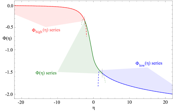
Figure 1: Scaling function of the two-dimensional Ising model in a magnetic field. The figure shows about 10,000 data points for the scaling function $\Phi(\eta)$. As expected, the points collapse on a smooth curve (their spread is much smaller than the resolution of the picture). The figure also shows plots of the asymptotic expansions (15), (16) and (17) with the coefficients given in Table 1, Table 2 and Table 3.

	CTM (This work)	High-$T$ DR [12]	From References
$G_{2}$	$-1.8452280782328(2)$	$-1.8452283$	$-1.845228078232838...$	[14, 15, 36]
$G_{4}$	$\phantom{+}8.333711750(5)$	$\phantom{+}8.33410$	$\phantom{+}8.33370(1)$	[26]
$G_{6}$	$-95.16896(1)$	$-95.1884$	$-95.1689(4)$	[26]
$G_{8}$	$\phantom{+}1457.62(3)$	$\phantom{+}1458.21$	$\phantom{+}1457.55(11)$	[26]
$G_{10}$	$-25891(2)$	$-25889$	$-25884(13)$	[26]

Table 1: Numerical values of the coefficients $G_{2n}$ in (13). The second column contains the high-temperature dispersion relation (DR) results from [12]. The coefficient $G_{2}$ is known exactly [14, 15, 36].

	CTM (This work)	Low-$T$ DR [12]	From References
$\tilde{G}_{1}$	$-1.3578383417066(1)$	$-1.35783835$	$-1.357838341706595...$ [4]
$\tilde{G}_{2}$	$-0.048953289720(1)$	$-0.0489589$	$-0.0489532897203...$ [14, 15, 36]
$\tilde{G}_{3}$	$\phantom{+}0.038863932(3)$	$\phantom{+}0.0388954$	$\phantom{+}0.0387529$ [40]; $\phantom{+}0.039(1)$ [25]
$\tilde{G}_{4}$	$-0.068362119(2)$	$-0.0685060$	$-0.0685535$ [40]; $-0.0685(2)$ [25]
$\tilde{G}_{5}$	$\phantom{+}0.18388370(1)$	$\phantom{+}0.18453$	—
$\tilde{G}_{6}$	$-0.6591714(1)$	$-0.66215$	—
$\tilde{G}_{7}$	$\phantom{+}2.937665(3)$	$\phantom{+}2.952$	—
$\tilde{G}_{8}$	$-15.61(1)$	$-15.69$	—

Table 2: Numerical values of the coefficients $\tilde{G}_{n}$ in (14). The second column contains the low-temperature dispersion relation results from [12]. The right column refers to exact values of $\tilde{G}_{1}$ [4] and $\tilde{G}_{2}$ [14, 15, 36] and other numerical results.

	CTM (This work)	TFFSA [12]	Ext. DR [12]	From References
$\Phi_{0}$	$-1.197733383797993(1)$	$-1.1977331$	$-1.1977320$	$-1.19773338379799339...$ [17]
$\Phi_{1}$	$-0.318810124891(1)$	$-0.3188103$	$-0.3188192$	$-0.3188101248906...$ [37]
$\Phi_{2}$	$\phantom{+}0.110886196683(2)$	$\phantom{+}0.1108867$	$\phantom{+}0.1108915$	—
$\Phi_{3}$	$\phantom{+}0.01642689465(2)$	$\phantom{+}0.0164266$	$\phantom{+}0.0164252$	—
$\Phi_{4}$	$-2.639978(1)\times 10^{-4}$	$-2.64\times 10^{-4}$	$-2.64\times 10^{-4}$	—
$\Phi_{5}$	$-5.140526(1)\times 10^{-4}$	$-5.14\times 10^{-4}$	$-5.14\times 10^{-4}$	—
$\Phi_{6}$	$\phantom{+}2.08865(1)\times 10^{-4}$	$\phantom{+}2.07\times 10^{-4}$	$\phantom{+}2.09\times 10^{-4}$	—
$\Phi_{7}$	$-4.4819(1)\times 10^{-5}$	$-4.52\times 10^{-5}$	$-4.48\times 10^{-5}$	—
$\Phi_{8}$	—	—	$\phantom{+}3.16\times 10^{-7}$	—
$\Phi_{9}$	—	—	$\phantom{+}4.31\times 10^{-6}$	—
$\Phi_{10}$	—	—	$-1.99\times 10^{-6}$	—

Table 3: Numerical values of the coefficients $\Phi_{n}$ in (17). The second and third columns contain results from [12], obtained through the TFFSA and the extended dispersion relations (DR), respectively. The forth column refers to exact results; the numerical value of $\Phi_{1}$ therein is taken from Eq.(21).

$\Phi(\eta)$	CTM (This work)	TFFSA [12]	High/Low-$T$ DR [12]	Ext. DR [12]
$\Phi(-5)$	$-0.10920919$	$-0.1092101$	$-0.1092092$	$-0.1088626$
$\Phi(-4)$	$-0.15926438$	$-0.1592682$	$-0.1592643$	$-0.1589421$
$\Phi(-3)$	$-0.25298908$	$-0.2529928$	$-0.2529887$	$-0.2527417$
$\Phi(-2)$	$-0.44132564$	$-0.4413450$	$-0.4413249$	$-0.4412136$
$\Phi(-1)$	$-0.78396650$	$-0.7839665$	$-0.7839668$	$-0.7839576$
$\Phi(0)$	$-1.19773338$	$-1.1977330$	—	$-1.1977320$
$\Phi(1)$	$-1.38984135$	$-1.3898410$	$-1.3898417$	$-1.3898063$
$\Phi(2)$	$-1.49305602$	$-1.4930558$	$-1.4930566$	$-1.4929849$
$\Phi(3)$	$-1.56427320$	$-1.5642732$	$-1.5642736$	$-1.5641727$
$\Phi(4)$	$-1.61885066$	$-1.6188506$	$-1.6188510$	$-1.6187275$
$\Phi(5)$	$-1.66324828$	$-1.6632483$	$-1.6632485$	$-1.6631076$

Table 4: Numerical values of $\Phi(\eta)$ at small integer values of $\eta$. The second, third and fourth columns contain results [12] from the TFFSA, the high/low-temperature dispersion and the extended dispersion relations (DR).

References

- [1] Onsager, L. Crystal statistics. I. A two-dimensional model with an order-disorder transition. Phys. Rev. (2) 65 (1944) 117–149.
- [2] Onsager, L. Discussion remark (Spontaneous magnetisation of the two-dimensional Ising model). Nuovo Cimento (Suppl.) 6 (1949) 261.
- [3] Yang, C. N. The spontaneous magnetization of a two-dimensional Ising model. Phys. Rev. 85 (1952) 808.
- [4] McCoy, B. and Wu, T. T. The Two-Dimensional Ising Model. Harvard University Press, 1973.
- [5] Baxter, R. J. Exactly Solved Models in Statistical Mechanics. Academic Press Inc., London, 1982.
- [6] Aharony, A. and Fisher, M. E. Nonlinear scaling fields and corrections to scaling near criticality. Phys. Rev. B 27 (1983) 4394–4400.
- [7] Belavin, A. A., Polyakov, A. M., and Zamolodchikov, A. B. Infinite conformal symmetry in two-dimensional quantum field theory. Nucl. Phys. B 241 (1984) 333–380.
- [8] Zamolodchikov, A. B. Integrals of Motion and -matrix of the (scaled) Ising Model with Magnetic Field. Internat. J. Modern Phys. A 4 (1989) 4235–4248.
- [9] Patashinskii, A. Z. and Pokrovskii, V. L. Fluctuation theory of phase transitions. Pergamon, Oxford, 1979.
- [10] Cardy, J. Scaling and Renormalization in Statistical Physics. Cambridge University Press, 1996.
- [11] Aharony, A. and Fisher, M. E. Universality in Analytic Corrections to Scaling For Planar Ising Models. Phys. Rev. Lett. 45 (1980) 679–682.
- [12] Fonseca, P. and Zamolodchikov, A. Ising field theory in a magnetic field: analytic properties of the free energy. J. Stat. Phys. 110 (2003) 527–590. Special issue in honor of Michael E. Fisher’s 70th birthday (Piscataway, NJ, 2001).
- [13] Kaufman, B. Crystal Statistics. II. Partition Function Evaluated by Spinor Analysis. Phys. Rev. 76 (1949) 1232–1243.
- [14] Barouch, E., McCoy, B. M., and Wu, T. T. Zero-field susceptibility of the two-dimensional Ising model near . Phys. Rev. Lett. 31 (1973) 1409–1411.
- [15] Tracy, C. A. and McCoy, B. M. Neutron Scattering and the Correlation Functions of the Ising Model near . Phys. Rev. Lett. 31 (1973) 1500–1504.
- [16] Wu, T. T., McCoy, B. M., Tracy, C. A., and Barouch, E. Spin-spin correlation functions for the two-dimensional Ising model: exact theory in the scaling region. Phys. Rev. B 13 (1976) 316–374.
- [17] Fateev, V. A. The exact relations between the coupling constants and the masses of particles for the integrable perturbed conformal field theories. Phys. Lett. B 324 (1994) 45–51.
- [18] Delfino, G. and Mussardo, G. The spin-spin correlation function in the two-dimensional Ising model in a magnetic field at . Nuclear Physics B 455 (1995) 724 – 758.
- [19] Warnaar, S. O., Nienhuis, B., and Seaton, K. A. New construction of solvable lattice models including an Ising model in a field. Phys. Rev. Lett. 69 710–712.
- [20] Warnaar, S. O., Pearce, P. A., Seaton, K. A., and Nienhuis, B. Order Parameters of the Dilute A-Models. J. Stat. Phys. 74 (1994) 469–531.
- [21] Bazhanov, V. V., Nienhuis, B., and Warnaar, S. O. Lattice Ising model in a field: scattering theory. Phys. Lett. B 322 (1994) 198–206.
- [22] Batchelor, M. T. and Seaton, K. A. Magnetic correlation length and universal amplitude of the lattice Ising model. J. Phys. A 30 (1997) L479–L484.
- [23] Delfino, G. Integrable field theory and critical phenomena: the Ising model in a magnetic field. J. Phys. A 37 (2004) R45–R78.
- [24] Essam, J. W. and Hunter, D. L. Critical behaviour of the Ising model above and below the critical temperature. J. Phys. C 1 (1968) 392–407.
- [25] Zinn, S.-Y., Lai, S.-N., and Fisher, M. E. Renormalized coupling constants and related amplitude ratios for Ising systems. Phys. Rev. E 54 (1996) 1176–1182.
- [26] Caselle, M., Hasenbusch, M., Pelissetto, A., and Vicari, E. The critical equation of state of the two-dimensional Ising model. J. Phys. A 34 (2001) 2923–2948.
- [27] Caselle, M. and Hasenbusch, M. Critical amplitudes and mass spectrum of the 2d Ising model in a magnetic field. Nucl. Physics B 579 (2000) 667–703.
- [28] Caselle, M., Hasenbusch, M., Pelissetto, A., and Vicari, E. High-precision estimate of in the 2D Ising model. J. Phys. A 33 (2000) 8171–8180.
- [29] Yurov, V. P. and Zamolodchikov, Al. B. Truncated Conformal Space Approach to Scaling Lee-Yang Model. Int. J. Mod. Phys. A 5 (1990) 3221–3245.
- [30] Yurov, V. P. and Zamolodchikov, Al. B. Truncated-fermionic-space approach to the critical D Ising model with magnetic field. Int. J. Mod. Phys. A 6 (1991) 4557–4578.
- [31] Baxter, R. J. Dimers on a Rectangular Lattice. J. Math. Phys. 9 (1968) 650–654.
- [32] Baxter, R. J. Variational Approximations for Square Lattice Models in Statistical Mechanics. J. Stat. Phys. 19 (1978) 461–478.
- [33] Baxter, R. J. Corner transfer matrices in statistical mechanics. J. Phys. A 40 (2007) 12577–12588.
- [34] Mangazeev, V. V., Batchelor, M. T., Bazhanov, V. V., and Dudalev, M. Yu. Variational approach to the 2D Ising model in a magnetic field, 2008. in preparation.
- [35] Nishino, T. and Okunishi, K. Corner transfer matrix algorithm for classical renormalization group. J. Phys. Soc. Japan 66 (1997) 3040–3047.
- [36] Orrick, W. P., Nickel, B., Guttmann, A. J., and Perk, J. H. H. The susceptibility of the square lattice Ising model: new developments. J. Stat. Phys. 102 (2001) 795–841.
- [37] Fateev, V., Lukyanov, S., Zamolodchikov, A., and Zamolodchikov, Al. Expectation values of local fields in Bullough-Dodd model and integrable perturbed conformal field theories. Nucl. Phys. B 516 (1998) 652–674.
- [38] Caselle, M., Hasenbusch, M., Pelissetto, A., and Vicari, E. Irrelevant operators in the two-dimensional Ising model. J. Phys. A 35 (2002) 4861–4888.
- [39] Nickel, B. On the singularity structure of the 2D Ising model susceptibility. J. Phys. A 32 (1999) 3889–3906.
- [40] McCoy, B. M. and Wu, T. T. Two-dimensional Ising model near : Approximation for small magnetic field. Phys. Rev. B 18 (1978) 4886–4901.