Boundary operators in the O(n) and RSOS matrix models

Abstract:

We study the new boundary condition of the $O(n)$ model proposed by Jacobsen and Saleur using the matrix model. The spectrum of boundary operators and their conformal weights are obtained by solving the loop equations. Using the diagrammatic expansion of the matrix model as well as the loop equations, we make an explicit correspondence between the new boundary condition of the $O(n)$ model and the “alternating height” boundary conditions in RSOS model.

1 Introduction

Boundary conformal field theories play an important role in many fields of theoretical physics, such as statistical mechanics, condensed matter or string theory. In order to study the properties of boundary conditions and boundary operators, it is useful to have at our disposal a microscopic description of the conformal field theories (CFT). The $O(n)$ model and solid-on-solid (SOS) models are the familiar examples which provide us with such a description of, in general irrational, CFTs with central charge $c<1$. In the $O(n)$ model each lattice site is assigned an $O(n)$ spin, whereas in SOS models one associates an integer-valued height to each lattice point. In both theories, neighbouring sites are then coupled via suitable interactions. The heights are bounded from both sides in the so called restricted SOS (or RSOS) models; these models are known to describe rational CFTs with $c<1$.

Both the $O(n)$ and SOS models can be reformulated as loop gas models [1]. In this formulation, the $O(n)$ model makes sense for arbitrary real $n$ and exhibit critical behaviour for $|n|\leq 2$. The phase structure of these models is well understood. Interestingly, they are known to describe two CFTs of different central charges connected by a renormalization group flow. The loops behave differently in the UV (or dilute) phase and the IR (dense) phase.

Some properties of the $O(n)$ and SOS models can be studied by putting them on a fluctuating lattice, i.e., coupling them to the two-dimensional gravity. The partition function of such theories is given by summing up the partition functions of the model on all the different lattices weighted by their area. Actually, the $O(n)$ and SOS models on random – or dynamical – lattice are known to be described by the Feynman graph expansion of certain matrix models [1, 2, 3, 4, 5, 6, 7]. In this context, the continuum limit is achieved by tuning the potential couplings while sending the size of the matrices to infinity. In this limit one recovers the dynamics of the irrational CFT with $c<1$ coupled to the Liouville gravity and reparametrization ghosts.

The $O(n)$ and SOS matrix models are also useful in studying the conformally invariant boundary conditions from the microscopic viewpoint. In this paper, we will be particularly interested in the boundary conditions of the $O(n)$ model recently proposed by Jacobsen and Saleur [8]. Instead of allowing the loops to touch the boundary freely, they weighted the loops touching the boundary differently from those which do not. They also considered the “$L$-leg” boundary operators on which $L$ open lines end. The properties of such boundary conditions and operators were studied on a fixed annular lattice with $L$ non-contractible loops introduced. They obtained a continuous spectrum of boundary operators and determined their conformal weights. The new boundary conditions were also put on a dynamical lattice by Kostov [9], where the correlation functions and the conformal weights of the $L$-leg operators were computed. The $L$-leg operators were also considered in some earlier works [10, 11, 12].

Another interesting fact is that the $O(n)$ model becomes equivalent to the RSOS model for some special values of $n$. In [8] it was proposed that the new boundary conditions of Jacobsen and Saleur correspond to the boundary conditions in RSOS model which force the boundary height to alternate between two values [13].

In this paper we study the property of boundary conditions and boundary operators of these models using the loop equations along the line of [9], but with more help of the matrix model formulation which is much simpler to handle than the combinatorics employed in the earlier work. We will be focusing on the dense phase, leaving the analysis of the dilute phase as a future work.

The organization of this paper is as follows. In section 2 we introduce the new boundary conditions and boundary $L$-leg operators in the $O(n)$ matrix model following [9], and rederive the correlation functions and conformal weights of the $L$-leg operators from the loop equations. Then in section 3 we propose a description of the boundary conditions of alternating heights in RSOS matrix models. Using this we derive the spectrum of boundary operators as well as their conformal weights and correlators, again by solving the loop equations. Finally, in section 4 we show the equivalence of the $O(n)$ and RSOS models on discs by establishing a map between their Feynman graphs. We use this to derive some relations between the disc correlators, which are then shown to map the loop equations of one theory to the other. The last section 5 is devoted to some conluding remarks.

In Appendix A we review some basic facts on the Liouville theory approach to conformal field theories coupled to two-dimensional gravity, and summarize the formulae for the conformal weight and gravitational dimension of the operators. Some detail of solving the loop equation and reading off the gravitational dimension are given in Appendix B.

2 Boundary operators in the $O(n)$ model

2.1 Definition of the model

Let us consider a triangular lattice $\Gamma$ with an $O(n)$ spin component associated to each site $r$, normalized so that $\text{tr}\,S_{a}(r)S_{b}(r^{\prime})=\delta_{ab}\delta_{rr^{\prime}}$. The partition function of the $O(n)$ model is defined by [14, 15]

$$Z_{\Gamma}(T)=\text{tr}\prod_{\langle rr^{\prime}\rangle}\left(1+\frac{1}{T}\sum_{a}S_{a}(r)S_{a}(r^{\prime})\right),$$ (1)

where $T$ is called the temperature and the product runs over all links $\langle rr^{\prime}\rangle$ of $\Gamma$. Expanding the product into a sum of monomials, the partition function can be written as a sum over all configurations of self avoiding, mutually avoiding loops on $\Gamma$,

$$Z_{\Gamma}(T)=\sum_{\text{loops}}T^{-(\text{length})}n^{\#(\text{loops})}.$$ (2)

Each loop is counted with a factor $n$, and the temperature $T$ controls the average total length of the loops. When formulated in this way, the model makes sense for arbitrary real $n$. This model is known to exhibit a critical behaviour for $|n|\leq 2$. Hereafter we parameterize $n$ in terms of $g$ or $\theta$ as follows,

$$n=-2\cos{(\pi g)}=2\cos{(\pi\theta)}.$$ (3)

As a function of $n$, $g$ is multi-valued. Different branches are known to correspond to different phases of the model [1].

The temperature controls the phase of the model. It is in the dilute phase at some critical temperature $T=T^{*}$, and below $T^{*}$ it is in the dense phase. For generic $n$, the two phases are described by two irrational conformal field theories with central charges

$$c_{\text{dense}}=1-\frac{6\theta^{2}}{1-\theta},\qquad c_{\text{dilute}}=1-\frac{6\theta^{2}}{1+\theta}.$$ (4)

We will be focusing on the physics in the dense phase, which has the same behaviour as the fully packed loop model corresponding to $T=0$. Hereafter we assume $\theta\in[0,1]$ and $\theta=1-g$.

Turning on the gravity corresponds to taking the sum over all the triangulated surfaces with a suitable weight,

$$Z_{\text{dyn}}(\kappa,T)=\sum_{\Gamma}\kappa^{-A(\Gamma)}Z_{\Gamma}(T).$$ (5)

The parameter $\kappa$ controls the average area $A(\Gamma)$ (the number of triangles) and is regarded as the bare cosmological constant. The continuum limit is obtained from the vicinity of the critical line $\kappa=\kappa^{*}(T)$ where the average area of the surface diverges. One can also allow the surfaces to have boundaries. For example, a disc partition function can be defined as the sum over the surfaces of disc topology,

$$Z_{\text{dyn}}(\kappa,x,T)=\sum_{\Gamma:\;\text{disc}}\frac{1}{L(\Gamma)}\kappa^{-A(\Gamma)}x^{-L(\Gamma)}Z_{\Gamma}(T),$$ (6)

where $x$ is the boundary cosmological constant controlling the average boundary length (the number of edges along the boundary). In this case, we have to send $x$ also to a critical value as $\kappa\to\kappa^{*}(T)$ so that the average boundary length diverges in the limit. The continuum limit is therefore parametrized by the renormalized couplings $\mu\sim\kappa^{*}-\kappa$ and $\xi\sim x-x^{*}$. Note that, when the disc has more than one boundary, a boundary cosmological constant may be introduced for each.

Until recently, the only boundary condition studied in the $O(n)$ model was the Neumann boundary condition in which the spins at the boundary fluctuate freely. Based on earlier work [16, 17], Jacobsen and Saleur [8] proposed a new kind of boundary conditions in which the boundary spins are forced to take the first $k$ of the $n$ values. We call this the $k$-th JS boundary condition. Neumann and Dirichlet boundary conditions correspond to the special cases with $k=n$ and $k=1$, respectively. In the loop gas picture, the $k$-th JS boundary condition amounts to giving a weight $k$, instead to the usual $n$, to the loops that touch the boundary at lease once. Defined in this way, the JS boundaries make sense for non-integer $k$.

Following [9], we consider the model on the disc with one Neumann and one JS boundaries connected by the boundary changing operators,

$$\mathbb{S}_{L}^{\parallel}=\sum_{1\leq a_{1}<\cdots<a_{L}\leq k}S_{a_{1}}\cdots S_{a_{L}},\qquad\mathbb{S}_{L}^{\perp}=\sum_{k<a_{1}<\cdots<a_{L}\leq n}S_{a_{1}}\cdots S_{a_{L}}.$$ (7)

In the loop gas picture, they have $L$ legs of open lines attached. They are called the blobbed and unblobbed $L$-leg operators [8]. They were named after the underlying Temperley-Lieb algebra though we will not need its detailed property in this paper. One of the important characteristics of these operators is that the lines from blobbed operators can touch the JS boundary whereas the line from unblobbed operators cannot. We will give the matrix model equivalent of these operators in the next subsection.

2.2 The $O(n)$ matrix model

The $O(n)$ matrix model is an integral over $N\times N$ hermitian matrices $X$ and $Y_{a}$, with $a$ running from 1 to $n$. The partition function is given by [6]

$$Z=\int dX\prod_{a=1}^{n}dY_{a}\exp\left[\beta\text{tr}\Big{(}-\frac{1}{2}X^{2}+\frac{1}{3}X^{3}-\frac{T}{2}\sum_{a=1}^{n}Y_{a}^{2}+\sum_{a=1}^{n}XY_{a}^{2}\Big{)}\right]\,.$$ (8)

The Feynman graph expansion of $Z$ generates all the dynamical lattices of arbitrary genus but without boundaries. The bare cosmological constant $\kappa$ is given by

$$\beta=N\kappa^{2},$$ (9)

and each loop formed by the propagators of $Y_{a}$ is multiplied by $nT^{-(\text{length})}$. Graphs of genus $h$ are weighted by $N^{2-2h}$, so that the planar graphs dominate the partition function in the large $N$ limit for a fixed $\kappa$. Continuum limit is obtained by sending $\kappa\to\kappa^{*}(T)$ and $N\to\infty$ in a correlated manner.

The physics in the continuum limit depends on the temperature. Below the critical temperature $T<T^{*}$, partition function is dominated by graphs with densely packed loops. Since the vertices with three legs of $X$ do not play any role, one could study the dense phase using the definition (8) without the $X^{3}$ term. Before proceeding, we make a slight redefinitions of the matrices $X$ and $Y_{a}$ so as to simplify the integrand of (8),

$$Z=\int dX\prod_{a=1}^{n}dY_{a}\exp\left[-\beta\text{tr}\Big{(}V(X)-\sum_{a=1}^{n}XY_{a}^{2}\Big{)}\right]\,.$$ (10)

The potential $V(X)$ is then given by

$$V(X)=\frac{1}{2}\big{(}X+\frac{T}{2})^{2}-\frac{1}{3}\big{(}X+\frac{T}{2}\big{)}^{3}.$$ (11)

As was mentioned above, generic quadratic potential $V(X)$ could capture the physics in the dense phase.

The disc partition function with Neumann boundary condition is given in the large $N$ limit by

$$\Phi(x)=-\frac{1}{\beta}\langle\text{tr}\log(x-X)\rangle.$$ (12)

Because of the prefactor $1/\beta$, the leading contribution is independent of $N$ and the higher genus contributions are subleading at large $N$. What will become more important later is its derivative, the resolvent

$$W(x)=-\frac{\partial}{\partial x}\Phi(x)=\frac{1}{\beta}\Big{\langle}\text{tr}\frac{1}{x-X}\Big{\rangle}\,.$$ (13)

The derivative introduces one marked point along the boundary. One is supposed to take $x\to x^{*}=0$ in the continuum limit [18]. The disc partition function with the $k$-th JS boundary condition and one marked point is given by

$$\tilde{W}(y)=\frac{1}{\beta}\Big{\langle}\text{tr}\frac{1}{y-\sum_{a=1}^{k}{Y_{a}^{2}}}\Big{\rangle}\,,$$ (14)

where we suppress the $k$-dependence of $\tilde{W}$ for notational simplicity. To study the boundary changing operators, we also introduce disc two-point functions with one Neumann and one JS boundary conditions,

$$D_{0}(x,y)=\frac{1}{\beta}\Big{\langle}\text{tr}\Big{(}\frac{1}{x-X}\frac{1}{y-\sum_{a=1}^{k}{Y_{a}^{2}}}\Big{)}\Big{\rangle}\,.$$ (15)

We also consider the correlation functions of the $L$-leg operators,

$$\begin{split}D_{L}^{\parallel}(x,y)=\displaystyle\frac{1}{\beta}\Big{\langle}\text{tr}\Big{(}\frac{1}{x-X}\mathbb{Y}_{L}^{\parallel}\frac{1}{y-\sum_{a=1}^{k}{Y_{a}^{2}}}\mathbb{Y}_{L}^{\parallel}\Big{)}\Big{\rangle}\,,\\ D_{L}^{\perp}(x,y)=\displaystyle\frac{1}{\beta}\Big{\langle}\text{tr}\Big{(}\frac{1}{x-X}\mathbb{Y}_{L}^{\perp}\frac{1}{y-\sum_{a=1}^{k}Y_{a}^{2}}\mathbb{Y}_{L}^{\perp}\Big{)}\Big{\rangle}\,,\end{split}$$ (16)

where the operators $\mathbb{Y}_{L}^{\parallel}$ and $\mathbb{Y}_{L}^{\perp}$ are defined analogously to (7),

$$\mathbb{Y}_{L}^{\parallel}=\sum_{\{a_{1},\cdots,a_{L}\}\subset\{1,\cdots,k\}}Y_{a_{1}}\cdots Y_{a_{L}},\qquad\mathbb{Y}_{L}^{\perp}=\sum_{\{a_{1},\cdots,a_{L}\}\subset\{k+1,\cdots,n\}}Y_{a_{1}}\cdots Y_{a_{L}}.$$ (17)

The sums are taken over all different sets of $L$ letters (so $\mathbb{Y}_{L}^{\parallel}$ consists of $k!/L!$ terms). These operators are the analogues in matrix model of the blobbed and unblobbed $L$-leg operators.

In the following, we study the loop equations for the above correlators that are associated to $Y_{a}$-derivatives. We will see that the $Y_{a}$-derivative adds or removes one open line between boundary operators, so that the loop equations relate the correlators $D_{L}^{\perp,\parallel}$ with $D_{L+1}^{\perp,\parallel}$. Among those correlators, $D_{1}^{\parallel}$ and $D_{0}$ will be of particular importance because they can be determined from a closed system of shift equations.

2.3 Loop equations

We start from the loop equation which follows from the translation invariance of the measure $dY_{a}$. For any matrix $F$ made of $X$ and $Y_{a}$, the following equality holds:

$$\frac{1}{\beta}\sum_{ij}\Big{\langle}\frac{\partial}{\partial Y_{aij}}F_{ij}\Big{\rangle}=-\big{\langle}\text{tr}(FX+XF)Y_{a}\big{\rangle}.$$ (18)

If we introduce $G=-(XF+FX)$, then $F$ is formally expressed in terms of $G$ as

$$F=\int_{0}^{\infty}d\ell e^{\ell X}Ge^{\ell X},$$ (19)

Using them, the loop equation can be rewritten as

$$\sum_{ij}\frac{1}{\beta}\Big{\langle}\frac{\partial}{\partial Y_{aij}}\int_{0}^{\infty}d\ell(e^{\ell X}Ge^{\ell X})_{ij}\Big{\rangle}=\langle\text{tr}\,GY_{a}\rangle.$$ (20)

In the following we will apply this central identity to different $G$ and derive some relations among our correlators $D_{L}^{\parallel}$ and $D_{L}^{\perp}$.

2.3.1 Loop equations for $D_{0}$ and $D_{1}^{\parallel}$

For later convenience, we begin by introducing the notation

$$H(y)=\frac{1}{y-\sum_{a=1}^{k}{Y^{2}_{a}}}\,.$$ (21)

Let us first apply (20) to $G=e^{\ell^{\prime}X}HY_{a}$ with $a\leq k$. Using the well known large $N$ factorization $\langle\text{tr}A\,\text{tr}B\rangle\simeq\langle\text{tr}A\rangle\langle\text{tr}B\rangle$ and dropping the terms containing odd powers of $Y_{a}$ in a correlator, we find

$$\beta\langle\text{tr}\,e^{\ell^{\prime}X}HY_{a}^{2}\rangle\;=\;\int d\ell\langle\text{tr}\,e^{(\ell+\ell^{\prime})X}H\rangle\Big{(}\langle\text{tr}\,e^{\ell X}Y_{a}HY_{a}\rangle+\langle\text{tr}\,e^{\ell X}\rangle\Big{)}.$$ (22)

Another relation can be obtained by applying (20) to $G=e^{\ell^{\prime}X}Y_{a}H$:

$$\beta\langle\text{tr}\,e^{\ell^{\prime}X}Y_{a}HY_{a}\rangle\;=\;\int d\ell\left(\langle\text{tr}\,e^{(\ell+\ell^{\prime})X}Y_{a}HY_{a}\rangle+\langle\text{tr}\,e^{(\ell+\ell^{\prime})X}\rangle\right)\langle\text{tr}\,e^{\ell X}H\rangle.$$ (23)

Now we make a Laplace transform with respect to $\ell$ and $\ell^{\prime}$, using the relations

$$\begin{split}&\int_{0}^{\infty}d\ell e^{-\ell x}\text{tr}(e^{\ell X}A)=\text{tr}\Big{(}\frac{1}{x-X}A\Big{)}\,,\\ &\int_{0}^{\infty}d\ell d\ell^{\prime}e^{-x\ell^{\prime}}\text{tr}(e^{(\ell+\ell^{\prime})X}A)\text{tr}(e^{\ell X}B)=\text{tr}\Big{(}\frac{1}{x-X}A\Big{)}\ast\text{tr}\Big{(}\frac{1}{x-X}B\Big{)}\,.\end{split}$$ (24)

Here we denoted by $\ast$ the Laplace transform of the convolution

$$F(x)\ast G(x)=\oint\frac{dx^{\prime}}{2\pi i}\frac{F(x^{\prime})-F(x)}{x-x^{\prime}}G(-x^{\prime})\,,$$ (25)

and the contour of $x^{\prime}$ integration here encircles around the cut where $F(x)$ has discontinuity. The loop equations (22) and (23) can then be rewritten into the form

$$\begin{split}&\Big{\langle}\text{tr}\Big{(}HY_{a}^{2}\frac{1}{x-X}\Big{)}\Big{\rangle}=D_{0}(x,y)\ast\left(\Big{\langle}\text{tr}\Big{(}Y_{a}HY_{a}\frac{1}{x-X}\Big{)}\Big{\rangle}+\beta W(x)\right)\,,\\ &\Big{\langle}\text{tr}\Big{(}Y_{a}HY_{a}\frac{1}{x-X}\Big{)}\Big{\rangle}=\left(\Big{\langle}\text{tr}\Big{(}Y_{a}HY_{a}\frac{1}{x-X}\Big{)}\Big{\rangle}+\beta W(x)\right)\ast D_{0}(x,y)\,.\end{split}$$ (26)

It only remains to sum over $a$ from $1$ to $k$. Using the definitions (15) and (16) for $D_{0}$ and $D_{1}^{\parallel}$ as well as the equality

$$\frac{1}{\beta}\sum_{a=1}^{k}\Big{\langle}\text{tr}\Big{(}HY_{a}^{2}\frac{1}{x-X}\Big{)}\Big{\rangle}~{}=~{}yD_{0}(x,y)-W(x),$$ (27)

we obtain

$$\begin{split}&yD_{0}(x,y)-W(x)=D_{0}(x,y)\ast\left(D_{1}^{\parallel}(x,y)+kW(x)\right),\\ &D_{1}^{\parallel}(x,y)=\left(kW(x)+D_{1}^{\parallel}(x,y)\right)\ast D_{0}(x,y).\end{split}$$ (28)

To obtain more useful equations for $D_{0}$ and $D_{1}^{\parallel}$, we subtract their non-critical parts and define

$$\begin{split}&d_{0}(x,y)=D_{0}(x,y)-1,\\ &kd_{1}(x,y)=D_{1}^{\parallel}(x,y)+kW(x)-y.\end{split}$$ (29)

It is natural to assume that $d_{0}$ and $d_{1}$ have the same cut in the $x$-plane as that of $W(x)$, since the cut is determined by the eigenvalue distribution of $X$ and therefore does not depend on the correlators considered. The loop equation (28) can then be rewritten in terms of the discontinuity along the cut,

$$\begin{split}&d_{0}(-x,y)\text{Disc}\,d_{1}(x,y)+\text{Disc}\,W(x)=0,\\ &d_{1}(-x,y)\text{Disc}\,d_{0}(x,y)+\frac{1}{k}\text{Disc}\,W(x)=0,\end{split}$$ (30)

where $\text{Disc}f(x)\equiv f(x+i0)-f(x-i0)$. Using this one can show that the following quantity has no discontinuities and no poles in the complex $x$-plane,

$$P_{10}(x,y)=d_{1}(x,y)d_{0}(-x,y)+W(x)+\frac{1}{k}W(-x)-\frac{y}{k}.$$ (31)

Moreover, its behaviour at large $x$ is found from (29),

$$d_{0}=-1+{\cal O}\big{(}\frac{1}{x}\big{)},\qquad d_{1}=-\frac{y}{k}+{\cal O}\big{(}\frac{1}{x}\big{)},\qquad P_{10}={\cal O}\big{(}\frac{1}{x}\big{)}.$$ (32)

Therefore $P_{10}$ should be identically zero.

$$\begin{split}&d_{1}(x,y)d_{0}(-x,y)+W(x)+\frac{1}{k}W(-x)-\frac{y}{k}=0,\\ &d_{0}(x,y)d_{1}(-x,y)+W(-x)+\frac{1}{k}W(x)-\frac{y}{k}=0.\end{split}$$ (33)

As compare to our loop equation (30), the equation obtained in [9] (equations 3.13 and 3.14) has one additional term coresponding to the JS boundary touching itself to break the disc into two pieces. Including such a term may be reasonable from the standpoint of the combinatorics because the JS boundary has fractal dimension $1/g$. In the matrix model description, this boundary has classical dimension one and the term is missing. This discrepency comes from two different possibilities for defining the boundary Liouville potential. Because of the symmetry $\Delta_{r,s}(g)=\Delta_{s,r}(1/g)$ between the dressed scaling dimensions, both point of view give the same scaling dimension for the boundary operators.

2.3.2 Loop equations for $D_{L}^{\perp}$ and $D_{L}^{\parallel}$

Let us next take $G=e^{\ell^{\prime}X}Y_{a}H$ with $a>k$ and apply (20). Following the similar steps as in the previous subsubsection, we get

$$D_{1}^{\perp}(x,y)=(n-k)W(x)\ast D_{0}(x,y).$$ (34)

This is actually a special case of more general recursion relations between $D_{L+1}^{\perp}$ and $D_{L}^{\perp}$, and similarly between $D_{L+1}^{\parallel}$ and $D_{L}^{\parallel}$. To derive them, let us denote by $\{a_{i}\},\{b_{i}\}$ two arbitrary sets of order $L+1$. They are both chosen to be subsets of $\{1,\cdots,k\}$ or $\{k+1,\cdots,n\}$ depending on whether we are interested in $D_{L}^{\parallel}$ ot $D_{L}^{\perp}$. Then we apply the loop equation (20) to

$$G\;=\;Y_{a_{L}}\cdots Y_{a_{1}}\frac{1}{y-\sum_{c=1}^{k}{Y_{c}^{2}}}Y_{b_{1}}\cdots Y_{b_{L+1}}e^{\ell^{\prime}X},$$ (35)

where the derivative is with respect to $Y_{a_{L+1}}$, and sum over the sets $\{a_{i}\}$ and $\{b_{i}\}$. The final result is

$$\begin{split}&D_{L+1}^{\parallel}(x,y)=(k-L)W(x)\ast D_{L}^{\parallel}(x,y),\\ &D_{L+1}^{\perp}(x,y)=(n-k-L)W(x)\ast D_{L}^{\perp}(x,y).\end{split}$$ (36)

These relations agree with the result of [9]. In terms of discontinuity along the cut, the loop equations become

$$\begin{split}&\text{Disc}\,D_{L+1}^{\parallel}(x,y)=(k-L)D_{L}^{\parallel}(-x,y)\text{Disc}\,W(x),\\ &\text{Disc}\,D_{L+1}^{\perp}(x,y)=(n-k-L)D_{L}^{\perp}(-x,y)\text{Disc}\,W(x).\end{split}$$ (37)

The second equation can be extended to the case $L=0$ if one defines

$$D_{0}^{\perp}(x,y)=D_{0}(x,y),\qquad D_{0}^{\parallel}(x,y)=\frac{D_{0}}{1-D_{0}}.$$ (38)

It was pointed out in [9] that these relations follow naturally if the Neumann and JS boundaries are allowed to touch in $D_{0}^{\parallel}$ but not allowed in $D_{0}^{\perp}$.

2.4 Solution in the continuum limit

2.4.1 The disc amplitude $W$

To study the continuum limit, we introduce a small parameter $\epsilon$ and set the unit lattice length to $\epsilon$. We define the renormalized bulk and boundary cosmological constants $(\mu,\xi,\zeta)$ by [1]

$$\epsilon^{2}\mu=\kappa-\kappa^{*},\qquad\epsilon^{1/g}\xi=x-x^{*},\qquad\epsilon\zeta=y-y^{*}.$$ (39)

They blow up the neighbourhood of the critical point $(\kappa^{*},x^{*},y^{*})$ in the scaling limit $\epsilon\to 0$. Note that the JS boundaries have classical dimension $1$ whereas the Neumann boundary has fractal dimension $1/g$. The renormalized resolvent $w(\xi)$ is defined by

$$W(x)-\frac{2V^{\prime}(x)-nV^{\prime}(-x)}{4-n^{2}}=\epsilon w(\xi).$$ (40)

In [1] the resolvent was obtained in the following parametric form,

$$\xi=M\cosh\tau,\qquad w(\xi)=-\frac{M^{g}}{2g}\cosh g\tau.$$ (41)

Here $M$ is related to the cosmological constant $\mu$ and the string susceptibility $u$ via

$$M^{2g}=2g\mu,\qquad u=\frac{\partial^{2}Z_{\text{sphere}}}{\partial\mu^{2}}=M^{2\theta}.$$ (42)

As a function of $\xi$, the resolvent has a cut along the interval $\,]\!-\!\infty,-M]$ where the eigenvalues of the matrix $X$ are distributed.

2.4.2 The disc amplitudes $D_{0}^{\perp}$ and $D_{1}^{\parallel}$

Here we wish to solve (33) in the continuum limit. To begin with, we need to find the critical value $y^{*}$ of the $k$-th JS boundary cosmological constant. Since it should not depend on $x$ and $\kappa$, one can determine it by requiring that $d_{0}$ and $d_{1}$ vanish at the critical point $(x,y,\kappa)=(0,y^{*},\kappa^{*})$,

$$y^{*}=(k+1)W(0).$$ (43)

With a slight abuse of notations, we define the renormalized two-point functions by

$$d_{i}(x,y)=\epsilon^{\alpha_{i}/g}d_{i}(\xi,\zeta),$$ (44)

where the scaling exponents $\alpha_{0}$, $\alpha_{1}$ will be determined shortly. To the leading order in small $\epsilon$, the loop equations (33) become

$$\begin{split}&d_{1}(\xi,\zeta)d_{0}(-\xi,\zeta)+w(\xi)+\frac{1}{k}w(-\xi)-\frac{\zeta}{k}=0,\\ &d_{0}(\xi,\zeta)d_{1}(-\xi,\zeta)+w(-\xi)+\frac{1}{k}w(\xi)-\frac{\zeta}{k}=0.\end{split}$$ (45)

We dropped several terms in (33) such as polynomial terms in $W(x)$ because they are subdominant for small $\epsilon$. By noticing $d_{i}\sim\xi^{\alpha_{i}}$ for $\zeta=\mu=0$ and using the loop equations, one can determine the scaling exponents [9],

$$\alpha_{0}=r\theta,\qquad\alpha_{1}=1-\theta-r\theta,$$ (46)

where $r$ is related to $k$ by

$$k(r)=\frac{\sin{(r+1)\pi\theta}}{\sin{r\pi\theta}}.$$ (47)

Hereafter we use $r$ as the label of JS boundaries; it has a clear physical meaning as we will see later. We also express $\zeta$ in terms of a new parameter $\sigma$ as

$$\zeta(\sigma)=\frac{M^{g}}{2g}\frac{\sin\pi\theta}{\sin\pi r\theta}\cosh g\sigma.$$ (48)

Using (41), (47) and (48) the loop equations can be rewritten as

$$d_{1}\big{(}\tau\mp\frac{i\pi}{2},\sigma\big{)}d_{0}\big{(}\tau\pm\frac{i\pi}{2},\sigma\big{)}=CM^{g}\cosh\frac{g(\tau+\sigma)\pm\alpha}{2}\cosh\frac{g(\tau-\sigma)\pm\alpha}{2},$$ (49)

where

$$C=\frac{\sin\pi\theta}{g\sin\pi(r+1)\theta},\qquad\alpha=\frac{i\pi}{2}(2r\theta+\theta-1).$$ (50)

We solve these shift relations in Appendix B using a slight generalization of [10]. The result is that $d_{0},d_{1}$ are given by the Liouville boundary two-point function [19]. See Appendix A for its explicit form. The scaling exponents of the correlators $d_{i}\propto\xi^{\alpha_{i}}$ are then read from their dependence on the boundary cosmological constant, and agree precisely with (46). This is enough to determine the gravitational dimensions of the boundary changing operators in the correlators $d_{0}$ and $d_{1}$,

$$\Delta_{0}^{\perp}=\Delta_{r,r},\qquad\Delta_{1}^{\parallel}=\Delta_{-r,-r-1},$$ (51)

where the gravitational dimension for the $(r,s)$ operator is given by

$$\Delta_{r,s}=\frac{r-1-g(s-1)}{2g},$$ (52)

and is related to the conformal weight of the operators in CFT by KPZ relation (116). See Appendix A for more detail.

2.4.3 The disc amplitudes $D_{L}^{\perp}$ and $D_{L}^{\parallel}$

Using the parameters $(\tau,\sigma)$ in the continuum limit and the equality

$$w(\tau+i\pi)-w(\tau-i\pi)=\frac{M^{g}}{ig}\sin\pi\theta\sinh g\tau,$$ (53)

the loop equations (37) can be rewritten into the form

$$\begin{split}&D_{L+1}^{\parallel}(\tau+i\pi,\sigma)-D_{L+1}^{\parallel}(\tau-i\pi,\sigma)=\frac{(k-L)M^{g}}{ig}\sin\pi\theta\sinh g\tau D_{L}^{\parallel}(\tau,\sigma),\\ &D_{L+1}^{\perp}(\tau+i\pi,\sigma)-D_{L+1}^{\perp}(\tau-i\pi,\sigma)=\frac{(n-k-L)M^{g}}{ig}\sin\pi\theta\sinh g\tau D_{L}^{\perp}(\tau,\sigma).\end{split}$$ (54)

These shift relations take the same form as (122) satisfied by the Liouville boundary two-point function. So, in the continuum limit the correlators $D_{L}^{\parallel}$ and $D_{L}^{\perp}$ are again given by Liouville boundary two-point functions up to factors independent of $\tau,\sigma$. The gravitational dimensions of the $L$-legs boundary operators are given by

$$\Delta_{L}^{\parallel}=\Delta_{-r,-r-L},\qquad\Delta_{L}^{\perp}=\Delta_{r,r-L}.$$ (55)

Through KPZ relation (116) this determines the conformal weight of the blobbed and unblobbed operators. The results are in complete agreement with [8] and confirm our identification of matrix model correlators with those of the $O(n)$ model coupled to gravity.

As was noticed in [8], there is no reason for the parameter $r$ to be quantized in the $O(n)$ model. So we have a continuous spectrum of JS boundary conditions and the associated boundary-changing operators. We conclude this section with a few remarks on some special values of $r$. First, for $k=n$ or $r=1$ the JS boundary becomes the Neumann boundary. In this case the conformal weights of the boundary operators become $\delta_{L}^{\perp}=\delta_{1,L+1}$ and $\delta_{L}^{\parallel}=\delta_{1,L+1}$, in agreement with the result [20] on flat lattice and [10] on dynamical lattice. Another interesting special case is the Dirichlet case, which corresponds to $k=1$ or

$$r=\frac{1-\theta}{2\theta}.$$ (56)

In this limit, using the fact that the correlators of odd powers of $Y_{a}$ matrices vanish, one can prove the relations

$$\begin{split}&D_{0}^{\perp}(x,y)=\Big{\langle}\text{tr}\frac{1}{x-X}\frac{1}{y-Y_{a}^{2}}\Big{\rangle}=\frac{1}{\sqrt{y}}\Big{\langle}\text{tr}\frac{1}{x-X}\frac{1}{\sqrt{y}-Y_{a}}\Big{\rangle},\\ &D_{1}^{\parallel}(x,y)=yD_{0}^{\perp}(x,y)-W(x)=\sqrt{y}\Big{\langle}\text{tr}\frac{1}{x-X}\frac{1}{\sqrt{y}-Y_{a}}\Big{\rangle}-W(x).\end{split}$$ (57)

The loop equation for $k=1$ then involves only one undetermined quantity,

$$yd_{0}(x,y)d_{0}(-x,y)+W(x)+W(-x)-y=0.$$ (58)

We recovered the loop equation for the correlation functions of twist operators in loop gas model [10] up to normalization of correlators and parameters. Note that this simplification is a special feature of $k=1$ because the resolvents for the JS boundaries with $k>1$ involve $k$ non-commuting matrices $Y_{a}$.

3 Boundary operators in RSOS model

3.1 Definition of the model

In the RSOS height model [21], the local fluctuation variable (height) takes values in the integer set $\{1,\cdots,h-1\}$. This model is also called $A_{h-1}$-model, the integer set being identified with the nodes of the Dynkin graph for the $A$ series. This graph is characterized by its adjacency matrix

$$G_{ab}=\begin{cases}1&\text{if}~{}a\sim b\,,\cr 0&\text{otherwise}.\end{cases}$$ (59)

The indices $a,b$ run over the nodes of the Dynkin graph, and $a\sim b$ means that the nodes $a,b$ are linked. One can define the so called ADE-models in the same way from the Dynkin graphs of the ADE Lie algebras [22].

The RSOS model on a fixed triangular lattice with possible curvature defects is defined as the statistical sum over all the height configurations. Each height configuration is weighted according to the following rule [23]. To each site of height $a$ one assigns the local Boltzmann weight

$$W_{\circ}(a)=S_{a},$$ (60)

and to each triangle with the heights $a,b,c$ at the three vertices one assigns

$$W_{\Delta}(a,b,c)=\frac{1}{\sqrt{S_{a}}}\delta_{ab}\delta_{bc}+\frac{1}{T\sqrt{S_{a}}}\Big{(}\delta_{ab}G_{bc}+\delta_{bc}G_{ca}+\delta_{ca}G_{ab}\Big{)}.$$ (61)

Here $T$ is the temperature, and $S_{a}$ are the components of the Perron-Frobenius vector

$$S_{a}=\sqrt{\frac{2}{h}}\sin{\left(\frac{\pi a}{h}\right)},$$ (62)

which is the eigenvector of the adjacency matrix with the largest eigenvalue $2\cos{(\pi/h)}$. The weight (61) in particular requires that the heights of any two adjacent sites can differ at most by a unit. Thanks to this, the height configurations can also be described by the contour lines (loops) along the edges of the dual lattice [15]. The average total length of the loop is then controlled by the temperature.

The phase diagram of the RSOS model is the same as that for the $O(n)$ model; it is in the dilute phase at some critical temperature $T^{*}$, and in the dense phase at lower temperatures. Since the lattice is filled by the loops in the dense phase, one can study this phase using the Boltzmann weight (61) without the first term.

Conformal boundary conditions are realized microscopically as suitable restrictions on the heights on the boundary. In the dense phase there are two kinds of boundary conditions. The “fixed” boundary condition $a$ requires the boundary to take the constant height $a$. The “alternating” boundary conditions $\langle ab\rangle$ require the sites at the boundary to take the two adjacent heights $a$ and $b$ alternately, like $ababab...ab$. Bauer and Saleur [13] studied both types of boundary conditions on the flat lattice, and found that conformal weights of the boundary changing operators ${}^{1}\!B{}^{a}$ and ${}^{\langle 12\rangle}\!B{}^{\langle ab\rangle}$ are given by $\delta_{1,a}$ and $\delta_{a,1}$. In the following we will show that the boundary operators of conformal weight $\delta_{r,s}$ can be realized as ${}^{s}\!B{}^{\langle r\,r+1\rangle}$ when $r\geq s$ and ${}^{s}\!B{}^{\langle r+1\,r\rangle}$ when $r<s$.

3.2 The RSOS matrix model

The RSOS matrix models [24] are the simplest examples of the $ADE$-matrix models. The fluctuating variables are $h-1$ hermitian matrices $X_{a}$ associated to the nodes $a=1,\cdots,h-1$, and $h-2$ rectangular complex matrices $C_{ab}=C^{\dagger}_{ba}$ associated with the oriented links $\langle ab\rangle$. $X_{a}$ has the size $N_{a}\times N_{a}$ while $C_{ab}$ has the size $N_{a}\times N_{b}$. The partition function is given by the integral

$$\begin{split}&Z=\int\prod_{a}dX_{a}\prod_{\langle ab\rangle}dC_{ab}\exp\big{(}-\beta S[X,C]\big{)},\\ &S[X,C]=\sum_{a}S_{a}\text{tr}\left(\frac{1}{2}X_{a}^{2}-\frac{1}{3}X_{a}^{3}\right)+\sum_{\langle ab\rangle}\text{tr}\left(\frac{T}{2}C_{ab}C_{ba}-X_{a}C_{ab}C_{ba}\right),\end{split}$$ (63)

where $\langle ab\rangle$ runs over oriented links of the Dynkin graph.

We take the limit of large $\beta$, large $N_{a}$ keeping their ratio fixed,

$$\frac{N_{a}}{\beta S_{a}}\equiv\kappa^{2}=\text{fixed}.$$ (64)

The constant $\kappa$ plays the role of the bare cosmological constant. Perturbative expansion of $Z$ gives the sum over height configurations with Boltzmann weights (60) and (61), but now on dynamical lattice. The planar graphs dominate the partition function in the large $\beta$ limit, and the higher genus terms are suppressed by powers of $\beta^{-2}$.

One can view the system as the gas of loops on dynamical lattice which are formed by the propagators of $C_{ab},C_{ba}$ and separating the domains of heights $a$ and $b$. The temperature $T$ is regarded as the fugacity for the total loop length. Again, the term $X_{a}^{3}$ in $S[X,C]$ can be dropped when one is interested in the dense phase.

Also, the Feynman rule is such that each connected domain of height $a$ gives rise to a factor

$$(S_{a})^{\chi},$$ (65)

where $\chi$ is the Euler number of that domain. For disc graphs, this rule amounts to assigning the factor $S_{a}$ to each “outermost” domain of height $a$ touching the boundary, and $S_{a}/S_{b}$ to each domain of height $a$ surrounded by that of height $b$.

Before proceeding, we make a certain linear change of matrix variables to rewrite the partition function as

$$Z=\int\prod_{a}dX_{a}\prod_{\langle ab\rangle}dC_{ab}\exp\Big{(}-\beta\sum_{a}S_{a}\text{tr}V(X_{a})+\beta\sum_{\langle ab\rangle}X_{a}C_{ab}C_{ba}\Big{)},$$ (66)

where the potential $V(x)$ is the same as the one (11) for the $O(n)$ model. As was mentioned above, generic quadratic $V$ can describe the physics in the dense phase.

We will consider the following correlators

$$\begin{split}&\Phi_{a}(x)=-\frac{1}{\beta}\big{\langle}\text{tr}\log(x-X_{a})\big{\rangle},\\ &\Phi_{\langle ab\rangle}(y)=-\frac{1}{\beta}\big{\langle}\text{tr}\log(y-C_{ab}C_{ba})\big{\rangle}.\end{split}$$ (67)

They correspond respectively to the disc partition function with the boundary conditions $a$ or $\langle ab\rangle$. The more important quantities in the following analysis are their derivatives, the loop amplitudes

$$\begin{split}&W_{a}(x)=-\frac{\partial}{\partial x}\Phi_{a}(x)=\frac{1}{\beta}\Big{\langle}\text{tr}\,\frac{1}{x-X_{a}}\Big{\rangle}\,,\\ &W_{\langle ab\rangle}(y)=-\frac{\partial}{\partial y}\Phi_{\langle ab\rangle}(y)=\frac{1}{\beta}\Big{\langle}\text{tr}\,\frac{1}{y-C_{ab}C_{ba}}\Big{\rangle}\,.\end{split}$$ (68)

The loop amplitudes $W_{a}(x)$ are the Laplace images of the loop amplitudes with fixed boundary length,

$$\tilde{W}_{a}(\ell)=\frac{1}{\beta}\big{\langle}\text{tr}\,e^{\ell X_{a}}\big{\rangle}\,.$$ (69)

To study the spectrum of boundary operators, we also consider the disc two-point functions with $a$ and $\langle bc\rangle$ boundary segments,

$$D_{a,\langle bc\rangle}(x,y)=\frac{1}{\beta}\Big{\langle}\text{tr}\Big{(}\frac{1}{x-X_{a}}{\bf S}^{L}_{ab}\frac{1}{y-C_{bc}C_{cb}}{\bf S}^{L}_{ba}\Big{)}\Big{\rangle}\,.$$ (70)

Here

$${\bf S}^{L}_{ab}\equiv C_{ad_{1}}C_{d_{1}d_{2}}\cdots C_{d_{L-1}b}$$ (71)

is the product of $C$’s along the shortest path from $a$ to $b$, so that each height $d_{i}$ appears only once. We also assume that the path does not contain the node $c$. There are $L$ open contour lines stretching between the two boundary changing operators ${\bf S}^{L}_{ab}$. Their Laplace transform,

$$\tilde{D}_{a,\langle bc\rangle}(\ell,y)=\frac{1}{\beta}\Big{\langle}\text{tr}\Big{(}e^{\ell X_{a}}{\bf S}^{L}_{ab}\,\frac{1}{y-C_{bc}C_{cb}}{\bf S}^{L}_{ba}\Big{)}\Big{\rangle}\,,$$ (72)

will also appear in the derivation of the loop equation.

3.3 Loop equations

Here we derive some loop equations for disc correlators by using the same technique that was used in the $O(n)$ model. Let us start from

$$\frac{1}{\beta}\Big{\langle}\frac{\partial F_{ij}}{\partial C_{ab\;ij}}\Big{\rangle}=-\big{\langle}\text{tr}\,F(C_{ba}X_{a}+X_{b}C_{ba})\big{\rangle}\,,$$ (73)

where $F$ is a $N_{a}\times N_{b}$ matrix made of $X$ and $C$ matrices. By inserting

$$F=\int_{0}^{\infty}{d\ell e^{\ell X_{a}}Ge^{\ell X_{b}}},$$ (74)

we obtain the following equation

$$\sum_{ij}\frac{1}{\beta}\Big{\langle}\frac{\partial}{\partial C_{ab\;ij}}\int_{0}^{\infty}dl\big{(}e^{\ell X_{a}}Ge^{\ell X_{b}}\big{)}_{ij}\Big{\rangle}=\big{\langle}\text{tr}\,C_{ba}G\big{\rangle}\,.$$ (75)

3.3.1 Recursion relation for $D_{a,\langle bc\rangle}$

To begin with, we derive a loop equation involving $D_{a,\langle bc\rangle}$ assuming $a\neq b$ and that $c$ is not on the shortest path connecting $a$ and $b$. Let $d$ be the node adjacent to $a$ along that shortest path, so that ${\bf S}^{L}_{ab}=C_{ad}{\bf S}^{L-1}_{db}$ and ${\bf S}^{L}_{ba}={\bf S}^{L-1}_{bd}C_{da}$. Applying (75) to

$$G=e^{\ell^{\prime}X_{a}}C_{ad}\,{\bf S}^{L-1}_{db}\frac{1}{y-C_{bc}C_{cb}}{\bf S}^{L-1}_{bd}\,,$$ (76)

gives the following recursion relation

$$\tilde{D}_{a,\langle bc\rangle}(\ell^{\prime},y)=\int_{0}^{\infty}d\ell\,\tilde{W}_{a}(\ell+\ell^{\prime})\tilde{D}_{d,\langle bc\rangle}(\ell,y)\,.$$ (77)

Its Laplace image reads

$$D_{a,\langle bc\rangle}(x,y)=W_{a}(x)\ast D_{d,\langle bc\rangle}(x,y),$$ (78)

with the $\ast$ product defined in (25). In this derivation, it is important that $C_{ad}$ appears only once. The relation (78) can also be obtained by an explicit integration over the $C_{ad}$ matrix using the Gaussian measure. From the viewpoint of height configuration, this can be understood as cutting the disc into two pieces along the contour line that stretches between the two boundary operators and separates the domains of height $a$ and $d$. See Figure 1.

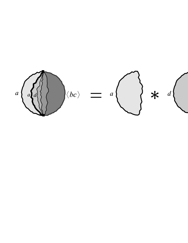
Figure 1: The disc graph contributing to $D_{a,\langle bc\rangle}$ can be decomposed into two discs along the contour line separating the domains of height $a$ and $d$ and connecting the two boundary operators. $D_{a,\langle bc\rangle}$ is therefore written as a $\ast$-product of $W_{a}$ and $D_{d,\langle bc\rangle}$.

This recursion relation allows us to express all the disc correlators $D_{a,\langle bc\rangle}$ in terms of the $2h-2$ basic correlators $D_{a,\langle a\,a\pm 1\rangle}$.

3.3.2 Bilinear functional equation for $D_{a,\langle ab\rangle}$

Let us next apply (75) to

$$G=e^{\ell^{\prime}X_{a}}\frac{1}{y-C_{ab}C_{ba}}C_{ab}\,.$$ (79)

Following the similar steps as before we obtain the loop equation

$$y\int_{0}^{\infty}d\ell\tilde{D}_{a,\langle ab\rangle}(\ell+\ell^{\prime},y)\tilde{D}_{b,\langle ba\rangle}(\ell,y)=y\tilde{D}_{a,\langle ab\rangle}(\ell^{\prime},y)-\tilde{W}_{a}(\ell^{\prime}).$$ (80)

After the Laplace transform with respect to $\ell$, it becomes

$$D_{a,\langle ab\rangle}(x,y)=\frac{1}{y}W_{a}(x)+D_{a,\langle ab\rangle}(x,y)\ast D_{b,\langle ba\rangle}(x,y).$$ (81)

This relation can also be understood from the viewpoint of the height configurations. Recall first of all that the $\langle ab\rangle$ boundary emanates contour lines separating the heights $a$ and $b$. Let us then think of a graph participating in $D_{a,\langle ab\rangle}$, and cut it along the contour line whose endpoint is the closest to the right end of the $\langle ab\rangle$ boundary. There may be no such contour line because the $\langle ab\rangle$ boundary may have zero length; in such a case the graph has constant boundary height $a$ and contributes to $W_{a}(x)$. Otherwise the graph can be decomposed into two pieces contributing respectively to $D_{a,\langle ab\rangle}$ and $D_{b,\langle ba\rangle}$. See Figure 2.

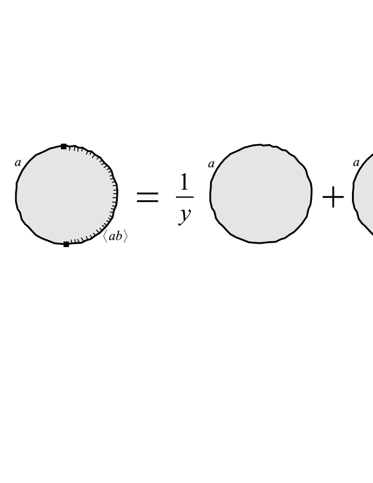
Figure 2: There are two types of graphs contributing to $D_{a,\langle ab\rangle}$. The graph may have $\langle ab\rangle$ boundary of length zero so that the whole boundary has height $a$. If $\langle ab\rangle$ boundary has nonzero length, one can cut it into two pieces contributing to $D_{a,\langle ab\rangle}$ and $D_{b,\langle ba\rangle}$, respectively.

These two possibilities correspond to the two terms in the RHS of (81).

The disc correlators $D_{a,\langle ab\rangle}$ and $D_{b,\langle ba\rangle}$ satisfy two relations, namely (81) and another equation obtained by exchanging $a$ and $b$. To get the more useful equation we take the discontinuity of these equations along the cut in the $x$-plane,

$$\begin{split}\text{Disc}D_{a,\langle ab\rangle}(x,y)=\frac{1}{y}\text{Disc}W_{a}(x)+D_{b,\langle ba\rangle}(-x,y)\text{Disc}D_{a,\langle ab\rangle}(x,y),\\ \text{Disc}D_{b,\langle ba\rangle}(x,y)=\frac{1}{y}\text{Disc}W_{b}(x)+D_{a,\langle ab\rangle}(-x,y)\text{Disc}D_{b,\langle ba\rangle}(x,y).\end{split}$$ (82)

Using these and taking into account the large-$x$ asymptotics of $W_{a}$ and $D_{a,\langle ab\rangle}$, we find

$$yD_{a,\langle ab\rangle}(x,y)D_{b,\langle ba\rangle}(-x,y)$$

$$-yD_{a,\langle ab\rangle}(x,y)-yD_{b,\langle ba\rangle}(-x,y)+W_{a}(x)+W_{b}(-x)~{}=~{}0.$$ (83)

By introducing

$$d_{a,\langle ab\rangle}(x,y)=\sqrt{y}\big{(}D_{a,\langle ab\rangle}(x,y)-1\big{)}$$ (84)

we can rewrite the equation (83) into a simpler form,

$$d_{a,\langle ab\rangle}(x,y)d_{b,\langle ba\rangle}(-x,y)+W_{a}(x)+W_{b}(-x)=y.$$ (85)

Here the normalization of $d_{a,\langle ab\rangle}$ is somewhat arbitrary, and we chose the symmetric normalization for simplicity.

3.4 Solution in the continuum limit

To study the continuum limit, we introduce a small parameter $\epsilon$ and the renormalized couplings $(\mu,\xi,\zeta)$ in the same way as we did for the $O(n)$ model,

$$\epsilon^{2}\mu=\kappa-\kappa^{*},\qquad\epsilon^{1/g}\xi=x-x^{*},\qquad\epsilon\zeta=y-y^{*}.$$ (86)

In [1, 7] the loop equations for $W_{a}(x)$ has been solved under the natural ansatz,

$$W_{a}(x)=S_{a}W(x).$$ (87)

$W(x)$ was then shown to satisfy the loop equation (13) for the resolvent of the $O(n)$ matrix model with $n=2\cos(\pi/h)$. So we borrow the solution from the $O(n)$ model under the identification

$$\theta=1-g=\frac{1}{h}.$$ (88)

We define the renormalized resolvent $w(\xi)$ in the same way as in (40). The solution in the continuum limit is given by

$$\xi=M\cosh\tau,\qquad w(\xi)=-\frac{M^{g}}{2g}\cosh g\tau.$$ (89)

Again, $M$ is related to $\mu$ via (42).

Now let us solve the loop equation (85) for the correlators $d_{a,\langle ab\rangle}$. First we need to determine the critical value of the $\langle ab\rangle$-boundary cosmological constant $y^{\ast}$. We require that $d_{a,\langle ab\rangle}$ and $d_{b,\langle ba\rangle}$ vanish at the critical point $(\kappa^{*},x^{*},y^{*})$ and find

$$y^{*}=W_{a}(0)+W_{b}(0)=(S_{a}+S_{b})W(0).$$ (90)

Next we renormalize the disc correlators near the critical point as

$$\begin{split}&d_{a,\langle ab\rangle}(x,y)=\epsilon^{\alpha_{a,\langle ab\rangle}/g}d_{a,\langle ab\rangle}(\xi,\zeta),\\ &\alpha_{a,\langle ab\rangle}+\alpha_{b,\langle ba\rangle}=g=1-\frac{1}{h}\,.\end{split}$$ (91)

The loop equation in the limit of small $\epsilon$ is

$$d_{a,\langle ab\rangle}(\xi,\zeta)d_{b,\langle ba\rangle}(-\xi,\zeta)+S_{a}w(\xi)+S_{b}w(-\xi)=\zeta.$$ (92)

By substituting (89) and

$$\zeta=\frac{M^{g}S_{1}}{2g}\cosh{g\sigma}$$ (93)

into (92), the loop equation finally becomes

$$\begin{split}&d_{a,\langle ab\rangle}\big{(}\tau-i\pi/2,\sigma\big{)}d_{b,\langle ba\rangle}\big{(}\tau+i\pi/2,\sigma\big{)}\\ &=\frac{M^{g}S_{1}}{g}\cosh\Big{(}\frac{g(\tau+\sigma)+\alpha_{ab}}{2}\Big{)}\cosh\Big{(}\frac{g(\tau-\sigma)+\alpha_{ab}}{2}\Big{)},\end{split}$$ (94)

where $\alpha_{ab}$ for $b=a\pm 1$ is given by

$$\alpha_{ab}=\pm\frac{i\pi}{2}\left(1-\frac{a+b}{h}\right)=-\alpha_{ba}.$$ (95)

The above equation has the same structure as (49), so the solution is given in terms of the Liouville boundary two-point functions. We can now use the formulae in Appendix A and B and determine the gravitational dimensions of the boundary changing operators

$$\Delta_{a,\langle ab\rangle} =\Delta_{a,a},\quad \Delta_{b,\langle ba\rangle} =\Delta_{1-b,-b}\quad \text{when }b=a+1,$$

$$\Delta_{a,\langle ab\rangle} =\Delta_{1-a,-a},\quad \Delta_{b,\langle ba\rangle} =\Delta_{b,b}\quad \text{when }b=a-1.$$ (96)

This implies that the boundary operators ${}^{a}\!B{}^{\langle a\,a+1\rangle}$ and ${}^{a}\!B{}^{\langle a\,a-1\rangle}$ in RSOS model have conformal weights $\delta_{a,a}$ and $\delta_{a-1,a}$, in full agreement with the result of Saleur and Bauer.

From the comparison of the loop equation (78) with (122), it follows that the correlators $d_{a,\langle bc\rangle}$ are all given by Liouville boundary two-point functions. The operators ${}^{a-L}\!B{}^{\langle a\,a+1\rangle}$ and ${}^{a+L}\!B{}^{\langle a\,a-1\rangle}$ are then shown to have conformal weights $\delta_{a,a+L}$ and $\delta_{a-1,a+L}$, respectively. By varying the integer parameters $a$ and $L$, the whole spectrum of boundary operators for this rational CFT is recovered. This result proves the conjecture of [13] on the scaling dimensions of boundary changing operators in the RSOS model.

4 The map between the two models

It has been known for a long time that the $O(n)$ model and SOS models are described by the same class of conformal field theories. In particular, the RSOS model with $h-1$ nodes was known to have the same partition function on the plane as the rational $O(n)$ model with $n=2\cos(\pi/h)$. Here we wish to explore this correspondence further, focusing mainly on the theories on the disc.

As was used in the previous section, the $O(n)$ model on the disc with Neumann boundary condition is equivalent to the RSOS model with fixed-height boundary condition. The disc partition functions are related via

$$W_{a}(x_{\text{RSOS}})=S_{a}W(x_{\text{O(n)}}).$$ (97)

In [8] it was shown that the $\langle ab\rangle$-type boundaries of RSOS model correspond to the JS boundaries of the $O(n)$ model labeled by integer $r$. The annulus partition functions of the $O(n)$ model with Neumann-JS boundary conditions were shown to agree with those of RSOS model with $a$-$\langle bc\rangle$ boundary conditions. It was also noticed there that one needs to introduce $L$ non-contractible loops on the annulus of the $O(n)$ model, corresponding to the distance between $a$ and $\langle bc\rangle$ labelling the two boundaries of the RSOS model.

Following their idea, we wish to relate the disc correlators of the two models on dynamical lattice. More explicitly, we will find out the relation between $D_{L}^{\parallel}$, $D_{L}^{\perp}$ of the $O(n)$ model and $D_{a+L,\langle a\,a-1\rangle}$, $D_{a-L,\langle a\,a+1\rangle}$ of the RSOS model. Our derivation of the relation is based on the loop equations and the diagrammatics of the matrix models, and does not rely on the continuum limit.

The first step is to relate the boundary cosmological constants. From the relation (97) we simply relate the $x$’s by

$$x_{\text{RSOS}}=x_{\text{O(n)}}$$ (98)

for Neumann boundary of the $O(n)$ model and the fixed height boundary in RSOS model. Similarly, it follows from (43) and (90) that the $y$’s for the $r$-th JS boundary and the $\langle ab\rangle$ boundary should be related via

$$\begin{split}y_{\text{O(n)}}&=\frac{y_{\text{RSOS}}}{S_{a}}\quad\big{(}\langle a,b\rangle=\langle r,r+1\rangle~{}~{}\text{or}~{}~{}\langle h-r,h-r-1\rangle\big{)},\\ y_{\text{O(n)}}&=\frac{y_{\text{RSOS}}}{S_{b}}\quad\big{(}\langle a,b\rangle=\langle r+1,r\rangle~{}~{}\text{or}~{}~{}\langle h-r-1,h-r\rangle\big{)}.\end{split}$$ (99)

4.1 Relations between Feynman graphs

Instead of finding the correspondence of disc correlators quickly from loop equations, let us explain how the correlators of the two matrix models should be related from the viewpoint of Feynman graph expansion.

The underlying idea is very simple. Each Feynman graph of the RSOS matrix model describes a dynamical lattice with a height assigned to every face, so that one can draw contour lines separating the domains of adjacent heights. If we focus only on the contour lines and forget about the heights, then what we get is nothing but the Feynman graph of the $O(n)$ matrix model. We thus compare each Feynman graph of the $O(n)$ matrix model with the sum over all the Feynman graphs of the RSOS model having the same contour line configuration but different height assignments.

4.1.1 Resolvents

To begin with, let us consider the relation between the resolvents of the RSOS and the $O(n)$ matrix models,

$$W_{a}(x)=S_{a}W(x).$$ (100)

Each graph contributing to $W_{a}(x)$ has the unique outermost domain of height $a$, and is inscribed by several subdomains of height $a\pm 1$. Each subdomain may be inscribed by several subdomains of adjacent heights, and by iterating this a finite number of times one can cover the entire disc. Now let us sum over all the height assignments in the interior. Using the rule explained after (65), we first assign $S_{a}$ to the outermost domain of height $a$. To each of its subdomains one can assign the height $a+1$ or $a-1$, which gives rise to a factor

$$\frac{S_{a+1}}{S_{a}}+\frac{S_{a-1}}{S_{a}}=2\cos\frac{\pi}{h}=n.$$ (101)

By repeating this and going step by step to the interior, one ends up with the Feynman graph of the $O(n)$ matrix model with a factor $n$ assigned to each loop. This explains the relation (100) at the level of the Feynman graph sum.

4.1.2 Disc correlators $D_{0}^{\perp}$ and $D_{a,\langle ab\rangle}$

Next, we use a similar argument to show the relation

$$D_{a,\langle ab\rangle}(x,y)=D_{0}^{\perp}\big{(}x,y/S_{a}\big{)},$$ (102)

where we assume $b=a+1$ for simplicity, and the JS boundary is expected to be labelled by $r=a$ from (99). To show this, we consider Feynman graphs contributing to the LHS with the power $1/y^{m+1}$. Such graphs have the $\langle ab\rangle$-boundary of length $m$, and there are therefore $m$ open contour lines ending on the $\langle ab\rangle$-boundary. If we cut the graph along these contours, it would decompose into $m_{a}$ pieces of boundary height $a$ and $m_{b}$ pieces of boundary height $b$, where $m_{a}+m_{b}=m+1$ and $m_{a}>0$. This means that the graphs have $m+1$ outermost domains of heights $a$ or $b$.

We now take the sum of such graphs over different height assignments in the interior but for a fixed contour line configuration, to obtain a graph of the $O(n)$ matrix model. Each contour line in the interior is assigned a factor $n$ in the same way as before. Collecting the factors associated to the outermost domains we find,

$$y^{-m-1}S_{a}^{m_{a}}S_{b}^{m_{b}}~{}=~{}\big{(}S_{a}/y\big{)}^{m+1}\times\big{(}S_{b}/S_{a}\big{)}^{m_{b}}.$$ (103)

We then deform the contour line configuration to a loop configuration by shrinking the $b$-part of the $\langle ab\rangle$-boundary as shown in Figure 3.

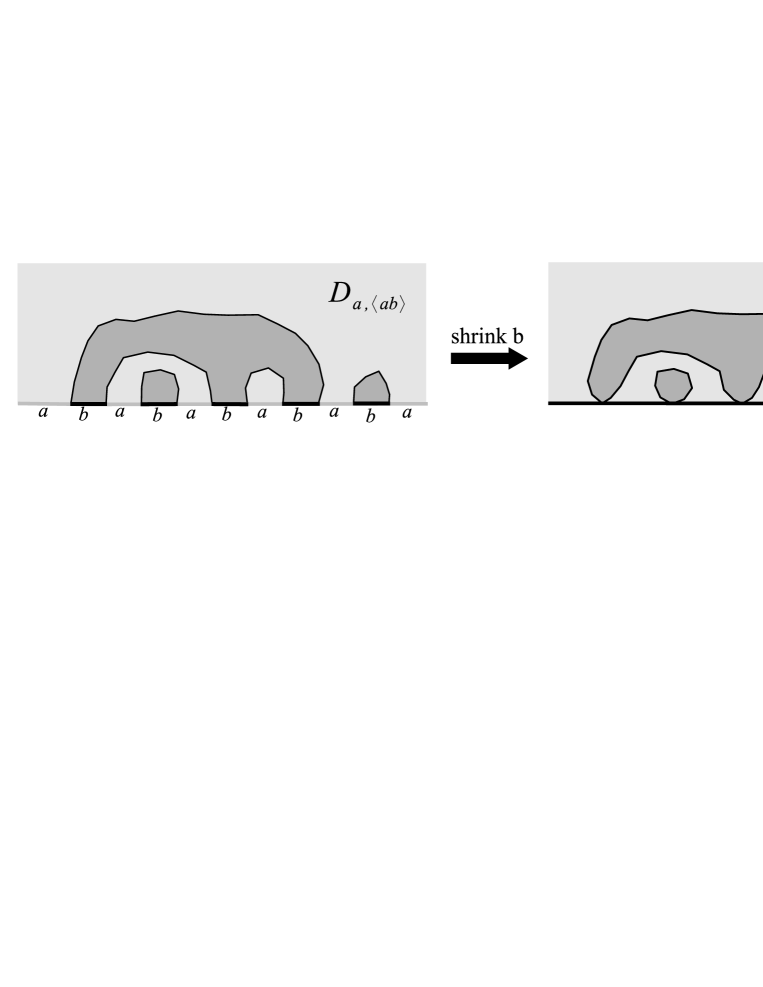
Figure 3: The graphs contributing to $D_{a,\langle ab\rangle}$ have open contour lines separating the domains of height $a$ and $b$. By shrinking the $b$ part of the $\langle ab\rangle$-boundary, those contour lines turn to form loops touching the boundary.

The $m$ open contour lines then turn into $m_{b}$ closed loops touching the boundary $m$ times in total. The expression for the weight (103) then implies that the $\langle ab\rangle$-boundary of the RSOS matrix model is mapped to the $k$-th JS boundary of the $O(n)$ model, with boundary cosmological constant $y/S_{a}$ and

$$k(a)=\frac{S_{a+1}}{S_{a}}=\frac{\sin{\pi(a+1)/h}}{\sin{\pi a/h}}.$$ (104)

Thus we have shown (102). It also implies $a=r$ in agreement with (99).

4.1.3 Disc correlators $D_{1}^{\parallel}$ and $D_{b,\langle ba\rangle}$

Using the same argument, let us next show the equation

$$D_{b,\langle ba\rangle}(x,y)=\frac{S_{b}}{y}\Big{(}W(x)+\frac{1}{k}D_{1}^{\parallel}\big{(}x,y/S_{a}\big{)}\Big{)}.$$ (105)

We again focus on the graphs contributing to the LHS with power $1/y^{m+1}$, which have $m$ open contour lines ending on the $\langle ba\rangle$-boundary. Such graphs have $m_{a}$ outermost domains of height $a$ and $m_{b}$ outermost domains of height $b$, with the condition

$$m_{a}+m_{b}=m+1,\qquad m_{b}>0.$$ (106)

We perform the sum over the height assignments in the interior and map the graphs to those of the $O(n)$ matrix model.

By shrinking the $b$-part of the $\langle ba\rangle$-boundary, we get the graph in the $O(n)$ matrix model which generically has one open line connecting the two boundary changing operators in addition to $m_{b}-1$ loops. They altogether touch the JS boundary $m-1$ times in total. It is important to notice that the open line can end on the JS boundary. We should therefore identify the boundary operators as the one-leg blobbed operators $\mathbb{Y}_{1}^{\parallel}$. The situation is illustrated in Figure 4.

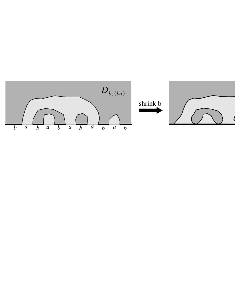
Figure 4: The graphs contributing to $D_{b,\langle ba\rangle}$ have open contour lines separating the domains of height $a$ and $b$. By shrinking the $b$ part of the $\langle ba\rangle$-boundary, those contour lines turn into some loops touching the boundary and a line connecting the two boundary-changing operators.

The graph of the $O(n)$ model we thus obtained has the following weight from the outermost domains,

$$y^{-m-1}S_{a}^{m_{a}}S_{b}^{m_{b}}~{}=~{}\big{(}S_{b}/y\big{)}\times\big{(}S_{a}/y\big{)}^{m}\times\big{(}S_{b}/S_{a}\big{)}^{m_{b}-1}.$$ (107)

The same graph and weight can be obtained from the Feynman graph expansion of the second term in the RHS of (105). Note that the additional factor $1/k$ is inserted because the line connecting the two $\mathbb{Y}_{1}^{\parallel}$ can be made from propagators of $Y_{1},\cdots$ or $Y_{k}$, leading to a factor $k$. The first term of the RHS, on the other hand, is the sum over the exceptional graphs of the RSOS model corresponding to $m=0$, namely, those graphs which have the $\langle ba\rangle$ boundary of length zero. The sum over such graphs is simply the leading term in the $1/y$-expansion of the LHS and therefore given by $W_{b}(x)/y$. This finishes the diagrammatic proof of (105).

The relations (102) and (105) can be used to show that the loop equations of the $O(n)$ matrix model (33) and the RSOS model (83) are mapped to each other. These relations also explain that the operators ${}^{a}\!B^{\langle a\,a+1\rangle}$ and ${}^{a+1}\!B^{\langle a+1\,a\rangle}$ have the same conformal weight as that of $\mathbb{S}_{0}^{\perp}$ and $\mathbb{S}_{1}^{\parallel}$ between the Neumann and the $k(a)$-th JS boundaries.

4.1.4 Disc correlators of $L$-leg operators

It is obvious how to extend the correspondence to the disc correlators of $L$-leg operators using the argument of summing over height configurations and shrinking the $b$-part of the $\langle ab\rangle$ boundary. We skip the details and present the final results.

$$\begin{split}D_{a-L,\langle a\,a+1\rangle}(x,y)&=S_{a-1}\cdots S_{a-L}\;\frac{(n-k-L)!}{(n-k)!}D_{L}^{\perp}(x,y/S_{a}),\\ D_{a+L,\langle a+1\,a\rangle}(x,y)&=\frac{S_{a+1}\cdots S_{a+L}}{y}\Big{(}W_{L}(x)+\frac{(k-L)!}{k!}D_{L}^{\parallel}(x,y/S_{a})\Big{)},\end{split}$$ (108)

where $W_{L}(x)$ is determined by the recursion relation

$$\text{Disc}W_{L+1}(x)=W_{L}(-x)\text{Disc}W(x),\qquad W_{1}(x)=W(x).$$ (109)

These include the results of the previous subsubsection as special cases. It is also easy to show that they relate the recursion relation of the $O(n)$ model (36) to that of the RSOS model (78). They also explain that the operator ${}^{a-L}\!B^{\langle a\,a+1\rangle}$ has the same conformal weight as $\mathbb{S}_{L}^{\perp}$ between the Neumann and the $k(a)$-th JS boundaries, and similarly for ${}^{a+L}\!B^{\langle a+1\,a\rangle}$ and $\mathbb{S}_{L}^{\parallel}$.

The first term in the second line of (108) is equal to the leading term in the $1/y$-expansion of the LHS, and the corresponding graphs have $\langle a+1\,a\rangle$ boundary of zero length. Therefore, $W_{L}(x)$ is a disc one-point function of a boundary operator with $L$ nested loops attached, corresponding to the fusion product of two $L$-leg operators. Such an operator should be described in terms of star operators [11]; the star operator $S_{L}$ is a source of $L$ open lines and is allowed to exist between two Neumann boundaries. In [11] its gravitational dimension was found to be $\Delta_{1,L+1}$, and the disc two-point functions were computed in the continuum limit. Our $W_{L}$ can be calculated in the same way. Using the standard parameterization $\xi=M\cosh\tau$ in the continuum limit we find,

$$W_{L}(\tau)=\prod_{k=1}^{L}\frac{\sin\pi g}{\sin\pi g(k+1)}\prod_{k=0}^{L}W\big{(}\tau+i\pi(L-2k)\big{)}.$$ (110)

5 Concluding remarks

In this paper we studied the new boundary condition of the $O(n)$ model proposed by Jacobsen and Saleur. By using the matrix model formulation, we were able to relate them to the boundary conditions of RSOS model with alternating heights. The loop equations turned out to be a very efficient tool in calculating the spectrum and the conformal weights of boundary changing operators.

Our techniques based on matrix model and loop equations are applicable to the analysis of more involved situations, such as discs with several JS boundaries labelled by different $k$. An interesting problem is to study the spectrum of boundary operators between two JS boundaries. (On a regular lattice this has been done in the recent work [25].)

Another natural and interesting question will be to ask how our results can be extended to the dilute phase. Since the lattice will no longer be packed densely by the loops, one would expect a conformal boundary condition for which some sites on the boundary have no open line attached. We will therefore need to generalize the JS boundary so that it can have vacancies. It will be an interesting problem to study the renormalization group flow for the fugacity associated to the vacancy. We hope to address this issue in the future.

Appendix A Gravitational dressing, Liouville theory and KPZ

Here we summarize some basic facts on conformal field theories coupled to gravity and boundary Liouville field theory. More details can be found in [11, 12] and the original paper [19, 26, 27].

Let us consider the ‘matter CFT’ of the central charge

$$c=1-\frac{6\theta^{2}}{1-\theta}<1.$$ (111)

When $\theta=1/h$ for a positive integer $h\geq 3$, the theory is rational and corresponds to the minimal model of the unitary series $(h-1,h)$. Turning on the gravity corresponds to summing over different metrics and topology of the two-dimensional space. After gauge fixing it amounts to coupling the CFT to the Liouville field $\phi$ and $bc$ ghost system.

Let us take the matter CFT to be the Coulomb gas model [14, 15] described by a scalar $\chi$. The vanishing of the total central charge puts a certain condition on the matter and the Liouville background charges $e_{0}$ and $Q$. We can parameterize them as

$$Q=\frac{1}{\mathfrak{b}}+\mathfrak{b}\,,\qquad e_{0}=\frac{1}{\mathfrak{b}}-\mathfrak{b}\,.$$ (112)

Here $\mathfrak{b}=\sqrt{1-\theta}$ is the Liouville coupling constant.

In this model we consider the matter field $e^{ie_{r,s}\chi}$ of conformal weight $\delta_{r,s}$. With a suitable gravitational dressing it becomes an operator of conformal weight one,

$$B_{r,s}=\frac{\Gamma(2\mathfrak{b}P_{r,s})}{\pi}\exp\left(ie_{r,s}\chi+\beta_{r,s}\phi\right).$$ (113)

Here various parameters are related as follows,

$$e_{r,s}=\frac{e_{0}}{2}-P_{r,s},\qquad\beta_{r,s}=\frac{Q}{2}-|P_{r,s}|,\qquad P_{r,s}=\frac{r}{2\mathfrak{b}}-\frac{s\mathfrak{b}}{2},$$ (114)

and $(r,s)$ is a pair of positive integers labelling degenerate representations of the matter CFT. The matter conformal weight $\delta_{r,s}$ is given by

$$\delta_{r,s}=\frac{(r/\mathfrak{b}-s\mathfrak{b})^{2}-(1/\mathfrak{b}-\mathfrak{b})^{2}}{4}\,.$$ (115)

Introducing gravitational dimension $\Delta\equiv(2P-e_{0})/2\mathfrak{b}$ and string susceptibility $\gamma_{\text{str}}\equiv-\theta/(1-\theta)$, one can write the KPZ scaling formula [28, 29, 30],

$$\delta=\frac{\Delta(\Delta-\gamma_{\text{str}})}{1-\gamma_{\text{str}}}.$$ (116)

Note that there is another way of gravitational dressing, $\tilde{\beta}=Q/2+|P|$, as was considered in [9]. As an example, the boundary identity operator can be dressed by $e^{\phi/\mathfrak{b}}$ instead of $e^{\mathfrak{b}\phi}$. This suggests that there are two boundary cosmological couplings, and one has a fractional dimension with respect to the other.

After turning on the gravity, correlators no longer depend on the positions of the operators inserted because one has to integrate over the positions of those operators. The dimensions of the operators therefore cannot be read from the position-dependence of their correlators. Instead, they should be read off from the dependence of correlators on the cosmological constant $\mu$. If we restrict to discs, then the amplitudes with $n$ boundary operators $B_{P_{i}}$ and $m$ bulk operators $V_{K_{j}}$ scale with $\mu$ as

$$\big{\langle}{}^{\xi_{1}}\!B_{P_{1}}\!\!{}^{\xi_{2}}\cdots{}^{\xi_{n}}\!B_{P_{n}}\!\!{}^{\xi_{1}}\;V_{K_{1}}\cdots V_{K_{m}}\big{\rangle}\propto\mu^{\gamma},$$ (117)

with

$$\gamma=\big{(}1-m-\frac{n}{2}\big{)}\big{(}1-\frac{\gamma_{\text{str}}}{2}\big{)}+\frac{1}{2\mathfrak{b}}\Big{(}\sum_{i=1}^{n}{|P_{i}|}+\sum_{j=1}^{m}{|K_{j}|}\Big{)}.$$ (118)

Of course, the gravitational dimensions of the operators can be read more explicitly from the more detailed form of the amplitudes.

As an example, let us consider a disc with two boundary segments, labelled by boundary cosmological constants $\zeta_{1}$ and $\zeta_{2}$ and connected by the operators ${}^{\zeta_{1}}\!B^{\zeta_{2}}$. In boundary Liouville theory, boundary cosmological constant $\zeta$ is the coefficient of the boundary interaction $e^{\mathfrak{b}\phi}$. Following [19] we use a parametrization of $\zeta$ similar to (48),

$$\zeta=\sqrt{\frac{\mu}{\sin{\pi\mathfrak{b}^{2}}}}\cosh{\mathfrak{b}^{2}\tau}.$$ (119)

The computation of the disc amplitude involves the disc two-point functions of the Liouville and matter CFTs. The Liouville and matter part of the correlator factorize, and the matter part gives only a $\zeta$-independent factor. The Liouville part is given by [19]

$$\big{\langle}{}^{\zeta_{1}}\!B_{P}{}^{\zeta_{2}}(x)\,{}^{\zeta_{2}}\!B_{P}{}^{\zeta_{1}}(0)\big{\rangle}_{\text{Liouville}}=A(P)d(|P|,\tau_{1},\tau_{2})|x|^{-2\beta(Q-\beta)}\,,$$ (120)

with

$$\begin{split}\ln d(P,\tau_{1},\tau_{2})=-\int_{-\infty}^{\infty}\frac{d\omega}{\omega}\left(\frac{\cos\omega\tau_{1}\cos\omega\tau_{2}\sinh 2\pi P\omega/\mathfrak{b}}{\sinh\pi\omega\sinh\pi\omega/\mathfrak{b}^{2}}-\frac{2P\mathfrak{b}}{\pi\omega}\right).\end{split}$$ (121)

Here $A(P)$ is a known function of $P$ and is related to the “leg factor” arising from different normalization of the wave functions. It is independent of $\tau$’s and therefore unimportant. On the other hand, the $\tau$-dependent part (121) is expressed in terms of the double-sine function of pseudo-periods $\mathfrak{b}$ and $1/\mathfrak{b}$ [31]. It satisfies an important shift relation involving both $P$ and $\tau_{i}$,

$$d(P,\tau_{1}+i\pi,\tau_{2})-d(P,\tau_{1}-i\pi,\tau_{2})\;\propto\;\sinh{\mathfrak{b}^{2}\tau_{1}}\,d(P-\mathfrak{b}/2,\tau_{1},\tau_{2}),$$ (122)

up to a $\tau$-independent factor. Shifting $P$ by $-\mathfrak{b}/2$ corresponds to changing the label of the operator from $(r,s)$ to $(r,s+1)$.

Appendix B Solving the loop equation

Here we solve the loop equation (49)

$$d_{1}\big{(}\tau\mp\frac{i\pi}{2},\sigma\big{)}d_{0}\big{(}\tau\pm\frac{i\pi}{2},\sigma\big{)}=CM^{g}\cosh\frac{g(\tau+\sigma)\pm\alpha}{2}\cosh\frac{g(\tau-\sigma)\pm\alpha}{2}\;.$$

We define the function $u_{a}(\tau,\sigma)$ by

$$d_{a}(\tau,\sigma)=\frac{\sqrt{C}}{2}M^{\alpha_{a}}\exp u_{a}(\tau,\sigma)$$ (123)

with $\alpha_{a}+\alpha_{b}=g$, and denote by $\hat{u}_{a}(\omega,\sigma)$ their Fourier transform with respect to $\tau$.

Let us take the log and the Fourier transform of the loop equation. Using

$$\int_{-\infty}^{\infty}d\tau e^{i\omega\tau}\log\Big{(}2\cosh\frac{g\tau+\alpha}{2}\Big{)}=-\frac{\pi e^{-i\alpha\omega/g}}{\omega\sinh(\pi\omega/g)},$$ (124)

the loop equation for $\hat{u}_{a}(\omega,\sigma)$ becomes algebraic,

$$e^{\pm\frac{\pi\omega}{2}}\hat{u}_{1}(\omega,\sigma)+e^{\mp\frac{\pi\omega}{2}}\hat{u}_{0}(\omega,\sigma)\;=\;-\frac{2\pi}{\omega}\frac{\cos\omega\sigma}{\sinh(\pi\omega/g)}e^{\pm i\omega\alpha/g}.$$ (125)

Solving this in favor of $\hat{u}_{a}$ and Fourier transforming back, we find

$$u_{a}(\tau,\sigma)~{}=~{}-\int_{-\infty}^{\infty}\frac{d\omega}{\omega}\frac{\cos\sigma\omega\cos\tau\omega}{\sinh\pi\omega\sinh\pi\omega/g}\sinh\Big{(}\frac{\pi\omega}{2}\pm\frac{i\alpha\omega}{g}\Big{)},$$ (126)

where plus sign is for $u_{1}$ and minus sign for $u_{0}$. One recognizes the same functional form as the Liouville boundary two-point function (121).

By comparing (126) with (121) one finds the value of $P$ for the boundary-changing operators. Then by using the scaling law (118) one can determine the exponents $\alpha_{0}$ and $\alpha_{1}$

$$2\mathfrak{b}P_{0}=\alpha_{0}=r\theta,\qquad 2\mathfrak{b}P_{1}=\alpha_{1}=1-\theta-r\theta.$$ (127)

Another way to find $\alpha_{a}$ is to analyze the two-point function at $\zeta=\mu=0$,

$$d(\xi,\zeta=0,\mu=0)\sim\xi^{\alpha_{a}}\sim e^{\alpha_{a}|\tau|}.$$ (128)

Setting $\sigma=i\pi/2g$ and $\tau\to\infty$ in (126), the dominant contribution to the integral is from the vicinity of the second order pole at $\omega=0$. Using

$$\int_{-\infty}^{\infty}\frac{d\omega e^{i\omega\tau}}{\omega^{2}}=-\pi|\tau|,$$ (129)

one finds $u_{a}\simeq 2\mathfrak{b}P|\tau|$ and recovers (127) again.

References

- [1] I. K. Kostov, “Strings with discrete target space,” Nucl. Phys. B 376, 539 (1992) [hep-th/9112059].
- [2] V. A. Kazakov, “Exact solution of the Ising model on a random two-dimensional lattice,” JETP Lett. 44, 133 (1986) [Pisma Zh. Eksp. Teor. Fiz. 44, 105 (1986)].
- [3] D. V. Boulatov and V. A. Kazakov, “The Ising model on random planar lattice: the structure of phase transition and the exact critical exponents,” Phys. Lett. 186B, 379 (1987).
- [4] B. Duplantier and I. Kostov, Conformal spectra of polymers on a random surface,” Phys. Rev. Lett. 61, 1433 (1988); Geometrical critical phenomena on a random surface of arbitrary genus,” Nucl. Phys. B 340, 491 (1990).
- [5] V. K. Kazakov, “Percolation on a fractal with the statistics of planar Feynman graphs: exact solution,” Mod. Phys. Lett. A 4, 1691 (1989).
- [6] I. K. Kostov, “ vector model on a planar random lattice: spectrum of anomalous dimensions,” Mod. Phys. Lett. A 4, 217 (1989).
- [7] I. K. Kostov, “The ADE face models on a fluctuating planar lattice,” Nucl. Phys. B 326, 583 (1989).
- [8] J. L. Jacobsen and H. Saleur, “Conformal boundary loop models,” Nucl. Phys. B 788, 137 (2008) [math-ph/0611078].
- [9] I. Kostov, “Boundary loop models and 2D quantum gravity,” J. Stat. Mech. 0708, P08023 (2007) [hep-th/0703221].
- [10] V. A. Kazakov and I. K. Kostov, “Loop gas model for open strings,” Nucl. Phys. B 386, 520 (1992) [hep-th/9205059].
- [11] I. K. Kostov, B. Ponsot and D. Serban, “Boundary Liouville theory and 2D quantum gravity,” Nucl. Phys. B 683, 309 (2004) [hep-th/0307189].
- [12] I. K. Kostov, “Boundary correlators in 2D quantum gravity: Liouville versus discrete approach,” Nucl. Phys. B 658, 397 (2003) [hep-th/0212194].
- [13] H. Saleur and M. Bauer, “On some relations between local height probabilities and conformal invariance,” Nucl. Phys. B 320, 591 (1989).
- [14] B. Nienhuis, “Exact critical point and critical exponents of models in two-dimensions,” Phys. Rev. Lett. 49, 1062 (1982).
- [15] B. Nienhuis, “Critical behavior of two-dimensional spin models and charge asymmetry in the Coulomb gas,” J. Statist. Phys. 34, 731 (1984) and in C. Domb and J. L. Lebowitz, “Phase transitions and critical phenomena. vol. 11,” London, Uk: Academic (1987) 210p.
- [16] A. Nichols, V. Rittenberg and J. de Gier, “One-boundary Temperley-Lieb algebras in the XXZ and loop models,” J. Stat. Mech. 0503, P003 (2005) [cond-mat/0411512]; A. Nichols, “The Temperley-Lieb algebra and its generalizations in the Potts and XXZ models,” J. Stat. Mech. 0601, P003 (2006) [hep-th/0509069]; A. Nichols, “Structure of the two-boundary XXZ model with non-diagonal boundary terms,” J. Stat. Mech. 0602, L004 (2006) [hep-th/0512273].
- [17] P. A. Pearce, J. Rasmussen and J. B. Zuber, “Logarithmic minimal models,” J. Stat. Mech. 0611, P017 (2006) [hep-th/0607232].
- [18] I. K. Kostov, “Thermal flow in the gravitational model,” hep-th/0602075.
- [19] V. Fateev, A. B. Zamolodchikov and A. B. Zamolodchikov, “Boundary Liouville field theory. I: Boundary state and boundary two-point function,” hep-th/0001012.
- [20] H. Saleur and B. Duplantier, “Exact determination of the percolation hull exponent in two dimensions,” Phys. Rev. Lett. 58, 2325 (1987).
- [21] G. E. Andrews, R. J. Baxter and P. J. Forrester, “Eight vertex SOS model and generalized Rogers-Ramanujan type identities,” J. Statist. Phys. 35, 193 (1984).
- [22] V. Pasquier, “Two-dimensional critical systems labelled by Dynkin diagrams,” Nucl. Phys. B 285, 162 (1987).
- [23] I. K. Kostov, “Solvable statistical models on a random lattice,” Nucl. Phys. Proc. Suppl. 45A, 13 (1996) [hep-th/9509124].
- [24] I. K. Kostov, “Gauge invariant matrix model for the A-D-E closed strings,” Phys. Lett. B 297, 74 (1992) [hep-th/9208053].
- [25] J. Dubail, J. L. Jacobsen and H. Saleur, “Conformal two-boundary loop model on the annulus,” arXiv:0812.2746.
- [26] B. Ponsot and J. Teschner, “Boundary Liouville field theory: Boundary three point function,” Nucl. Phys. B 622, 309 (2002) [hep-th/0110244].
- [27] K. Hosomichi, “Bulk-boundary propagator in Liouville theory on a disc,” JHEP 0111, 044 (2001) [hep-th/0108093].
- [28] V. G. Knizhnik, A. M. Polyakov and A. B. Zamolodchikov, “Fractal structure of 2d-quantum gravity,” Mod. Phys. Lett. A 3, 819 (1988).
- [29] F. David, “Conformal field theories coupled to 2D graviry in the conformal gauge,” Mod. Phys. Lett. A 3, 1651 (1988).
- [30] J. Distler and H. Kawai, “Conformal field theory and 2d quantum gravity or who’s afraid of Joseph Liouville?” Nucl. Phys. B 321, 509 (1989).
- [31] S. Kharchev, D. Lebedev and M. Semenov-Tian-Shansky, “Unitary representations of , the modular double, and the multiparticle q-deformed Toda chains,” Commun. Math. Phys. 225, 573 (2002) [hep-th/0102180].