An Experimental Analysis of Lemke-Howson Algorithm

Abstract

We present an experimental investigation of the performance of the Lemke-Howson algorithm, which is the most widely used algorithm for the computation of a Nash equilibrium for bimatrix games. Lemke-Howson algorithm is based upon a simple pivoting strategy, which corresponds to following a path whose endpoint is a Nash equilibrium. We analyze both the basic Lemke-Howson algorithm and a heuristic modification of it, which we designed to cope with the effects of a ‘bad’ initial choice of the pivot. Our experimental findings show that, on uniformly random games, the heuristics achieves a linear running time, while the basic Lemke-Howson algorithm runs in time roughly proportional to a polynomial of degree seven. To conduct the experiments, we have developed our own implementation of Lemke-Howson algorithm, which turns out to be significantly faster than state-of-the-art software. This allowed us to run the algorithm on a much larger set of data, and on instances of much larger size, compared with previous work.

1 Introduction

The computation of a Nash equilibrium for bimatrix games has attracted a lot of attention in recent years. The problem is of central importance in several theoretical and applied areas, and has many applications in different fields, like the social sciences, biology, economics, etc.

The computational complexity of this problem has been unknown for many years, to the point that in 2001 Papadimitriou [9] mentioned it as one of the most important open problems in computational complexity. Recently the problem has been proved complete for a complexity class, $PPAD$, which contains problems for which efficient algorithms are not believed to exist [2].

In spite of the interest on the problem, little work has been done to carry out an accurate evaluation of the performance of the algorithms actually used to solve it. In this paper we experimentally analyze Lemke-Howson algorithm, which is the best known algorithm for the computation of a Nash equilibrium for bimatrix games.

We provide a new implementation of this algorithm, which turns out to be significantly faster than state-of-the-art software, and give an account of its performance. This new implementation allowed us to experimentally analyze Lemke-Howson algorithm on a much larger set of sample data, and on instances of much larger size, compared with previous work.

We also develop a heuristic modification of Lemke-Howson algorithm, which reduces the computational inefficiency which may result from a ‘bad’ initial choice of the pivot. On uniformly random games, this heuristics significantly outperforms the basic Lemke-Howson algorithm. While Lemke-Howson takes a number of steps which is roughly proportional to a polynomial of degree 7 with respect to the game size (see Figure 2), the heuristics takes a linear number of steps (see Figure 2).

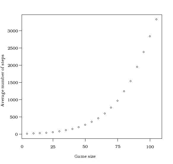
Figure 1: Average number of pivoting steps performed by LH as a function of the game size.

Figure 2: Average number of pivoting steps performed by our heuristics as a function of the game size.

This improvement makes it possible to compute equilibria in a reasonable time in games with size well beyond 1000 $\times$ 1000. The details can be found in the Appendix. Note that with standard Lemke-Howson algorithm, one can compute equilibria only on games of size up to a few hundreds (see Figure 3).

1.1 Other algorithms and previous experimental results

Lemke-Howson algorithm (LH from now on) is the most widely used algorithm for the computation of Nash equilibria in bimatrix games [4]. Nice descriptions of LH can be found in [16, 17].

More recently, new algorithms have been developed. Porter, Nudelman and Shoham [10] introduced a simple search method (PNS) based on the enumeration of all strategy supports. Sandholm, Gilpin and Conitzer introduced a different algorithm (MIP), based on Mixed Integer Programming [12].

A taxonomy of games can be found in [8]. The results obtained in [8, 10] show that two of the most challenging classes of games are the “uniformly random games” and the “covariant games”, which are the main objects of investigation in our paper.

Previous experimental works [10, 12] have shown that on games with small and balanced support, such as random games, PNS outperforms both MIP and LH, while on games with medium-size support LH outperforms both MIP and PNS. These experimental findings have been obtained by using the implementation of LH released in Gambit. A major difference with our work is that we have performed the experiments on a much larger set of sample data, and on instances of much larger size (see Section 3).

1.2 Organization of this paper

In Section 2 we give some background, and introduce the notation used in the paper. In Section 3 we briefly describe our implementation, giving account of its performance, and present our experimental results. In Section 4 we describe our heuristics, and give ample evidence of its efficiency on uniformly random games. In the Appendix we give a detailed description of our implementation of LH, and present some further experimental results on some classes of games, which, for lack of space, we had to omit from this extended abstract. The source code of our implementation can be found at http://allievi.sssup.it/game.

2 Background and Notation

We consider bimatrix games in normal form. These games are described in terms of two matrices, containing the payoffs of the two players. The rows (resp. columns) of both matrices are indexed by the row (resp. column) player’s pure strategies.

A mixed strategy consists of a set of pure strategies and a probability distribution (a collection of nonnegative weights adding up to one) which indicates how likely it is that each pure strategy is played. In other words, each player associates to her $i$-th pure strategy a number $p_{i}$ between $0$ and $1$, such that $\sum_{i}p_{i}=1$.

The pure strategies played with positive probability form the support of a mixed strategy.

Let us consider a two-player game, where the row (resp., column) player has $m$ (resp., $n$) pure strategies, and let $x$ be a mixed strategy of the row player, and $y$ a mixed strategy of the column player. Strategy $x$ is the $m$-tuple $x=(x_{1},x_{2},\dots,x_{m})$, where $x_{i}\geq 0$, and $\sum_{i=1}^{m}x_{i}=1$. Similarly, $y=(y_{1},y_{2},\dots,y_{n})$, where $y_{i}\geq 0$, and $\sum_{i=1}^{n}y_{i}=1$. Let now $A=(a_{ij})$ be the payoff matrix of the row player. The entry $a_{ij}$ is the payoff to the row player, when she plays her $i$-th pure strategy and the opponent plays the pure strategy $j$. According to the mixed strategies $x$ and $y$, the entry $a_{ij}$ contributes to the expected payoff of the row player with weight $x_{i}y_{j}$. The expected payoff of the row player can be evaluated by adding up all the entries of $A$ weighted by the corresponding entries of $x$ and $y$, i.e., the payoff is $\sum_{ij}x_{i}y_{j}a_{ij}$. This can be rewritten as $\sum_{i}x_{i}\sum_{j}a_{ij}y_{j}$, which can be expressed in matrix terms as$x^{T}Ay$. Similarly, the expected payoff of the column player is $x^{T}By$.

A pair $(x,y)$ is a Nash equilibrium if $x^{T}Ay\geq{x^{\prime}}^{T}Ay$, and $x^{T}By\geq x^{T}By^{\prime}$, for all stochastic vectors $x^{\prime}$ and $y^{\prime}$. If the pair $(x,y)$ is a Nash equilibrium, we say that $x$ (resp. $y$) is a Nash equilibrium strategy for the row (resp. column) player. It is well known that a Nash equilibrium in the mixed strategies always exists [7].

An equivalent definition is the following. A Nash equilibrium for a bimatrix game $(A,B)$ is a pair of mixed strategies $(x,y)$ such that each pure strategy is played with positive probability only if it is a best response to the other player’s mixed strategy (linear complementarity constraints):

$$\left\{\begin{array}[]{cc}\forall i\in\{1,\dots,m\}\text{ either }x_{i}=0\text{ or }(Ay)_{i}\geq max_{k}(Ay)_{k};\\ \forall j\in\{1,\dots,n\}\text{ either }y_{j}=0\text{ or }(x^{T}B)_{j}\geq max_{k}(x^{T}B)_{k}.\\ \end{array}\right.$$

To the set of equilibria, we add the artificial equilibrium $(0,0)$, where no strategy is played. It satisfies the linear complementarity constraint, but it is not a valid equilibrium.

We also say that a pair of mixed strategies form a quasi-equilibrium if all but one of the pure strategies played with positive probability satisfy the linear complementarity constraint.

Given a bimatrix game, and starting from any equilibrium (including the artificial equilibrium), LH follows a path in a graph whose vertices are the equilibria and the quasi-equilibria. Thus, starting from the artificial equilibrium, it is possible to reach a Nash equilibrium of any given game (see [17] for a detailed description of this process).

At each step, the state of the algorithm can be represented by the following system of inequalities, which define the space of the feasible mixed strategy profiles:

$$\left\{\begin{array}[]{cccc}\forall i\in\{1,\dots,m\}\text{ }x_{i}\geq 0;\\ \forall j\in\{1,\dots,n\}\text{ }y_{j}\geq 0;\\ \forall j\in\{1,\dots,n\}\text{ }(x^{T}B)_{j}\leq 1;\\ \forall i\in\{1,\dots,m\}\text{ }(Ay)_{i}\leq 1;\\ \end{array}\right.$$

Note that the formulation above has been obtained by applying a suitable scaling procedure where the maximum payoff is set to $1$, and the mixed strategies are scaled accordingly.

Following [17], these inequalities can be rewritten as:

$$\begin{pmatrix}a_{11}&\dots&a_{1n}\\ \vdots&\ddots&\vdots\\ a_{m1}&\dots&a_{mn}\\ -1&\dots&0\\ \vdots&\ddots&\vdots\\ 0&\dots&-1\\ \end{pmatrix}\begin{pmatrix}y_{1}\\ \vdots\\ y_{n}\\ \end{pmatrix}\leq\begin{pmatrix}1\\ \vdots\\ 1\\ 0\\ \vdots\\ 0\\ \end{pmatrix}$$

$$\begin{pmatrix}x_{1}&\dots&x_{m}\par\end{pmatrix}\begin{pmatrix}-1&\dots&0&b_{11}&\dots&b_{1n}\\ \vdots&\ddots&\vdots&\vdots&\ddots&\vdots\\ 0&\dots&-1&b_{m1}&\dots&b_{mn}\\ \end{pmatrix}\leq\begin{pmatrix}0&\dots&0&1&\dots&1\\ \end{pmatrix}$$

In order to describe the state of the algorithm at each step, we will use a structure called tableau, which consists of a representation of the inequalities above as equalities, obtained by introducing slack variables.

The transformation of inequalities into equalities of the tableau occurs as follows. Consider for example the inequality

$$a_{11}y_{1}+a_{12}y_{2}+\dots+a_{1n}y_{n}\leq 1$$

After introducing the slack variables, this inequality becomes:

$$a_{11}y_{1}+a_{12}y_{2}+\dots+a_{1n}y_{n}+r_{1}=1$$

Finally the equation is represented with all the non basic variables on the right hand side. Therefore, at the first step, we will have:

$$r_{1}=1-a_{11}y_{1}-a_{12}y_{2}-\dots-a_{1n}y_{n}.$$

In this equation, the variable on the left hand side is the basic variable, and the constant on the right hand side represents its current value. Starting from this representation, the algorithm proceeds via complementary pivoting steps, which allow the computation to move from a quasi-equilibrium to another one by changing each time one of the basic variables. This translates into a corresponding change in the tableau. The choice of the new basic variable is determined by the minimum ratio test - lines 12-15 of the pseudocode, which is in the Appendix. The complementary pivoting procedure terminates when all the strategies satisfy the complementary constraint, i.e., when an equilibrium is reached.

3 Experimental Results

3.1 Our implementation

The current state-of-the-art software for the computation of equilibria for games is Gambit [6]. It can be used to deal with extensive and normal form games. In particular, it is endowed with suitable command-line tools which allow the user to compute Nash equilibria for games given in normal form.

Being intended as a tool for high-level game theoretical analysis, Gambit does not provide accurate information on the efficiency of LH, e.g., on the number of complementary pivoting steps, and on properties of each execution. Therefore Gambit does not seem to be suitable for large scale experiments.

The need of low-level control on the computation and of a faster software tool lead us to develop our own implementation of LH. A detailed description of our implementation is given in the Appendix.

Figure 3 shows the average running time of LH, as a function of the game size. The games were generated using GAMUT, a suite of game generators [8].

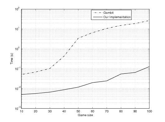
Figure 3: Average running time of LH. Our implementation (solid line) and Gambit (dotted line). On game sizes larger than 100$\times$100, a relevant fraction of games were not solved by Gambit within the capping time of 120 secs.

3.2 Uniformly Random Games

In this section we present the data collected for uniformly random games, i.e., games in which each payoff is chosen at random from the uniform distribution. We focus on the number of complementary pivoting steps, rather than on the execution time, the latter being too much implementation dependent.

When collecting the data, for each equilibrium computation, we kept track both of the equilibrium itself (the strategies played and the probability of playing each of them), and of the number of pivoting steps needed to reach it.

Figure 2 shows the average number of pivoting steps performed by LH: one can see that the number of steps grows polynomially (approximately according to a polynomial of degree 7) with the size of the game. The data has been obtained by running LH on 100,000 instances.

Figure 4: Support size distribution for games with 20 strategies per player (on the left), and 100 strategies per player (on the right). We take as support size the sum of the sizes of the supports of the strategies of both players.

Figure 4 shows the distribution of the support size of equilibria found by LH. We see that there is a small number of equilibria with large support size. Thus the behavior of LH agrees with the fact that the probability to find an equilibrium with a large support size is very low for (sufficiently large) uniformly random games. Although these findings only concern those equilibria which are found by LH, they show a close agreement with the theoretical results on the support of equilibria of random games [1].

To gather some further insights on the behavior of the algorithm, we analyzed the distribution of the number of pivoting steps performed by LH on games of three different sizes: 20, 40, and 100 strategies per player. For each size, we analyzed a large number of runs. More precisely, about 7.5 million runs for games with 20 and 40 strategies per player, and 700,000 runs for games with 100 strategies per player. Figure 5 shows the distribution of the number of steps for runs on 7.5 million games with 20 strategies per player.

Mode	Mean	1st Quartile	3rd Quartile	95% Quantile	99.5% Quantile
2	27.39	7	34	91	203

Figure 5: Number of steps performed by LH on uniformly random games of size 20

Figure 5 shows that the mode of the distribution of the number of complementary pivoting steps is $2$, which is the minimum number of steps needed to reach a pure equilibria. The data in Figure 5 illustrates that the distribution is very sparse: the third quartile is at 34 steps. Thus it is hard to make accurate predictions on the number of steps based on the game size. Indeed, in order to gather 99.5% of our statistical data, we had to go up to more than $200$ steps for games with 20 strategies per player. A closer look at the distribution gives us additional information on the behavior of the algorithm: two different distributions are interleaved, one for an even number of steps, and another one for an odd number of steps. Except for two, three, and four steps, the two interleaved distributions are almost geometrical.

Similar observations hold for larger games. Figure 6 shows the statistical data for games of size $40$ and $100$. Zooming on the distribution, we see that the two interleaved distributions still exist. As the games size increases these distributions do not change qualitatively. Indeed, while the mean and the sparseness of the distribution increase with the size, the shape stays the same.

Figure 6: Distribution of the number of steps performed by LH on games with 40 (left) and 100 (right) strategies per player. The y-axis is intentionally limited to ease the comparison of the two distributions.

3.3 Other classes of games

Further experimental results have been obtained on covariant games, as defined in [11]. This class contains families of instances which are harder to solve by LH than uniformly random games. For lack of space, the details are in the Appendix.

4 A heuristic improvement on Lemke-Howson algorithm

The number of steps taken by LH depends on the pivot it initially chooses. Since this choice is arbitrary, the algorithm might take a large number of steps, even on instances where there exist pivots on which it would terminate quickly. The performance of LH could be significantly improved if one knew in advance which pivot leads to the minimum number of steps.

In this section, we first analyze the performance of a clairvoyant algorithm (ND-Lemke-Howson) that chooses the best pivot and then executes LH starting from it. We then review a heuristics proposed by Porter, Nudelman and Shoham [10], which can be viewed as a simulation of ND-Lemke-Howson, and finally introduce a novel heuristics, which achieves a more efficient simulation of ND-Lemke-Howson.

4.1 ND-Lemke-Howson

We simulated ND-Lemke-Howson by executing the standard Lemke-Howson algorithm on all the possible pivots, and choosing the path with the minimum number of steps. The following is the pseudo-code description of this algorithm.

i = Best_pivot_to_start_from();

Lemke-Howson(pivot=i);

return equilibrium;

 

The first predictable result is that the distribution of the number of steps for ND-Lemke-Howson is much less sparse than the one for LH: for a large fraction of games it terminates in a very small number of steps. Figure 8 shows the distribution of the number of steps after 100,000 executions of ND-Lemke-Howson on 40$\times$40 random games. In particular, notice that the maximum number of steps is 12.

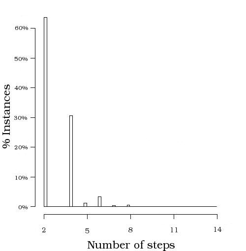
Figure 7: Number of steps performed by ND-Lemke-Howson algorithm for 40$\times$40 games.

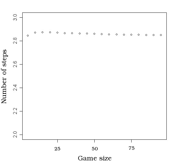
Figure 8: Mean of the number of steps performed by ND-Lemke-Howson as a function of the game size.

A significant difference between LH and ND-Lemke-Howson is that the average number of steps taken by ND-Lemke-Howson does not increase with the size of the game. The mean is almost stable at 2.8, and it slightly decreases as the game size increases (compare Figure 8 with Figure 2). This fact can be explained by observing that there is little correlation between the executions of LH for the same game on different pivots. And so, since the number of pivots increase linearly with size, the probability to find a short path increases accordingly.

4.2 Porter, Nudelman and Shoham heuristic approach

Porter, Nudelman and Shoham heuristics [10] simulates ND-Lemke-Howson by keeping track of all possible different executions of LH (two times the game size), and then performing a single pivoting step on each execution, until one of the paths reaches an equilibrium; the overhead with respect to ND-Lemke-Howson is approximately given by the number of steps performed by ND-Lemke-Howson multiplied by the number of possible pivots. The following is the pseudo-code implementation of this heuristics.

create 2 * dim different tableaux

while( true )
{
  for i = 1 to 2 * dim do
  {
    pivoting_step( tableaux[i] );
    if an equilibrium is found then
       return equilibrium;
    else
       continue;
  }
}

 

A significant implementation issue with this heuristics is that it requires a large amount of memory. Indeed, we have to store a different tableau for each pivoting path. Therefore the memory consumption is worse than LH by a factor of $2\cdot dim$. For a $dim\cdot dim$ game, one has to store $2\cdot dim$ tableaux, each of size quadratic in the game size, so that the overall memory consumption is cubic in the game size. This heuristics is thus unsuitable to compute equilibria for games with more than a few hundreds strategies per player.

4.3 A novel heuristics

We developed a slightly different heuristics, which avoids the problem of a large memory consumption, takes (on average) less pivoting steps, and is much easier to implement. This heuristics takes a parameter, which we call capping, that tells how many steps will be performed on each possible pivot before truncating the execution and starting it again on the following pivot, until some path reaches an equilibrium. If the length of the paths on every pivot is larger than the capping value, then we just execute LH on the last pivot. The following is the pseudo-code implementation of our heuristics.

for i = 1 to 2*dim - 1 do
{
  Lemke-Howson(pivot = i, max_steps = capping);

  if an equilibrium is found then
     return equilibrium;
  else
     continue;
}

if all paths have been truncated then
   Lemke-Howson(pivot = 2*dim, max_steps = INFTY);
   return equilibrium;

 

The memory consumption is clearly the same as in standard LH, since at each time step we use just one tableau. This allows our implementation to be executed even on games with thousands of strategies for each player. What makes this heuristics efficient is the fact that only a small fraction of games does not admit any short path.

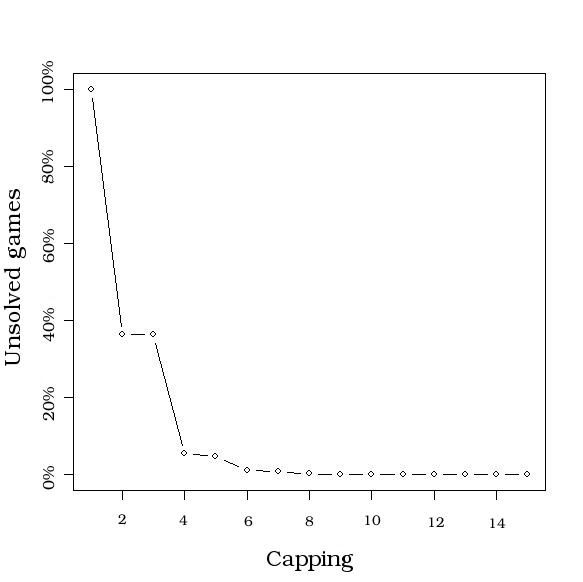
Figure 9: Fraction of 100$\times$100 games for which the heuristics is forced to execute LH on the last pivot, with respect to the capping parameter.

Figure 10: Average number of steps performed by our heuristics as a function of the capping parameter on 100$\times$100 games.

Figure 10 shows the fraction of games (of size 100$\times$100) for which the algorithm does not terminate before reaching the last pivot, as a function of the capping value. The lower is the capping value, the higher will be the probability to pivot on the last strategy. We can see that by choosing a capping value greater than 20 this probability is very small.

We performed an extended analysis to determine the best capping value for each game size on uniformly random games, and we have seen that the best value is approximately of 10 steps, and does not significantly change increasing the game size. Figure 10 shows how the average number of steps varies with the capping value for 100$\times$100 games. The performance improves significantly as the capping value approaches 10, and then gets slowly worse for larger values. The best performance (on average) is obtained by choosing a capping value of 10.

Figure 11 shows the distribution of the number of steps for our heuristics. It is similar to the distribution obtained for LH, although it is less sparse and not monotonic. Inside of it one can recognize many geometrical distributions, which represent the distribution of the feasible short paths that LH can generate from each pivot.

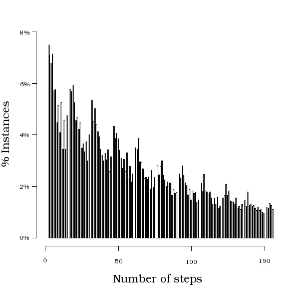
Figure 11: Number of steps performed by our heuristics, on 100$\times$100 games.

The data in Figure 2 shows the average number of steps of our algorithm. The average number of steps turns out to be linear, which is a drastic reduction compared with what we observed for LH (Figure 2).

Appendix A Our implementation

Our implementation of LH can either search for a Nash equilibrium in a normal form bimatrix game, executing LH on a given pivot strategy, or it can enumerate all equilibria reachable by LH starting from the artificial equilibrium.

We will only describe the first feature, the latter being of less importance to the experimental analysis we carry out in this paper.

A.1 The algorithm

A.1.1 Data Structures

The most relevant data structures are those used to store tableaux, equilibria, and lists of equilibria.

Since our main concern is execution time rather than memory consumption, we do not use a sparse matrix implementation of the tableau, but just a naive matrix representation. This allows us to efficiently access and update the tableau. To keep things simple, instead of using an array to keep track of the strategies which are in the basis, we store this information directly in the first column of the tableau. The second column represents the actual value of the variable in the basis for that row, while all the other entries represent the coefficients of all nonbasic variables.

For the sake of the reader, we now show an example of how a tableau looks like after being initialized. Consider the following game:

$$A=\left[\begin{array}[]{ c c }1&2\\ 3&4\\ 5&6\end{array}\right]\hskip 28.45274ptB=\left[\begin{array}[]{c c}7&8\\ 9&10\\ 11&12\end{array}\right]$$

The linear complementarity formulation is the following:

$$\left\{\begin{array}[]{llllll}s_{1}=1&{}&{}&{}&-x_{4}&-2x_{5}\\ s_{2}=1&{}&{}&{}&-3x_{4}&-4x_{5}\\ s_{3}=1&{}&{}&{}&-5x_{4}&-6x_{5}\\ s_{4}=1&-7x_{1}&-9x_{2}&-11x_{3}&{}&{}\\ s_{5}=1&-8x_{1}&-10x_{2}&-12x_{3}&{}&{}\end{array}\right.$$

where $s_{1},\ldots,s_{5}$ are the slack variables, and $x_{1},\ldots,x_{5}$ are the actual variables. This is the initial set up, where the equations represent the artificial equilibrium, with all the slack variables in the basis. The tableaux will be:

$$Tableau_{1}=\left[\begin{array}[]{ccccccc}-1&1&0&0&0&-1&-2\\ -2&1&0&0&0&-3&-4\\ -3&1&0&0&0&-5&-6\end{array}\right]$$

$$Tableau_{2}=\left[\begin{array}[]{ccccccc}-4&1&0&0&-7&-9&-11\\ -5&1&0&0&-8&-10&-12\end{array}\right]$$

We broke the tableau in two smaller independent tableaux, to simplify its update during the complementary pivoting steps. The first column represents the index of the basic variable for the given row. Positive indices are used for actual variables and negative ones for slack variables. The second column stores the value of that variable. All the other entries in the tableau are the coefficients of all the other variables, which are out of the basis. First come the coefficients of the slack variables, then those of the actual variables. For example, in the first tableau (representing the first three linear complementarity equations) columns 3 to 5 represent the coefficient of slack variables of indices 1 to 3 (these are all zeros, because all slacks are in the basis in the artificial equilibrium), while columns 6 and 7 are the coefficients of variables 4 and 5. All the other data structures of interest are used in the enumeration of all Nash equilibria reachable by LH. We use lexicographically sorted linked lists to store both equilibria and lists of equilibria, thus minimizing the time needed to check if an equilibrium had been already inserted in the list. Since we wish to keep the time to compare equilibria as low as possible, we used a null pointer implementation of the artificial equilibrium.

A.1.2 Pseudo-Code

In the following, we describe our implementation of LH.

[1]1 lemke_howson( bimatrix, tableaux, startpivot ) pivot = startpivot

while( true ) cur_tab = get_cur_tableau( pivot ) col_i = get_col_i( pivot )

for i = 1 to cur_tabeau.n_rows if( cur_tab[i][col_i] ¿ 0 ) continue;

ratio = -cur_tab[i][1] / cur_tab[i][col_i] if( ratio ¡ minimum_ratio ) minimum_ratio = ratio row_i = i

var_out = get_variable( cur_tab[row_i] ) col_i_out = get_col_i( var_out )

cur_tab[row_i][col_i] = 0 cur_tab[row_i][col_i_out] = -1 for i = 1 to cur_tab[row_i].length cur_tab[row_i][i] /= -cur_tab[row_i][col_i]

for i = 1 to cur_tab.n_rows if( cur_tab[i][col_i] != 0 ) for j = 1 to cur_tab[i].length cur_tab[i][j]+=cur_tab[i][col_i]*cur_tab[i][j]

cur_tab[i][col_i] = 0

pivot = -var_out if(pivot == startpivot or pivot == -startpivot) break

equilibrium = get_equilibrium( tableaux ) return equilibrium

The algorithm acts on the two matrices describing the game, the strategy to pivot on at the first step, and the two tableaux. In the first execution the two tableaux will be built from the artificial equilibrium, while in any subsequent execution, the algorithm can start from an arbitrarily chosen equilibrium.

The body of the algorithm consists of an infinite loop (lines 4 to 39 above) where the complementary pivoting steps are performed: the algorithm exits from the cycle when the variable which is going to leave the basis is either the starting pivot or its corresponding slack variable (line 37). Indeed, this means we are at an actual Nash equilibrium. At the end of the pivoting steps, we only have to extract the equilibrium from the tableau: this is done by looking at which strategies are in the basis, and what is the value of the corresponding variable in the tableau. We can then recover the actual Nash equilibrium, after normalizing these values so that the sum of the strategies played by each player is 1. This task is performed by the get_equilibrium function, called after the pivoting steps at line 41.

We now analyze the implementation of the complementary pivoting steps. We first select the tableau which contains our pivot, and then determine the column which corresponds to our pivoting strategy (lines 5 and 6).

The complementary pivoting step consists of two phases: (1) determining the variable going out of the basis (and the row in the tableau associated with it), and (2) updating the tableau according to the new basis. In phase (2), the update involves both the row in the tableau determined in the phase (1), and the rest of the coefficients, on the grounds of the expression of our new basic variable as a linear combination of nonbasic variables.

The minimum ratio test (lines 8 to 17) is done by evaluating the ratio between the value of all the variables in the basis and the coefficient of the variable entering the basis (our pivot). This ratio is obviously calculated only in those rows where the coefficient of the pivot is negative (lines 9-10). The row which minimizes this ratio is chosen, along with the variable leaving the basis (lines 13-16).

The update of the tableau is done as follows. First of all we determine the index of the column of the variable leaving the basis (lines 19-20). Then, we update the row involved in the change of the basic variable: to do this we set the coefficient of the pivot variable to zero (because now it is a basic variable), the coefficient of the variable going out of basis to -1 (we are, in fact, moving that variable from the left hand side of the equation represented by this row to the right hand side). After dividing all the other coefficients by the coefficient of the pivot, we get the final values (lines 22 to 25). Finally, we update all the other rows in the tableau (lines 27 to 34).

The complementary pivoting rule forces the choice of the next pivoting variable: it will be the complement of the variable which just exited the basis (line 36). Therefore the algorithm follows a path of quasi-equilibria with a duplicate label, i.e., a label for which both the variable and its slack are in basis, and a missing label. The process stops when the variable going out of the basis will be either our initial pivot or its slack (line 37-38).

A.2 Performance

A.2.1 The computational environment

We executed our program on a SUN X4200 workstation, with 2 AMD Opteron 2.6 Ghz dual core processors, 4GB of DDR PC3200 RAM, 1MB L2 Cache per core. This workstation runs Debian GNU-Linux Etch amd64 on a Xen 3.0.2 virtual machine. The program was compiled with gcc 4.0.3 with ’-O2 -mtune=x86-64’ as compilation options.

A.2.2 Some Issues with Gambit implementation

For the sake of comparing our implementation of LH with the one provided within Gambit, we had to make some minor modifications to Gambit code. In our experiments, we sometimes execute a single LH run pivoting on a given variable. On the other hand, Gambit’s tool gambit-lcp only allows the user to enumerate all equilibria reachable by LH starting from the artificial equilibrium. Therefore, we modified Gambit code, and added the option above. Moreover, we made other minor changes in order to gather more detailed information on the execution of the algorithm, i.e. variables entering and leaving the basis and number of pivoting steps performed by the algorithm itself.

A.2.3 Performance of our heuristics

Figure 12 shows the performance of our heuristics, on uniformly random games.

Game Size	Running Time
200	0.1699s
300	0.6664s
400	1.6184s
500	3.1029s
600	5.1076s
700	8.7794s
800	10.4485s
900	16.7848s
1000	27.7215s
1100	32.3306s
1200	57.6926s

Figure 12: Average running time of our heuristics with respect to the game size.

One can see that, on a standard PC, one can compute equilibria of games with size up to 1200$\times$1200 under 1 min.

Appendix B Other classes of games

B.1 Covariance Games

Following [8], we analyzed the performance of LH on the random game model of Rinott and Scarsini ([11]), in which the payoffs are drawn from two multivariate normal random distribution with a covariance parameter $\rho$ varying in the range [-1, 1]. A covariance of 1 means that the two players share the same payoffs, while a covariance of -1 means that the game is zero-sum and the payoffs have a minimal correlation. For a game of size 20, the behavior of LH changes as shown in Figure 13.

Figure 13: Average number of steps performed by LH on a 20$\times$20 covariant game with respect to the covariance.

When $\rho>0$, the number of steps of LH decrease as $\rho$ increases. This might be explained by the theoretical analysis in [11], which shows that for a positive value of $\rho$, the probability of finding a pure strategy equilibrium increases as a monotonic function of $\rho$. When $\rho<0$, the mean, mode and median of the distribution of the number of steps increase dramatically as $\rho$ decreases, reaching a maximum for $\rho=-0.7$. Similar results hold for games of different size.

It is interesting to look at the distribution of the support size of the equilibria reached by LH on 20$\times$20 and 100$\times$100 games for $\rho=-0.7$ (Figure 14). The graph resembles a normal distribution centered at a value which is slightly less than half the size of the game.

Figure 14: Support size distribution for covariant games with 20 strategies per player (on the left), and 100 strategies per player (on the right) for $\rho=-0.7$.

Comparing Figure 14 with Figure 4, we see that the equilibria found by LH on covariant games tend to have a greater average support size. The resulting distribution of the number of steps turns out to be shifted to the right with respect to what happens for uniformly random games (see Figure 15).

Figure 15: Distribution of the number of the steps for covariant games with 20 strategies per player (on the left), and 100 strategies per player (on the right) for $\rho=-0.7$.

Therefore, it is unlikely that any heuristics of the kind discussed in this paper could possibly do better than LH.

References

- [1] I. Barany, S. Vempala, A. Vetta, Nash Equilibria in Random Games. FOCS 2005, pp. 123-131.
- [2] X. Chen, X. Deng, Settling the Complexity of 2-Player Nash-Equilibrium. Electronic Colloquium on Computational Complexity (ECCC) 140 (2005).
- [3] S. Govindan and R. Wilson. A Global Newton method to compute Nash equilibria. J. of Economic Theory, 110:65–86 (2003).
- [4] C. E. Lemke, J. T. Howson. Equilibrium Points in Bimatrix Games. Journal of the Society for Industrial and Applied Mathematics, 12, pp. 413-423 (1964).
- [5] O. L. Mangasarian and H. Stone. Two-person nonzero-sum games and quadratic programming. Journal of Mathematical Analysis and Applications, 9:348-355 (1964).
- [6] R. D. McKelvey, A. M. McLennan, and T. L. Turocy. Gambit: Software Tools for Game Theory, Version 0.2007.01.30 http://econweb.tamu.edu/gambit (2007).
- [7] J. F. Nash. Non-cooperative Games. Annals of Mathematics, 51, pp. 286-295 (1951).
- [8] E. Nudelman, J. Wortman, K. Leyton-Brown, Y. Shoham. Run the GAMUT: A Comprehensive Approach to Evaluating Game-Theoretic Algorithms. AAMAS-2004: 880-887.
- [9] C. H. Papadimitriou. Algorithms, games, and the internet. STOC 2001: 749-753.
- [10] R.Porter, E. Nudelman, Y. Shoham. Simple Search Methods for Finding a Nash Equilibrium. Proceedings of the National Conference on Artificial Intelligence, 2004, 664-669
- [11] Y. Rinott, M. Scarsini. On the number of pure strategy Nash equilibria in random games. Games and Economic Behavior, 33, 2000.
- [12] T. Sandholm, A. Gilpin, V. Conitzer. Mixed-Integer Programming Methods for Finding Nash Equilibria. Proceedings of the National Conference on Artificial Intelligence, 2005, 495-501
- [13] R. Savani. Challenge Instances for NASH. CDAM Research Report LSE-CDAM-2004-14 (2004).
- [14] R. Savani, B. von Stengel. Exponentially Many Steps for Finding a Nash Equilibrium in a Bimatrix Game. Proceedings of 45th Annual Symposium on Foundations of Computer Science, 2004, pp. 258-267.
- [15] R. Savani and B. von Stengel. Hard-to-Solve Bimatrix Games. Econometrica 74, 397-429 (2006).
- [16] L. S. Shapley. A note on the Lemke-Howson Algorithm. Mathematical Programming Study 1: Pivoting and Extensions, 1974, pp. 175-189.
- [17] B. von Stengel. Computing Equilibria for Two-person Games. Handbook of Game Theory, vol.3, eds. R. J. Aumann e S. Hart, North-Holland, Amsterdam, 2002, cap. 45, pp. 1723-1759.