Phenomenology of SUSY with scalar sequestering

Abstract:

The defining feature of scalar sequestering is that the MSSM squark and slepton masses as well as all entries of the scalar Higgs mass matrix vanish at some high scale. This ultraviolet boundary condition - scalar masses vanish while gaugino and Higgsino masses are unsuppressed - is independent of the supersymmetry breaking mediation mechanism. It is the result of renormalization group scaling from approximately conformal strong dynamics in the hidden sector. We review the mechanism of scalar sequestering and prove that the same dynamics which suppresses scalar soft masses and the $B_{\mu}$ term also drives the Higgs soft masses to $-|\mu|^{2}$. Thus the supersymmetric contribution to the Higgs mass matrix from the $\mu$ term is exactly canceled by the soft masses. Scalar sequestering has two tell-tale predictions for the superpartner spectrum in addition to the usual gaugino mediation predictions: Higgsinos are much heavier ($\mu\gtrsim$ TeV) than scalar Higgses ($m_{A}\sim$ few hundred GeV), and third generation scalar masses are enhanced because of new positive contributions from Higgs loops.

1 Introduction

Tree level sum rules for superpartner masses and the supersymmetric flavor problem motivate the study of models in which supersymmetry breaking occurs in a hidden sector and is communicated to the visible sector through mostly flavor universal interactions. Below the mass scale of the communication mechanism, the visible and hidden sectors are only coupled through higher dimensional operators. To compute the spectrum of superpartner masses in the visible sector one must renormalize these operators from the communication scale, $M_{*}$, down to the superpartner mass scale.

It is by now well-appreciated that hidden sector interactions can have very large effects on this renormalization. For example, in models with conformal sequestering [1, 2] [3] [4, 5, 6] all MSSM superpartner masses are strongly suppressed relative to the gravitino mass so that anomaly mediation becomes dominant. In more general models hidden sector renormalization is not universal, and several new hidden-sector dependent parameters are needed to parametrize the superpartner spectrum [7] (for recent work in this direction see [8, 9]). When the hidden sector is strongly coupled and approximately conformal between $M_{*}$ and a lower scale $M_{\text{int}}$ then some supersymmetry breaking operators may be so strongly suppressed that they do not contribute to superpartner masses. In such cases the number of effective parameters may actually be reduced.

For example, references [10, 11] showed that if certain inequalities between anomalous dimensions in the hidden sector are satisfied then the running scalar masses evolve to be negligibly small compared to gaugino masses at $M_{\text{int}}$, and the ultraviolet values of the scalar masses become irrelevant parameters. We refer to this suppression of scalar masses as scalar sequestering. The squark and slepton mass spectrum of scalar sequestering resembles that of gaugino mediation [12, 13] [14, 15], however as was pointed out in [10, 11] there are important differences for the Higgs sector. The running Higgs scalar mass matrix in the MSSM is

$$\begin{pmatrix}m_{H_{u}}^{2}+|\mu|^{2}&B_{\mu}^{*}\\ B_{\mu}&m_{H_{d}}^{2}+|\mu|^{2}\end{pmatrix}\;,$$ (1)

where $\mu$ is the usual supersymmetry preserving $\mu$-parameter while $m_{H_{d}}^{2}$, $m_{H_{u}}^{2}$ and $B_{\mu}$ are supersymmetry breaking. In the simplest attempts at solving the $\mu$ problem by coupling the Higgs doublets directly to messenger fields one often finds that $m_{H_{u}}^{2},m_{H_{d}}^{2},B_{\mu}\gg|\mu|^{2}$. This is problematic [16] because the experimental lower bound on Higgsino masses requires $|\mu|>m_{Z}$ whereas naturalness of the Higgs potential gives $m_{Z}^{2}\gtrsim\text{Min}\left[m_{H_{u}}^{2},m_{H_{d}}^{2},B_{\mu}\right]$. This problem can be solved by scalar sequestering. We will give a general proof that the same dynamics which sequesters the squark and slepton masses also sequesters the Higgs scalar mass matrix while leaving the $\mu$ term unaffected.

To summarize, scalar sequestering predicts a distinct pattern of soft parameters at the scale $M_{\text{int}}$. The non-vanishing parameters are

$$\mu,\quad a_{t},a_{b},a_{\tau},\quad M_{1},M_{2},M_{3},\quad m_{H_{u}}^{2}=m_{H_{d}}^{2}=-|\mu|^{2}\;,$$ (2)

where $M_{i}$ are the gaugino masses and $a_{i}$ are the A-terms. Below $M_{\text{int}}$ the interactions of the hidden sector turn off (by definition of $M_{\text{int}}$), and the running is determined by the MSSM interactions alone.

The boundary values for the soft masses in Eq. (2) have several interesting consequences. Firstly, the fact that the soft scalar masses squared vanish at $M_{\text{int}}$ ameliorates the supersymmetric flavor problem. Flavor violation which may have been imprinted on the scalar mass operators at higher energies (for example by a messenger sector which is not flavor-universal) is rendered harmless by the sequestering. On the other hand, A-terms are not sequestered by hidden sector interactions, and large flavor violation in the A-terms must be avoided. The boundary values in Eq. (2) also significantly improve supersymmetric CP problem. The fact that $B_{\mu}$ vanishes at $M_{\text{int}}$ and our assumption of universal gaugino masses allow one to rotate away most of the flavor-universal CP violating phases. Only the phases of A-terms remain and the supersymmetric CP problem is greatly reduced [17].

Secondly, the fact that the entire scalar Higgs mass matrix vanishes at $M_{\text{int}}$ while $\mu$ remains large leads to two unique predictions for the superpartner spectrum at the TeV scale: in this model consistent electroweak symmetry breaking requires $\mu\gtrsim 1$ TeV and therefore heavy Higgsinos. But at tree level the Higgs scalar masses do not grow with $\mu$ and numerically we find $m_{A}^{2}\ll|\mu|^{2}$ throughout parameter space. In addition, the negative Higgs soft masses give positive contributions to the running of the third generation scalar masses. For example, we expect that the sum of the masses of the two stau mass eigenstates is larger than the sum of the selectron or smuon masses.

Finally, the fact that there are fewer non-vanishing parameters at $M_{\text{int}}$ increases the models’ predictivity. For example, if one also assumes unified gaugino masses and A-terms then the superpartner spectrum depends on only three free parameters.

The focus of our paper is to determine the superpartner mass spectrum and phenomenology which follow from the boundary condition in Eq. (2). Section 2 and the Appendix contain a review of hidden sector running and the derivation of the predictions $m_{H_{u}}^{2}=m_{H_{d}}^{2}=-|\mu|^{2}\;,\ B_{\mu}=0$, and $m_{Q}^{2}=m_{U}^{2}=m_{D}^{2}=m_{L}^{2}=m_{E}^{2}=0$. In Section 3 we find the viable region of parameter space and derive the spectrum for a sample point which satisfies all phenomenological constraints. In Section 4 we conclude and discuss future directions.

2 A peculiar spectrum at the intermediate scale

In this Section we review the theoretical framework which leads to the predicted relations for soft masses shown in Eq. (2). The basic idea is that this pattern of soft masses is a result of strong renormalization from hidden sector interactions. This makes it largely independent of the mediation mechanism operating at high scales.

We begin by assuming that there is some mediation mechanism between the visible and hidden sectors which generates a set of higher dimensional operators coupling the two sectors. The higher dimensional operators are suppressed by a scale which we denote by $M_{*}$. For example, in minimal supergravity, this scale is the Planck scale. In gauge mediation it is the messenger scale times $16\pi^{2}$. At weak coupling, and suppressing indices labeling different hidden sector operators, the most relevant hidden-visible couplings are of the form

$$\int\!\!\!d^{4}\theta\ \frac{\mathcal{R}}{M_{*}^{2}}Q^{\dagger}Q+\frac{\mathcal{X^{\dagger}}}{M_{*}}H_{u}H_{d}+\frac{\mathcal{R}}{M_{*}^{2}}H_{u}H_{d}+\ \text{h.c.}$$ (3)

$$+\int\!\!\!d^{2}\theta\ \frac{\mathcal{X}}{M_{*}}WW+\frac{\mathcal{X}}{M_{*}}QU^{c}H_{u}+\text{h.c.}\ .$$ (4)

Here $Q$ stands for any of the MSSM matter chiral superfields, $W$ stands for the MSSM gauge field strength superfields, $\mathcal{X}$ stands for hidden sector chiral operators, and $\mathcal{R}$ for real superfield operators of the hidden sector. The hidden sector operators may be elementary superfields or composite. $\mathcal{R}$ may contain products of a chiral and an anti-chiral operators $\mathcal{X^{\dagger}\!X}$, but in general $\mathcal{R}$ is a sum of operators, some of which can be written as such products and some which cannot. The powers of $M_{*}$ in the denominators have been chosen according to engineering dimensions so that the operator coefficients would have no further mass dimensions if $\mathcal{X}$ were a free chiral superfield $X$ and $\mathcal{R}$ were the product $X^{\dagger}X$. The real scaling dimensions of these operators are quite different from the engineering dimensions and are discussed below.

Ignoring any renormalization effects for the moment, we obtain the soft masses of the MSSM by replacing the hidden sector operators by vacuum expectation values (VEVs) for their auxiliary components

$$\langle\frac{\left.\mathcal{X}\right|_{F}}{M_{*}}\rangle=\frac{F}{M_{*}}\quad\quad\quad\langle\frac{\left.\mathcal{R}\right|_{D}}{M_{*}^{2}}\rangle=\frac{D}{M_{*}^{2}}\ .$$ (5)

The couplings in Eq. (3) become scalar masses, a $\mu$-term and $B_{\mu}$ whereas the couplings in Eq. (4) become gaugino masses and A-terms, respectively. Without any strong renormalization effects from the hidden sector a phenomenologically successful model requires $D\sim F^{2}$.

Note that we have omitted any terms of the form $\mathcal{X}Q^{\dagger}Q$ from Eq. (3) because they can be removed by a field redefinition. We discuss this field redefinition in more detail in the Appendix.

We now turn to the renormalization of the couplings in Eqs. (3) and (4) due to hidden sector interactions. We work in the holomorphic basis for hidden sector fields so that supersymmetric non-renormalization theorems are manifest.

An operator which is chiral or anti-chiral in hidden sector fields (i.e. an operator which depends on $\mathcal{X}$ or $\mathcal{X}^{\dagger}$ only) is not renormalized by purely hidden sector interactions in the holomorphic basis for hidden sector fields (see [10] for a proof). This immediately implies that the operators for gaugino masses and A-terms in Eq. (4) and the $\mu$ term in Eq. (3) are not renormalized by hidden sector interactions. This non-renormalization theorem extends to the actual gaugino masses, $A$-terms and and the $\mu$-term if they are expressed in terms of the expectation value for the holomorphic operator $\mathcal{X}$.

The operators which involve $\mathcal{R}$ are not protected from renormalization. They receive anomalous dimensions from hidden sector interactions which can have either sign [10] and are not calculable at strong coupling. The crucial dynamical assumption that underlies our framework is that these anomalous dimensions are large and positive [10, 11, 18]. Then all operators involving $\mathcal{R}$ are strongly suppressed at low energies. More precisely, we assume that the hidden sector is governed by a strongly coupled approximate fixed point below the scale $M_{*}$ and down to the scale $M_{\text{int}}$. Any operator in the low energy effective Lagrangian involving $\mathcal{R}$ will then be suppressed by a factor of $(M_{\text{int}}/M_{*})^{{\gamma_{\mathcal{R}}}}$ where ${\gamma_{\mathcal{R}}}$ is the anomalous dimension of the operator $\mathcal{R}$. When ${\gamma_{\mathcal{R}}}$ is of order one and the range of scales over which the strong hidden sector interactions operate is large, then all operators involving $\mathcal{R}$ have small coefficients at $M_{\text{int}}$, and their contributions to the running superpartner masses at $M_{\text{int}}$ can be neglected. This is nice for two reasons:

• The operators of the form $\frac{\mathcal{R}}{M_{*}^{2}}Q^{\dagger}Q$ may have non-trivial flavor structure from flavor physics in the ultraviolet. The resulting mass matrices for squarks and sleptons violate flavor and lead to flavor changing neutral currents which are tightly constrained by experiment. Hidden sector running suppresses such flavor violation and might therefore make some flavor-violating mediation mechanisms viable.

• Electroweak symmetry breaking requires that the coefficient of the operator $\frac{\mathcal{R}}{M_{*}^{2}}H_{u}H_{d}$ which gives rise to the $B_{\mu}$ term after supersymmetry breaking is small. More specifically, one needs $B_{\mu}\sim M_{\text{susy}}^{2}/\tan\beta$ in the infrared. A small coefficient for $\frac{\mathcal{R}}{M_{*}^{2}}H_{u}H_{d}$ is exactly what our renormalization factor predicts. Note however that our mechanism predicts small $B_{\mu}$ at $M_{\text{int}}$, whereas electroweak symmetry breaking requires small $B_{\mu}$ at the TeV scale. Therefore MSSM running below $M_{\text{int}}$ should not generate very large contributions to $B_{\mu}$. This will play a significant role in Sec. 3.

Given our assumptions about the anomalous dimensions of $\frac{\mathcal{R}}{M_{*}^{2}}$ a very simple and attractive picture emerges: at the scale $M_{\text{int}}$ all operators involving $\frac{\mathcal{R}}{M_{*}^{2}}$ are suppressed and can be neglected. The soft terms are then determined by the remaining operators

$$\int\!\!\!d^{4}\theta\ \frac{\mathcal{X^{\dagger}}}{M_{*}}H_{u}H_{d}+\int\!\!\!d^{2}\theta\ \Big{[}\;\frac{\mathcal{X}}{M_{*}}QU^{c}H_{u}+\frac{\mathcal{X}}{M_{*}}WW\Big{]}+\text{h.c.}\ .$$ (6)

which give rise to the $\mu$ term, A-terms, and gaugino masses at the scale $M_{\text{int}}$, respectively. TeV scale parameters are computed by using the usual MSSM renormalization group equations to evolve from $M_{\text{int}}$ down to the weak scale. By assumption hidden sector interactions are not strongly coupled below the scale $M_{\text{int}}$, therefore they do not contribute significantly to this running. Thus the entire spectrum of soft masses is given in terms of only a few parameters:

$$\mu,\quad a_{t},a_{b},a_{\tau},\quad M_{1},M_{2},M_{3},\quad\log\frac{M_{\text{int}}}{M_{\text{susy}}},\quad\lambda_{t}\,.$$ (7)

Many mediation mechanisms predict gaugino mass unification, we therefore assume $M_{1}/g_{1}^{2}=M_{2}/g_{2}^{2}=M_{3}/g_{3}^{2}\equiv M_{u}$. For simplicity we also assume universal A-terms, $a_{t}/\lambda_{t}=a_{b}/\lambda_{b}=a_{\tau}/\lambda_{\tau}=A_{u}$, however for the relatively small values of $\tan\beta$ which we consider the contributions from $a_{b}$ and $a_{\tau}$ to the superpartner spectrum are not very significant.

The remaining free parameters are then

$$\mu,\quad A_{u},\quad M_{u},\quad\log\frac{M_{\text{int}}}{M_{\text{susy}}},\quad\lambda_{t}\,,$$ (8)

These parameters (together with the gauge couplings) determine the Higgs potential which in turn determines the electroweak symmetry breaking VEVs $v_{u}$ and $v_{d}$, or equivalently $v=246$ GeV and $\tan\beta$. Fitting to the measured top and W masses fixes the top Yukawa, $\lambda_{t}$, and one of the mass parameters, leaving a 3-dimensional parameter space. In the next Section we will explore this parameter space. We will see that there are choices for the parameters which avoid all experimental constraints, but that the requirements of consistent electroweak symmetry breaking and lower bounds on particle masses are enough to tightly constrain the allowed region in parameter space.

Before closing this Section we must discuss an important subtlety in the renormalization of the Higgs soft masses due to hidden sector interactions. This leads to an interesting modification of the boundary conditions at the scale $M_{\text{int}}$. The subtlety is that the $\mu$-term operator $\frac{\mathcal{X^{\dagger}}}{M_{*}}H_{u}H_{d}$ contributes to the renormalization of the Higgs soft mass operators $\frac{\mathcal{R}}{M_{*}^{2}}H_{u}^{\dagger}H_{u}$ and $\frac{\mathcal{R}}{M_{*}^{2}}H_{d}^{\dagger}H_{d}$ [10]. One can prove that the soft masses of the Higgses do not run to zero like all the other soft scalar masses. Instead they run to a quasi-fixed point which predicts

$$m_{H_{u}}^{2}=m_{H_{d}}^{2}=-|\mu|^{2}$$ (9)

at $M_{\text{int}}$. We give a proof for this equation in the Appendix. In summary, our model is defined by the following boundary conditions at the scale $M_{\text{int}}$:

$$\frac{a_{t}}{\lambda_{t}}=\frac{a_{b}}{\lambda_{b}}=\frac{a_{\tau}}{\lambda_{\tau}}\equiv A_{u},\quad\quad\frac{M_{1}}{g_{1}^{2}}=\frac{M_{2}}{g_{2}^{2}}=\frac{M_{3}}{g_{3}^{2}}\equiv M_{u},$$

$$m^{2}_{H_{u}}=m^{2}_{H_{d}}=-|\mu|^{2},\quad m^{2}_{Q,U,D,L,E}=0,\quad B_{\mu}=0\;.$$ (10)

In Section 3 we will explore electroweak symmetry breaking with this boundary condition and find the superpartner spectrum for a representative point in parameters space.

3 Electroweak symmetry breaking and a sample spectrum

In the previous section we derived boundary conditions for the soft supersymmetry breaking parameters of the MSSM at the intermediate scale. We found that the entire superpartner mass spectrum depends on only 5 free parameters. Two combinations of these parameters can be fixed by demanding that our model correctly reproduce the measured top and $Z$ masses. One of our goals in this section is to map out the remaining three-dimensional parameter space. The conditions for radiative electroweak symmetry breaking and stability of the vacuum significantly constrain parameter space. In particular, We find that the intermediate scale must be fairly high and that $\mu$ is on the order of the gluino mass.

In the previous Section we have seen that the superpartner spectrum depends on the following five parameters

$$\lambda_{t},\qquad\log\frac{M_{\text{int}}}{M_{\text{susy}}},\qquad\mu,\qquad M_{0},\qquad A_{u}\;.$$ (11)

The two conditions which ensure that we reproduce the correct $Z$ and top masses at the electroweak scale can be written as

$$\frac{|m_{H_{u}}^{2}-m_{H_{d}}^{2}|}{\sqrt{1-\sin^{2}\beta}}-\left(m_{H_{u}}^{2}+m_{H_{d}}^{2}+2|\mu|^{2}\right) =m_{Z}^{2}\;$$ (12)

$$B_{\mu}-\frac{\tan\beta}{1+\tan^{2}\beta}\left(m_{H_{u}}^{2}+m_{H_{d}}^{2}+2|\mu|^{2}\right) =0\;$$ (13)

Two among the five parameters in Eq. (11) can be eliminated using the two equations in Eqs. (12) and (13), but the selection of which parameters to eliminate is arbitrary. In phenomenological studies of the MSSM usually $\mu$ and $B_{\mu}$ are solved for as functions of the other parameters. This is possible and convenient in models where $\mu$ and $B_{\mu}$ are free parameters because they do not enter the renormalization group equations of any other parameters. Therefore $\mu$ and $B_{\mu}$ can simply be determined at low energies from Eqs. (12) and (13). However, this strategy does not work here because $B_{\mu}$ is not a free parameter and because the value of $\mu$ enters the renormalization of several other soft masses through the initial conditions $m_{H_{u}}^{2}=m_{H_{d}}^{2}=-|\mu|^{2}$ at the intermediate scale.

Instead, we will find it convenient to choose $y_{t}$ (or equivalently $\tan\beta$) and the two dimensionless parameters $\log M_{\text{int}}/M_{\text{susy}}$, $\hat{\mu}\equiv\mu/M_{u}$ as inputs. We then use Eqs. (12) and (13) to solve for $\hat{A}\equiv A_{u}/M_{u}$ and the overall mass scale of soft masses $M_{u}$

$$\begin{split}\text{input:}&\qquad\tan\beta,\quad\log\frac{M_{\text{int}}}{M_{\text{susy}}},\quad\hat{\mu}=\frac{\mu}{M_{u}}\\ \text{solved for:}&\qquad\hat{A}=\frac{A_{u}}{M_{u}},\quad M_{u}\;.\end{split}$$ (14)

More specifically, we factor out the overall mass scale $M_{u}$ from Eq. (13) and then find $\hat{A}$ as a function of the other parameters. Then we use Eq. (13) to determine $M_{u}$.

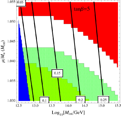
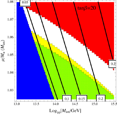
Figure 1: The Figures on the left and right show allowed regions (white) in the $\left[\hat{\mu}-\log(M_{\text{int}}/\text{GeV})\right]$ plane for $\tan\beta=5$ and $20$ respectively. In the red region the Higgs soft mass matrix does not have a negative eigenvalue and the vacuum is unstable in the blue region. The Higgs is lighter than 114 GeV in the green region, and the right-handed sleptons are lighter than the LEP bounds in the yellow region. In the yellow-green region both the Higgs and a slepton are lighter than their LEP bounds. The Higgs masses for these figures were computed in the decoupling limit [19]. Finally, the black contours lines are contours of $m_{A}/\mu$.

To visualize the allowed parameter space we choose two representative values for $\tan\beta$, $\tan\beta=5\text{ and }20$, and plot the parameter space as a function of the other two inputs, $\log(M_{\text{int}}/M_{\text{susy}})$ and $\hat{\mu}$ in Fig. 1. The allowed region is bounded by a number of constraints: i. one eigenvalue of the soft Higgs mass matrix must be negative so that electroweak symmetry breaking is triggered, $\left(m_{H_{u}}^{2}+|\mu|^{2}\right)\left(m_{H_{d}}^{2}+|\mu|^{2}\right)-|B_{\mu}|^{2}\;<\;0$, ii. vacuum stability requires $m_{H_{u}}^{2}+m_{H_{d}}^{2}+2|\mu|^{2}\;>\;2\>|B_{\mu}|$, iii. the Higgs mass bound from LEP $m_{h}>114$ GeV, iv. the bound on the mass of the right-handed sleptons $m_{\widetilde{e},\widetilde{\mu}}>100$ GeV and $m_{\widetilde{\tau}}>91$ GeV.

The remaining region in parameter space is quite constrained. Everywhere in parameter space we find $\hat{\mu}\gtrsim 1$ or $\mu\gtrsim M_{u}$. Furthermore we see that the intermediate scale is required to be quite high. This can be understood by looking at the renormalization group equation for the trace of the $H_{u}$-$H_{d}$ mass matrix which needs to be positive for vacuum stability but is driven negative by stop loops for small $M_{\text{int}}$. The plots we show here are for positive $\mu$, a similar region in parameter space is allowed for negative $\mu$.

As mentioned above $\mu$ is required to be quite large in order to obtain consistent electroweak symmetry breaking. This implies heavy Higgsinos. Usually in the MSSM large $\mu$ also implies large scalar Higgs masses and therefore large $m_{A}$. This is not the case in our scenario because of the cancellation between the soft mass $-|\mu|^{2}$ and supersymmetric mass $+|\mu|^{2}$ in the Higgs mass matrix. At the loop level,i.e. including running, the Higgs scalar mass matrix does not vanish but Higgs scalar masses remain much smaller than Higgsino masses. Hence we expect that the ratio of the pseudoscalar Higgs mass $m_{A}$ over Higgsino masses $\mu$ is small. This expectation is borne out by our numerical analysis as can be seen from the $m_{A}/\mu$ contours in Fig. 1.

	$\tan\beta$		$10$
Input	$\hat{\mu}$		$1.00$
	$M_{\text{int}}$		$10^{15}$ GeV
	$M_{1}$	$273$ GeV	$m_{Q_{1}}$	$1243$ GeV
	$M_{2}$	$510$ GeV	$m_{u_{1}}$	$1192$ GeV
	$M_{3}$	$1412$ GeV	$m_{d_{1}}$	$1186$ GeV
	$\mu$	$1246$ GeV	$m_{t_{1}}$	$1113$ GeV
	$B_{\mu}$	$\left(115~{}\text{GeV}\right)^{2}$	$m_{t_{2}}$	$1277$ GeV
Output	$m_{h}$	$115$ GeV	$m_{b_{1}}$	$1279$ GeV
	$m_{A}$	$365$ GeV	$m_{b_{2}}$	$1226$ GeV
	$m_{H^{0}}$	$377$ GeV	$m_{L_{1}}$	$389$ GeV
	$m_{H^{\pm}}$	$374$ GeV	$m_{E_{1}}$	$204$ GeV
	$a_{t}$	$-906$ GeV	$m_{\tau_{1}}$	$206$ GeV
			$m_{\tau_{2}}$	$397$ GeV

Table 1: A sample spectrum. We evaluated all soft masses at $M_{\text{susy}}=1~{}\text{TeV}$. Gauge couplings at $M_{\text{susy}}$ are derived from their $Z$-pole values using one-loop standard model RGEs. Yukawa couplings at $M_{\text{susy}}$ are derived from the running quark masses in the standard model at $1$ TeV [20]. All masses shown in the table are determined from the soft masses at one-loop level via tree level matching, except for the lightest neutral Higgs mass for which we included higher order corrections [21]. The MSSM soft parameters were run at one loop using [19], all soft masses are evaluated at $M_{\text{susy}}=1$ TeV.

We believe that this prediction, $m_{A}^{2}\ll|\mu|^{2}$, is unique to our scenario. A tell-tale signature which distinguishes our model from otherwise similar gaugino mediation models is therefore that charged Higgses $H^{\pm}$, the pseudoscalar Higgs $A^{0}$, and the heavy Higgs $H^{0}$ can all be produced directly or in cascade decays of stops and sbottoms with large cross sections at the LHC. On the other hand, Higgsinos are too heavy to be produced either directly or in cascades.

Another consequence of the negative Higgs soft masses at $M_{\text{int}}$ is that third generation scalar masses receive additional positive contributions from the running due to scalar Higgs loops. Consider for example the renormalization group equations for the soft masses squareds of staus. They contain a term proportional to $\lambda_{\tau}^{2}(m_{L_{3}}^{2}+m_{E_{3}}^{2}+m_{H_{d}}^{2})$. Since $M_{H_{d}}^{2}$ is negative and large this gives a positive contribution to the stau masses which is absent for smuons and selectrons because of the much smaller Yukawa couplings. One might still end up with a stau being the lightest slepton if there is large mixing between left- and right-handed staus. However the combination $m_{\tau_{1}}^{2}+m_{\tau_{2}}^{2}$ is independent of this mixing, and we predict that this is greater than $m_{L_{i}}^{2}+m_{E_{i}}^{2}$ for $i\in\{1,2\}$. Note that this predicted inequality is satisfied by the our example spectrum in Table 1. A similar argument applies to squarks. There the relevant combination $\lambda_{t}^{2}(m_{Q_{3}}^{2}+m_{U_{3}}^{2}+m_{H_{u}}^{2})$ starts out negative near $M_{\text{int}}$, however it turns positive because of the large squark masses generated from gaugino loops. Therefore we do not predict $m_{t_{1}}^{2}+m_{t_{2}}^{2}$ to be larger than the corresponding first and second generation squark masses squared. However we do expect $m_{t_{1}}^{2}+m_{t_{2}}^{2}$ larger than in usual MSSM spectra in which the contributions from negative Higgs soft masses are absent. For example, for the spectrum of Table 1 we have $m_{t_{1}}^{2}+m_{t_{2}}^{2}=(1694~{}\text{ GeV})^{2}$ to be compared with $m_{t_{1}}^{2}+m_{t_{2}}^{2}=(1535~{}\text{ GeV})^{2}$ which was obtained with the same boundary conditions at $M_{\text{int}}$ except that we set $m_{H_{u}}^{2}=m_{H_{d}}^{2}=0$.

We ran the MSSM masses at one loop using [19]. The masses quoted in Table. 1 are evaluated at $M_{\text{susy}}=1$ TeV.

Other features of our spectrum are shared with gaugino mediation [22]. For example, right-handed (charged) sleptons are the lightest MSSM superpartners [23, 24]. Obviously these cannot be the dark matter and the gravitino or an axion or another particle in addition to the MSSM may be the dark matter. Cascade decays in our model always end in right-handed sleptons. Depending on their lifetime, these may manifest themselves either as stable charged tracks or as displaced vertices from their decays to leptons and gravitinos [25, 26, 27].

4 Conclusions

In this paper we have shown that the scalar sequestering boundary condition with gaugino mass unification is compatible with radiative electroweak symmetry breaking, and that it produces a viable superpartner spectrum. Scalar sequestering drives all scalar masses to zero at an intermediate scale. Therefore any dependence of scalar masses on details of the messenger sector of supersymmetry breaking is removed by renormalization, and we find several messenger-model independent predictions for the superpartner spectrum. The running squark and slepton masses pass through zero at the intermediate scale when evolved with the MSSM renormalization group equations as in gaugino mediation. In addition, there are unique predictions which follow from the vanishing Higgs scalar mass matrix

$$\begin{pmatrix}m_{H_{u}}^{2}+|\mu|^{2}&B_{\mu}^{*}\\ B_{\mu}&m_{H_{d}}^{2}+|\mu|^{2}\end{pmatrix}=\begin{pmatrix}0&0\\ 0&0\end{pmatrix}\;.$$ (15)

These predictions are: Higgs scalars are much lighter than Higgsinos. Third generation sleptons (and to some extent also squarks, see the discussion near Table 3. for details) are lighter than their first and second generation counterparts due to the contributions from negative Higgs soft masses in the renormalization group equations.

We find the vanishing of the Higgs scalar mass matrix at $M_{\text{int}}$ also very intriguing from a theoretical point of view. It is interesting that supersymmetry breaking parameters $m_{H_{u}}^{2}$ and $m_{H_{d}}^{2}$ become related to the supersymmetry preserving parameter $\mu$ by hidden sector running. This is at least a partial solution to the $\mu$-problem once one realizes that the $\mu$ problem may be formulated as the need for an explanation for why the combinations $m_{H_{u}}^{2}+|\mu|^{2}$ and $m_{H_{d}}^{2}+|\mu|^{2}$ are small compared to $m_{H_{u}}^{2}$, $m_{H_{d}}^{2}$ and $|\mu^{2}|$ individually.

In this paper we minimized the number of free parameters by making the additional assumption of gaugino mass unification. We found that the allowed region in parameter space is very small, leading to very specific predictions for the spectrum. Clearly, if one allows the gaugino masses to vary independently, it becomes much easier to find solutions to the electroweak symmetry breaking conditions. We believe that such models might have very low levels of fine tuning in the Higgs sector.

Finally, we wish to comment on the recent paper Ref. [28] which has some overlap with our work. The authors of Ref. [28] assumed the relationship $|\mu^{2}|=|a_{t}a_{b}|$ which follows from specific assumptions about the couplings of $H_{u}$ and $H_{d}$ to the messenger sector. With this additional constraint they found no solutions to the electroweak symmetry breaking conditions Eqs. (12) and (13). To avoid this problem, the authors of [28] introduced additional free parameters for the gaugino masses. In our paper we did not make any assumptions about the relationship between $\mu$ and the $A$-terms because such relationships are messenger-model dependent. We found that then there are solutions to the electroweak symmetry breaking conditions without the need to give up gaugino mass unification.

Appendix A The proof

We wish to prove Eq. (9), i.e. that the coefficients of the Higgs soft mass operators run to fixed point values equal to minus the square of the coefficient of the $\mu$-term operators. Our context is the MSSM coupled to an approximately conformal hidden sector through higher-dimensional operators. We also assume that the hidden sector couplings are sufficiently large so that their effects dominate over any running due to MSSM couplings, and it is a good approximation to ignore the MSSM couplings.

As a warm-up let us first discuss the renormalization of the Higgs soft masses in absence of the $\mu$ and the $B_{\mu}$ term operators but with the most general coupling between the hidden and visible sectors. Since we are ignoring visible sector interactions it suffices to look at a single chiral superfield of the visible sector $H$ coupled to hidden sector operators $\mathcal{X}$ and $\mathcal{R}$

$$\int\!\!\!d^{4}\theta\ H^{\dagger}\!H\>(1+x\,\frac{\mathcal{X}}{M_{*}}+x^{\dagger}\,\frac{\mathcal{X^{\dagger}}}{M_{*}}+x^{\dagger}x\,\frac{\mathcal{X^{\dagger}X}}{M_{*}^{2}}+r\frac{\mathcal{R}}{M_{*}^{2}})+\mathcal{L}_{\text{hidden}}\;.$$ (16)

We assumed that operators with derivatives are less relevant so that we can ignore them. The chiral operator $\mathcal{X}$ may actually consist of a sum of terms so that $x$ is a complex vector of coefficients. The operator $\mathcal{R}$ is real and the corresponding coefficient vector $r$ is real as well. Note that we could have absorbed the term proportional to $x^{\dagger}x$ by an appropriate shift in $r$ but we will see that separating the operators in this way is preferable.

The easiest way to understand the renormalization of the scalar mass operators is to first redefine fields to remove the chiral couplings of $\mathcal{X}$ to $H^{\dagger}H$. To do so we define

$$\tilde{H}\equiv(1+x\,\frac{\mathcal{X}}{M_{*}})H\;.$$ (17)

Ignoring operators of order $(\frac{\mathcal{X}}{M_{*}})^{3}$ or higher our Lagrangian becomes

$$\int\!\!\!d^{4}\theta\ \tilde{H}^{\dagger}\!\tilde{H}\>(1+r\,\frac{\mathcal{R}}{M_{*}^{2}})+\mathcal{L}_{\text{hidden}}\ ,$$ (18)

and all dependence on $x$ has disappeared, this was the reason for splitting out the $x^{\dagger}x$ term from $r$ in Eq. (16). Since the Lagrangian is independent of $x$ it is clear that the running of operator coefficients $r$ is independent of $x$ and $\mathcal{X}$, and also the scalar masses are independent of $x$ and $\mathcal{X}$.

We now assume that our hidden sector is a strongly coupled approximately conformal field theory so that the running of operator coefficients can be approximated by anomalous dimensions. We further assume that the anomalous dimensions ${\gamma_{\mathcal{R}}}$ of the real operators $\mathcal{R}$ are positive. This is a strong assumption but given the large number of approximately conformal field theories which we can construct we believe that it is a reasonable assumption that hidden sectors with the desired properties exist [10]. The renormalization group equation for the coefficients $r$ is then (the Feynman diagrams which contribute are of the form of the third diagram in Figure 2.)

$$\frac{d\,r}{dt}={\gamma_{\mathcal{R}}}\,r$$ (19)

with the low energy solution

$$r\,\Big{|}_{M_{\text{int}}}\>=\>\left(\frac{M_{\text{int}}}{M_{*}}\right)^{\gamma_{\mathcal{R}}}\>r\,\Big{|}_{M_{*}}\ .$$ (20)

Thus the resulting scalar masses squared are suppressed by the factor $(M_{\text{int}}/M_{*})^{{\gamma_{\mathcal{R}}}}$ relative to the gaugino masses which have no such suppression. i.e. the scalar masses are sequestered.

figure1 (20,20) b1,b2t1 shaded,smooth,pull=1.8,tension=0.8H3 phantomb1,v1,H1 phantomH2,v2,b2 phantom,tension=2t1,H3 double,label=$\mathcal{X}$,l.side=left,left=0.2v1,H1 double,label=$\mathcal{X}^{\dagger}$,l.side=left,left=0.2H2,v2 dbl_wiggly,label=$\mathcal{R}$,tension=2H3,t1 phantom_arrow,left=0.2v1,H1 phantom_arrow,left=0.2H2,v2 fermion,label=$H^{\dagger}$,l.side=leftb1,v1 fermion,label=$H$,l.side=rightv1,v2 fermion,label=$H$,l.side=leftv2,b2 v2 (20,20) b1,b2t1 shaded,smooth,pull=1.8,tension=0.5H3 phantomb1,v1,H1 phantomH2,v1,b2 phantom,tension=2.5t1,H3 double,label= $\mathcal{X}$,l.side=left,left=0.4v1,H1 double,label=$\!\!\!\mathcal{X}^{\dagger}$,l.side=left,left=0.4H2,v1 dbl_wiggly,label=$\mathcal{R}$,tension=2H3,t1 phantom_arrow,left=0.4v1,H1 phantom_arrow,left=0.4H2,v1 fermion,label=$H^{\dagger}$ ,l.side=leftb1,v1 fermion,label=$\ H$,l.side=leftv1,b2 v1 (20,20) i1,o1 t1 fermion,label=$H^{\dagger}$,l.side=lefti1,v1 fermion,label=$H$,l.side=leftv1,o1 dbl_wiggly,label=$\mathcal{R}$,l.side=left,tension=2t1,v2 dbl_wiggly,label=$\mathcal{R}$,l.side=left,tension=2v2,v1 v2 .3wv2

Figure 2: Renormalization of the Higgs soft mass operators $\mathcal{R}H^{\dagger}H$ due to the operators $\left(\mathcal{X}+\mathcal{X}^{\dagger}\right)H^{\dagger}H$, $\mathcal{X^{\dagger}X}H^{\dagger}H$ and $\mathcal{R}H^{\dagger}H$ itself.

Note that we could have derived the same result without performing the field redefinition of Eq. (17). In this basis the renormalization is slightly more complicated because the operators $\frac{\mathcal{X}}{M_{*}}H^{\dagger}H$ and $\frac{\mathcal{X^{\dagger}\!X}}{M_{*}^{2}}H^{\dagger}H$ now also contribute to the renormalization of $r$ via the two left-most diagrams in Fig. 2. Note that the “blobs” in these two diagrams represent identical hidden sector interactions. Therefore the diagrams are proportional to identical unknown hidden sector factors. But the first diagram is proportional to $(-ix)^{\dagger}i(-ix)=+ix^{\dagger}x$ from the two vertices and the “propagator” for the F-component of $H$, whereas the second diagram has a $-ix^{\dagger}x$ from the vertex. Therefore the two diagrams cancel, and the renormalization group equation for $r$ only receives contributions from the third diagram in Fig. 2. Thus we see that the running of $r$ is the same as in the other basis, and $r$ is suppressed by $(M_{\text{int}}/M_{*})^{\gamma_{\mathcal{R}}}$ in the infrared. Note that the $x$-dependent part of the Lagrangian does not run (the term linear in $x$ is protected by the non-renormalization theorem, and the coefficient $x^{\dagger}x$ is equal to the square of the linear $x$ coefficient by definition). At $M_{\text{int}}$ the $r$ terms can be neglected, and the remaining Lagrangian is

$$\int\!\!\!d^{4}\theta\ H^{\dagger}\!H\>\left(1+x\,\frac{\mathcal{X}}{M_{*}}+x^{\dagger}\,\frac{\mathcal{X^{\dagger}}}{M_{*}}+x^{\dagger}x\,\frac{\mathcal{X^{\dagger}\!X}}{M_{*}^{2}}\right)+\>\mathcal{L}_{\text{hidden}}\ .$$ (21)

This Lagrangian does not give $H$ scalar masses because the contributions from $F$-terms in $\frac{\mathcal{X}}{M_{*}}$ cancel the masses from $D$-terms in $\frac{\mathcal{X^{\dagger}\!X}}{M_{*}^{2}}$. This can be seen explicitly by integrating out the auxiliary components of $H$ or - more easily - by performing the redefinition to $\tilde{H}$ fields.

This completes our study of the renormalization of the Higgs soft mass in the presence of the coupling $\frac{\mathcal{X}}{M_{*}}H^{\dagger}H$, but without the operators responsible for generating the $\mu$ and $B_{\mu}$ terms. The reason for considering this simpler case first is that the running of the Higgs soft mass operators ($\frac{\mathcal{X}^{\dagger}\mathcal{X}}{M_{*}^{2}}H^{\dagger}H$) due to the $\mu$-term operator can be understood by performing a similar field redefinition to the one given in Eq. (17). We now turn to our proof in the general case which includes the $\mu$-operator $\frac{\mathcal{X}^{\dagger}}{M_{*}}H_{u}H_{d}$.

Ignoring any (weak) visible sector interactions the relevant Lagrangian which couples $H_{u}$, $H_{d}$ to the hidden sector fields is

$$\int\!\!\!d^{4}\theta\ \Bigg{[}H_{u}^{\dagger}H_{u}+H_{d}^{\dagger}H_{d}+x_{\mu}^{\dagger}\>\frac{\mathcal{X}}{M_{*}}H_{d}^{\dagger}H_{u}^{\dagger}+x_{\mu}\!\frac{\mathcal{X^{\dagger}}}{M_{*}}H_{u}H_{d}+r_{u}\>\frac{\mathcal{R}}{M_{*}^{2}}H_{u}^{\dagger}H_{u}+r_{d}\>\frac{\mathcal{R}}{M_{*}^{2}}H_{d}^{\dagger}H_{d}\Bigg{]}\ .$$ (22)

Note that we have written the Lagrangian directly in the basis for $H_{u}$ and $H_{d}$ in which there are no chiral $\mathcal{X}$ couplings to $H_{u}^{\dagger}H_{u}$ and $H_{d}^{\dagger}H_{d}$. There is also the operator $\mathcal{R}H_{u}H_{d}$ which contributes to $B_{\mu}$. This operator scales to zero in the infrared because of the anomalous dimension of $\mathcal{R}$ which explains why $B_{\mu}\simeq 0$ at $M_{\text{int}}$. Since $\mathcal{R}H_{u}H_{d}$ does not contribute to the renormalization of the soft masses $m_{H_{u}}^{2}$ and $m_{H_{d}}^{2}$ we have not included it in Eq. (22).

figure2 (20,20) b1,b2t1 shaded,smooth,pull=1.8,tension=0.8H3 phantomb1,v1,H1 phantomH2,v2,b2 phantom,tension=2t1,H3 double,label=$\mathcal{X}$,l.side=left,left=0.2v1,H1 double,label=$\mathcal{X}^{\dagger}$,l.side=left,left=0.2H2,v2 dbl_wiggly,label=$\mathcal{R}$,tension=2H3,t1 phantom_arrow,left=0.2v1,H1 phantom_arrow,left=0.2H2,v2 fermion,label=$H_{u}^{\dagger}$,l.side=leftb1,v1 fermion,label=$H_{d}$,l.side=leftv2,v1 fermion,label=$H_{u}$,l.side=leftv2,b2 v2 (20,20) b1,b2t1 shaded,smooth,pull=1.8,tension=0.5H3 phantomb1,v1,H1 phantomH2,v1,b2 phantom,tension=2.5t1,H3 double,label= $\mathcal{X}$,l.side=left,left=0.4v1,H1 double,label=$\!\!\!\mathcal{X}^{\dagger}$,l.side=left,left=0.4H2,v1 dbl_wiggly,label=$\mathcal{R}$,tension=2H3,t1 phantom_arrow,left=0.4v1,H1 phantom_arrow,left=0.4H2,v1 fermion,label=$H_{u}^{\dagger}$ ,l.side=leftb1,v1 fermion,label=$\ H_{u}$,l.side=leftv1,b2 v1 (20,20) i1,o1 t1 fermion,label=$H_{u}^{\dagger}$,l.side=lefti1,v1 fermion,label=$H_{u}$,l.side=leftv1,o1 dbl_wiggly,label=$\mathcal{R}$,l.side=left,tension=2t1,v2 dbl_wiggly,label=$\mathcal{R}$,l.side=left,tension=2v2,v1 v2 .3wv2

Figure 3: Renormalization of the Higgs soft mass operators $\mathcal{R}H_{u}^{\dagger}H_{u}$. The left-most diagram is due to the $\mu$-operator $\mathcal{X}^{\dagger}H_{u}H_{d}$.

Let us first consider renormalization of the $H_{u}$ mass. The diagrams which contribute are the first and third diagrams from left in Fig. 3 (according to our definition of the Lagrangian in Eq. (22)). Note that neither of the two diagrams involves an internal $H_{u}$ line. Thus for the purpose of computing the $H_{u}$ mass we may treat $H_{u}$ as a non-propagating background field. Furthermore, we can drop all components of $H_{u}$ except for the scalar. Finally we can even set the scalar component of $H_{u}$ equal to a constant. Our goal will be to compute the dependence of the low energy effective Lagrangian on this complex doublet of numbers $H_{u}$ Our goal will be to compute the dependence of the low energy effective Lagrangian on $H_{u}$. The full $H_{u}$ scalar mass (i.e. the $(1,1)$ entry of the matrix in Eq. (1) which consist of both the SUSY and the non-SUSY contributions) is simply the coefficient of $H_{u}^{\dagger}H_{u}$ in this Lagrangian. Eq. (22) can be rewritten as

$$\int\!\!\!d^{4}\theta\ \Bigg{[}\left(H_{d}^{\dagger}+x_{\mu}\,\frac{\mathcal{X^{\dagger}}}{M_{*}}H_{u}\right)\left(H_{d}+x_{\mu}^{\dagger}\,\frac{\mathcal{X}}{M_{*}}H_{u}^{\dagger}\right)+\left(r_{u}\,\frac{\mathcal{R}}{M_{*}^{2}}-x_{\mu}^{\dagger}x_{\mu}\,\frac{\mathcal{X^{\dagger}\!X}}{M_{*}^{2}}\right)\!\>H_{u}^{\dagger}H_{u}\Bigg{]}\ .$$ (23)

Note that there is no kinetic term for the number $H_{u}$, we have dropped the operator $\mathcal{R}H_{d}^{\dagger}H_{d}$ because it does not contribute to the renormalization of the $H_{u}$ mass, and we have grouped the $H_{d}$ kinetic term and the bosonic part of the $\mu$-operator together by completing the square. In order to bring this to a form similar to Eq. (16), we redefine the vector of coefficients $r_{u}$

$$\tilde{r}_{u}\equiv r_{u}-x_{\mu}^{\dagger}x_{\mu}\;,$$ (24)

so that our Lagrangian becomes

$$\int\!\!\!d^{4}\theta\ \Bigg{[}\left(H_{d}^{\dagger}+x_{\mu}\,\frac{\mathcal{X^{\dagger}}}{M_{*}}H_{u}\right)\left(H_{d}+x_{\mu}^{\dagger}\,\frac{\mathcal{X}}{M_{*}}H_{u}^{\dagger}\right)+\tilde{r}_{u}\,\frac{\mathcal{R}}{M_{*}^{2}}H_{u}^{\dagger}H_{u}\Bigg{]}\;.$$ (25)

The $r_{u}$ redefinition can absorb the couplings of $\mathcal{X^{\dagger}X}$ to $H_{u}^{\dagger}H_{u}$ because the vector of real operators $\mathcal{R}$ contains all possible operators of the form $\mathcal{X^{\dagger}X}$. In this basis there is now a one to one correspondence between the terms in Eq. (25) and the terms in Eq. (16). We will exploit this correspondence when we discuss the diagrammatic proof at the end of this Section.

But let us first understand the proof using a field redefinition. We define

$$\tilde{H}_{d}\equiv H_{d}+x_{\mu}^{\dagger}\,\frac{\mathcal{X}}{M_{*}}\>H_{u}^{\dagger}\ ,$$ (26)

and our Lagrangian reduces to

$$\int\!\!\!d^{4}\theta\ \Bigg{[}\tilde{H}_{d}^{\dagger}\tilde{H}_{d}+\tilde{r}_{u}\,\frac{\mathcal{R}}{M_{*}^{2}}H_{u}^{\dagger}H_{u}\Bigg{]}\;.$$ (27)

This field redefinition preserves supersymmetry despite the daggers in it’s definition. The key is that $H_{u}^{\dagger}$ is not a full anti-chiral superfield, it is simply a doublet of complex numbers. The $\mathcal{X}$ appearing in the field redefinition is chiral which is important because both $\mathcal{X}$ and $H_{d}$ are dynamical and we do not want to destroy manifest supersymmetry by mixing up chiral and anti-chiral fields.

In this new basis things have become very simple. $\tilde{H}_{d}$ has completely decoupled and does not contribute to the renormalization of the $H_{u}$ mass. The scaling of $\tilde{r}_{u}$ entirely comes from the anomalous dimension of $\mathcal{R}$ (the third diagram in Fig. 3.) Thus

$$\tilde{r}_{u}\,\Big{|}_{M_{\text{int}}}\>=\>\left(\frac{M_{\text{int}}}{M_{*}}\right)^{\gamma_{\mathcal{R}}}\,\tilde{r}_{u}\,\Big{|}_{M_{*}}\;.$$ (28)

which tends to zero as $M_{\text{int}}\ll M_{*}$ because ${\gamma_{\mathcal{R}}}>0$. Now we can read off the $H_{u}$ scalar mass at $M_{\text{int}}$. It is

$$\left(\frac{M_{\text{int}}}{M_{*}}\right)^{\gamma_{\mathcal{R}}}\>\tilde{r}_{u}(M_{*})\>\frac{D}{M_{*}^{2}}\quad\sim\left(\frac{M_{\text{int}}}{M_{*}}\right)^{\gamma_{\mathcal{R}}}M_{\text{SUSY}}^{2}$$ (29)

which is negligibly small compared to $M_{\text{SUSY}}^{2}$, the mass scale of the gaugino masses. Let us emphasize that this is the full scalar mass which includes both the contribution from the $\mu$ term as well as from soft supersymmetry breaking.

We can also extract the soft supersymmetry breaking mass $m_{H_{u}}^{2}$ by undoing the field redefinition Eq. (26) at the scale $M_{\text{int}}$ to obtain the low-energy Lagrangian (we have set $\tilde{r}_{u}(M_{\text{int}})=0$)

$$\begin{split}\int\!\!\!d^{4}\theta\>&\left(H_{d}^{\dagger}+x_{\mu}\,\frac{\mathcal{X^{\dagger}}}{M_{*}}H_{u}\right)\left(H_{d}+x_{\mu}^{\dagger}\,\frac{\mathcal{X}}{M_{*}}H_{u}^{\dagger}\right)\\ =&\int\!\!\!d^{4}\theta\ \Bigg{[}H_{d}^{\dagger}H_{d}+x_{\mu}^{\dagger}\,\frac{\mathcal{X}}{M_{*}}H_{d}^{\dagger}H_{u}^{\dagger}+x_{\mu}\,\frac{\mathcal{X^{\dagger}}}{M_{*}}H_{u}H_{d}+x_{\mu}^{\dagger}x_{\mu}\,\frac{\mathcal{X^{\dagger}\!X}}{M_{*}^{2}}H_{u}^{\dagger}H_{u}\Bigg{]}\;.\end{split}$$ (30)

Here the term proportional to $\mathcal{X}$ is the $\mu$-operator which contributes $+|\mu|^{2}$ to the $H_{u}$ scalar mass and the term proportional to $\mathcal{X^{\dagger}X}$ is the soft mass squared. It is equal to

$$m_{H_{u}}^{2}=-\>x_{\mu}^{\dagger}x_{\mu}\frac{\mathcal{X^{\dagger}\!X}}{M_{*}^{2}}\Big{|}_{D}\>=-|\mu|^{2}\;.$$ (31)

Of course, with a completely analogous argument we may compute the $H_{d}$ mass and find

$$m_{H_{d}}^{2}=m_{H_{u}}^{2}=-|\mu|^{2}\ ,$$ (32)

which is what we set out to prove.

Alternatively, we can also construct a diagrammatic proof without making use of the field redefinition of Eq. 26. The proof is completely analogous to the diagrammatic proof considered at the beginning of the Appendix. Our starting point is the Lagrangian Eq. (25), which leads to the Feynman diagrams in Fig. 3. As before, the two left-most diagrams in the Figure have identical blobs and give canceling contributions to the renormalization of $\tilde{r}_{u}$. The third diagram gives

$$\frac{d\,\tilde{r}_{u}}{dt}={\gamma_{\mathcal{R}}}\,\tilde{r}_{u}\;.$$ (33)

For positive ${\gamma_{\mathcal{R}}}$ this equation has an attractive infrared fixed point at which $\tilde{r}_{u}=0$. And undoing the shift Eq. (24) we obtain $\left|r_{u}\right|_{M_{\text{int}}}=\left.x_{\mu}^{\dagger}x_{\mu}\right|_{M_{\text{int}}}$, and therefore $m_{H_{u}}^{2}=-|\mu|^{2}$.

References

- [1] M. A. Luty and R. Sundrum, Phys. Rev. D 65, 066004 (2002) [arXiv:hep-th/0105137].
- [2] M. Luty and R. Sundrum, Phys. Rev. D 67, 045007 (2003) [arXiv:hep-th/0111231].
- [3] M. Dine, P. J. Fox, E. Gorbatov, Y. Shadmi, Y. Shirman and S. D. Thomas, Phys. Rev. D 70, 045023 (2004) [arXiv:hep-ph/0405159].
- [4] M. Ibe, K. I. Izawa, Y. Nakayama, Y. Shinbara and T. Yanagida, Phys. Rev. D 73, 015004 (2006) [arXiv:hep-ph/0506023].
- [5] M. Ibe, K. I. Izawa, Y. Nakayama, Y. Shinbara and T. Yanagida, Phys. Rev. D 73, 035012 (2006) [arXiv:hep-ph/0509229].
- [6] M. Schmaltz and R. Sundrum, JHEP 0611, 011 (2006) [arXiv:hep-th/0608051].
- [7] A. G. Cohen, T. S. Roy and M. Schmaltz, JHEP 0702, 027 (2007) [arXiv:hep-ph/0612100].
- [8] Y. Kawamura, T. Kinami and T. Miura, arXiv:0810.3965 [hep-ph].
- [9] B. A. Campbell, J. Ellis and D. W. Maybury, arXiv:0810.4877 [hep-ph].
- [10] T. S. Roy and M. Schmaltz, Phys. Rev. D 77, 095008 (2008) [arXiv:0708.3593 [hep-ph]].
- [11] H. Murayama, Y. Nomura and D. Poland, Phys. Rev. D 77, 015005 (2008) [arXiv:0709.0775 [hep-ph]].
- [12] D. E. Kaplan, G. D. Kribs and M. Schmaltz, Phys. Rev. D 62, 035010 (2000) [arXiv:hep-ph/9911293].
- [13] Z. Chacko, M. A. Luty, A. E. Nelson and E. Ponton, JHEP 0001, 003 (2000) [arXiv:hep-ph/9911323].
- [14] C. Csaki, J. Erlich, C. Grojean and G. D. Kribs, Phys. Rev. D 65, 015003 (2002) [arXiv:hep-ph/0106044].
- [15] H. C. Cheng, D. E. Kaplan, M. Schmaltz and W. Skiba, Phys. Lett. B 515, 395 (2001) [arXiv:hep-ph/0106098].
- [16] G. R. Dvali, G. F. Giudice and A. Pomarol, Nucl. Phys. B 478, 31 (1996) [arXiv:hep-ph/9603238].
- [17] M. Yamaguchi and K. Yoshioka, Phys. Lett. B 543, 189 (2002) [arXiv:hep-ph/0204293].
- [18] G. F. Giudice, H. D. Kim and R. Rattazzi, Phys. Lett. B 660, 545 (2008) [arXiv:0711.4448 [hep-ph]].
- [19] S. P. Martin, arXiv:hep-ph/9709356.
- [20] Z. z. Xing, H. Zhang and S. Zhou, Phys. Rev. D 77, 113016 (2008) [arXiv:0712.1419 [hep-ph]].
- [21] A. Djouadi, J. L. Kneur and G. Moultaka, Comput. Phys. Commun. 176, 426 (2007) [arXiv:hep-ph/0211331].
- [22] M. Schmaltz and W. Skiba, Phys. Rev. D 62, 095004 (2000) [arXiv:hep-ph/0004210].
- [23] S. Dimopoulos, M. Dine, S. Raby and S. D. Thomas, Phys. Rev. Lett. 76, 3494 (1996) [arXiv:hep-ph/9601367].
- [24] S. Dimopoulos, M. Dine, S. Raby, S. D. Thomas and J. D. Wells, Nucl. Phys. Proc. Suppl. 52A, 38 (1997) [arXiv:hep-ph/9607450].
- [25] P. Fayet, Phys. Lett. B 70, 461 (1977).
- [26] P. Fayet, Phys. Lett. B 84, 416 (1979).
- [27] R. Casalbuoni, S. De Curtis, D. Dominici, F. Feruglio and R. Gatto, Phys. Lett. B 215, 313 (1988).
- [28] M. Asano, J. Hisano, T. Okada and S. Sugiyama, arXiv:0810.4606 [hep-ph].