Parallel magnetic field tuning of valley splitting in AlAs two-dimensional electrons

Abstract

We demonstrate that, in a quasi-two-dimensional electron system confined to an AlAs quantum well and occupying two conduction-band minima (valleys), a parallel magnetic field can couple to the electrons’ orbital motion and tune the energies of the two valleys by different amounts. The measured density imbalance between the two valleys, which is a measure of the valley susceptibility with respect to parallel magnetic field, is enhanced compared to the predictions of non-interacting calculations, reflecting the role of electron-electron interaction.

The physics governing the valley splitting in multi-valley two-dimensional electron systems (2DESs), such as in Si field-effect-transistors, has been of interest for some time Dorda78PRB ; Ando82RevModPhys . It is attracting renewed attention in 2DESs in Si, AlAs, and graphene Eng07PRL ; Geim2007Nature , both as a fundamental problem, and also because of the possibility that manipulating the electron valley degree of freedom might lead to novel (”valleytronics”) devices Gunawan2007PRB ; Gunawan2008PRL ; Rycerz2007Nature . Traditionally, the valley energies have been controlled via strain, confinement and electric field Dorda78PRB ; Ando82RevModPhys ; Takashina2004PRB ; ShkolnikovFootnote . In this Letter we demonstrate how a magnetic field ($B_{\parallel}$) applied $parallel$ to the 2D plane can also break the valley degeneracy and shift the valley energies of a 2DES with finite layer thickness. In such a system, $B_{\parallel}$ couples to the electron orbital motion and deforms the electron wave function in the confinement direction. To first order, this deformation increases the valley energies (diamagnetic shift) and, to second order, it increases the effective mass in the direction perpendicular to $B_{\parallel}$ Batke87PRB ; Kunze87PRB ; Stern67 ; Stern68 ; Tutuc03PRB . In our AlAs samples, where two valleys with anisotropic Fermi contours are occupied, when $B_{\parallel}$ is applied along the major axis of one the valleys and perpendicular to the other valleys’ major axis, it shifts the valleys’ energies by different amounts. Remarkably, the measured energy shift and the resulting valley density imbalance are much larger than simple calculations would predict, signaling a clear enhancement of the $B_{\parallel}$-induced valley spitting, likely due to electron-electron interaction. (The parameter $r_{s}$, defined as the average inter-electron spacing measured in units of the effective Bohr radius, ranges from 6.4 to 9.8 for our samples.)

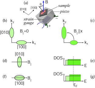
Figure 1: (Color online) Schematic diagrams showing: (a) Experimental setup; (b) and (c) Valley occupations at zero (light green) and finite (dark green) parallel magnetic fields; (d) and (f) Fermi contour distortions due to parallel magnetic field for the [100] and [010] valleys; (e) and (g) Density-of-states (DOS) for the [100] and [010] valleys before (light green) and after (dark green) the application of parallel magnetic field.

Figure 1 summarizes our experimental setup and measurements. We studied four samples; here we focus on two samples where the 2DES is confined to either an 11 nm-wide or a 15 nm-wide AlAs quantum well (QW), grown using molecular beam epitaxy on a semi-insulating GaAs (001) substrate. The AlAs well is flanked by AlGaAs barriers and is modulation-doped with Si PoortereAPL2002 . In these samples the electrons occupy two conduction-band valleys with elliptical Fermi contours as shown in Fig. 1(b) ShayeganPSS2006 , each centered at an X point of the Brillouin zone, and with an anisotropic effective mass (longitudinal mass $m_{l}=1.05$ and transverse mass $m_{t}=0.20$, in units of free electron mass, $m_{e}$) Gunawan2007PRB . We denote these two valleys according to the direction of their major axis: [100] and [010] (Fig. 1(b)). In our experiments $B_{\parallel}$ is applied along [100] as schematically shown in Fig. 1(a). Since the two valleys have different orientations with respect to $B_{\parallel}$, the diamagnetic shift and the effective mass enhancement are different for the two valleys, as illustrated in Figs. 1(d-g), causing an electron transfer from the [100] to the [010] valley (see Fig. 1(c)). This density imbalance ($\Delta n$) caused by $B_{\parallel}$ can be countered by applying symmetry-breaking strain $\epsilon=\epsilon_{[100]}-\epsilon_{[010]}$, where $\epsilon_{[100]}$ and $\epsilon_{[010]}$ are the strain values along the [100] and [010] directions. In our study, we monitored the sample resistance vs. $\epsilon$ at different values of $B_{\parallel}$ to determine $\Delta n$ as a function of $B_{\parallel}$. In order to apply tunable strain our samples were glued to a piezoelectric stack actuator as shown in Fig. 1(a) ShayeganPSS2006 ; GunawanPRL2006 . The measurements were performed in a ³He cryostat with a base temperature of 0.3 K. The system was equipped with a tilting stage, allowing the angle $\theta$ between the sample normal and the magnetic field to be varied in situ.

Before presenting the experimental data, we will first outline the theoretical formalism that describes this valley splitting. Using the same approach as in Refs. Stern67 and Stern68 , we start with a simple, single-particle effective mass Hamiltonian in three-dimensions:

$$H_{3D}=\frac{p_{x}^{2}}{2m_{x}}+\frac{(p_{y}+qB_{\parallel}z)^{2}}{2m_{y}}+\frac{p_{z}^{2}}{2m_{z}}+V(z)$$

where $p_{x}$, $p_{y}$, $p_{z}$ are momentum operators, $m_{x}$, $m_{y}$, $m_{z}$ are effective masses in $x$, $y$, $z$ directions, $q$ is the electron charge and $V(z)$ is the confinement potential in the $z$ direction which is assumed to be a QW with 210 meV barrier heights and 11 nm or 15 nm of well width for our two sample structures ShayeganPSS2006 . We use the gauge $\vec{A}=(0,B_{\parallel}z,0)$. Solutions to the above Hamiltonian are plane waves in $x$ and $y$ directions. Substituting the plane wave solutions leads to the one-dimensional Hamiltonian:

$$H_{1D}=\frac{p_{z}^{2}}{2m_{z}}+V(z)+\frac{2\hbar k_{y}qB_{\parallel}z+(qB_{\parallel}z)^{2}}{2m_{y}}$$

where the last two terms containing $B_{\parallel}$ can be described as perturbations to the Hamiltonian $H_{0}=p_{z}^{2}/2m_{z}+V(z)$. To first order, the ground state energy is shifted to higher values because of the second perturbation term, $(qB_{\parallel}z)^{2}/2m_{y}$. To second order, the effective mass in the $y$ direction ($\hbar^{2}/(d^{2}E/dk_{y}^{2})$) becomes enhanced since the first perturbation term ($\hbar k_{y}qB_{\parallel}z/m_{y}$) is linear with $k_{y}$. Eventually, the total energy for the ground state can be written as follows:

$$E=\frac{\hbar^{2}k_{x}^{2}}{2m_{x}}+\frac{\hbar^{2}k_{y}^{2}}{2m_{y}^{{}^{\prime}}}+E_{0}+\Delta E_{0}$$

where $E_{0}$ is the ground state energy of $H_{0}$, $\Delta E_{0}$ is the ground state energy shift, and $m_{y}^{{}^{\prime}}$ is the enhanced effective mass in the $y$ direction.

Initially, the two valleys have the same solutions to $H_{0}$ because of their same mass in the $z$ direction. The crucial observation is that the perturbation terms in Eq. (2) depend on $m_{y}$ which is different for the two valleys. The [100] valley has a smaller mass in the $y$ direction and therefore feels a stronger perturbation at a given $B_{\parallel}$. Its energy is shifted more compared to the [010] valley, causing a splitting with $B_{\parallel}$. The quantity we measure experimentally is $\Delta n$ caused by $B_{\parallel}$, and contains two terms: one, the difference in the ground state energies and the other, the difference in the density-of-states caused by the mass enhancement. To second order in perturbation, $\Delta n$ can be written as:

$$\Delta n=\alpha(\frac{1}{m_{l}}-\frac{1}{m_{t}})(1-\frac{2\pi\hbar^{2}n}{(E_{1}-E_{0})\sqrt{m_{l}m_{t}}})\frac{\sqrt{m_{l}m_{t}}}{2\pi\hbar^{2}}$$

where $\alpha=(1/2)q^{2}B_{\|}^{2}(\langle z^{2}\rangle-\langle z\rangle^{2})$ and $E_{1}$ is the first excited state energy of $H_{0}$. Although second order perturbation theory gives analytic answers, in our calculations we numerically solved the Schrodinger’s equation using a finite difference method; i.e., the values we report are numerically exact solutions to $H_{1D}$ in Eq. (2).

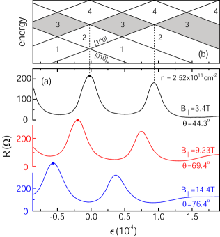
Figure 2: (Color online) (a) Resistance vs. strain traces for an 11 nm-wide AlAs QW taken at $\nu=3$ for different parallel magnetic fields. The ”balanced point” for a given $B_{\parallel}$ is marked by a closed circle on the corresponding trace. (b) Landau level fan diagram for $B_{\parallel}=3.4$ T as a function of $\epsilon$.

Experimentally, we determine $\Delta n$ vs. $B_{\parallel}$ by monitoring the sample resistance ($R$) as a function of $\epsilon$ in tilted magnetic fields. Examples of such piezo-resistance traces are shown in Fig. 2(a). Each trace was taken at a fixed $\theta$ and magnetic field so that the 2DES remains at a fixed Landau level (LL) filling factor ($\nu$=3 in the case of Fig. 2(a) data). With applied $\epsilon$, the LLs for the [100] and [010] valleys cross each other, as the fan diagram in Fig. 2(b) indicates. $R$ exhibits minima as the Fermi energy ($E_{F}$) passes through consecutive energy gaps, and maxima as it coincides with the LL crossings. The fan diagram in Fig. 2(b) is drawn for a fully spin polarized system; this is indeed the case for the traces shown in Fig. 2(a) because of the large Zeeman splitting due to the high magnetic field. From the piezo-resistance traces, the ”balanced point,” i.e., the strain at which the valleys are equally occupied at a given $B_{\parallel}$ can be measured by following the resistance peaks indicated by closed circles. (The balanced point at $B_{\parallel}=0$, which corresponds to $\epsilon=0$, is determined experimentally from $R$ vs. $\epsilon$ sweeps at even fillings as has been detailed in Ref. GunawanPRL2006 .) The data of Fig. 2 clearly show that the valley energies are split with the application of $B_{\parallel}$.

In Fig. 3(a) we show a set of $R$ vs. $\epsilon$ traces taken at a fixed $\theta$ for $\nu=$ 4, 5 and 6. Again, in all these traces, the 2DES is fully spin polarized because of the very large $B_{\parallel}$. The traces are periodic in $\epsilon$, implying that they are consistent with a simple, linear LL fan diagram, an example of which is shown in Fig. 6(b) for $\nu=6$. By associating the $R$ maxima with the LL coincidences, we can determine the valley polarization, $P_{V}$, defined as the difference between the [010] and [100] valley populations divided by the total 2DES density (i.e., $\Delta n/n$), at each coincidence. We therefore obtain a direct measure of $P_{V}$ vs. $\epsilon$ which we plot, for $\nu=6$, as black squares in Fig. 3(c); note that $P_{V}$ is equal to -1/6, 1/6, 3/6 and 5/6 for $\nu=6$ coincidences from left to right. The lines in Fig. 3(c) provide two pieces of useful information. First, their intercepts with the $P_{V}$ axis provide direct measures of $P_{V}$, or equivalently, $\Delta n$, for given values of $B_{\parallel}$. In the inset to Fig. 3(c), we show a plot of $\Delta n$ vs. $B_{\parallel}^{2}$. Note that the plot is approximately linear, consistent with what we expect from Eq. (4). Second, the slopes of the lines in Fig. 3(c) give a measure of the valley susceptibility with respect to strain GunawanPRL2006 , i.e., the rate of change of $\Delta n$ with $\epsilon$; note that the slopes are independent of $\nu$ for a fixed density, consistent with the measurements of GunawanPRL2006 which were done in the absence of parallel field.

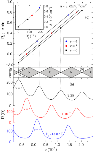
Figure 3: (Color online) (a) Resistance vs. strain traces for the same sample as in Fig. 2 but at a higher density, taken at different fillings for a fixed tilt angle, $\theta=74.5^{\circ}$. (b) Landau level fan diagram as a function of $\epsilon$ for $\nu=6$. (c) Valley polarization ($P_{V}$) as a function of $\epsilon$ at different fillings. The intercepts of the lines with the $y$ axis give $P_{V}$ (or alternatively, $\Delta n$) for the corresponding values of $B_{\parallel}$. Inset shows $\Delta n$ as a function of $B_{\parallel}^{2}$.

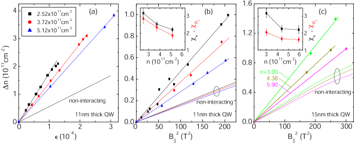
Figure 4: (Color online) (a) Summary of density imbalance as function of $\epsilon$ for three densities for the 11 nm-wide QW. (b) and (c) Summary of density imbalance as function of $B_{\parallel}^{2}$ for three densities for the 11 nm-wide and 15 nm-wide AlAs QWs. Insets show the valley susceptibilities, normalized to their band values, with respect to two variables, $\epsilon$ and $B_{\parallel}^{2}$.

To summarize our results, in Figs. 4(a) and (b) we plot the measured $\Delta n$ vs. $\epsilon$ and vs. $B_{\parallel}^{2}$, respectively, for the 11 nm-wide AlAs QW at three different densities. The data in Fig. 4(a) were obtained from lines such as those shown in Fig. 3 (c), but after subtracting their intercepts with the $\Delta n$ axis. Figure 4(a) data essentially represent $\Delta n$ vs. $\epsilon$ in the absence of $B_{\parallel}$; this can be verified from comparison of the data with measurements reported in Ref. GunawanPRL2006 which were done at $\theta=0$. In Fig. 4(a) we also include a plot of $\Delta n$ vs. $\epsilon$ expected based on the band parameters, i.e., ignoring electron-electron interaction and using the simple relation $\Delta n=\epsilon E_{2}m/2\pi\hbar^{2}$ where $m=\sqrt{m_{l}m_{t}}=0.46$ and $E_{2}$=5.8 eV is the deformation potential for the AlAs X-point conduction band minimum ShayeganPSS2006 . In Fig. 4(a), it is clear that the response of the system to strain is two to three times enhanced compared to what the non-interacting (band) parameters predict, and that the enhancement is stronger at lower densities (larger $r_{s}$). This observation confirms the enhancement of valley susceptibility with respect to strain ($\chi_{\epsilon}$), defined as the rate of change of $\Delta n$ with $\epsilon$, originally reported in Ref. GunawanPRL2006 ; it is similar to the enhancement of the spin susceptibility observed in similar samples and reflects the role of electron-electron interaction ShkolnikovPRL2004 ; GunawanPRL2006 ; GokmenPRB2007 .

Our measured $\Delta n$ caused by $B_{\parallel}$ are plotted in Fig. 4(b) vs. $B_{\parallel}^{2}$ for the same three densities as in Fig. 4(a). Again, for comparison, we also show the results of the calculations based on the non-interacting picture, i.e., using Eq. (4). As can be seen in Eq. (4), there is a slight dependence of $\Delta n$ on $n$ and this is why there are three lines in Fig. 4(b) representing the non-interacting calculations footnote2 . Similar to the strain case of Fig. 4(a), the system’s response to $B_{\parallel}^{2}$ is about two to three times stronger than the non-interacting calculations predict. This is a noteworthy result as it demonstrates that the interacting 2DES responds to two very different stimuli (strain and $B_{\parallel}$) in a very similar fashion. Defining a new quantity, $\chi_{B_{\parallel}}$, as the valley susceptibility with respect to $B_{\parallel}^{2}$, we see from the inset to Fig. 4(b) that $\chi_{\epsilon}$ and $\chi_{B_{\parallel}}$ have very similar magnitudes footnote1 .

In Fig. 4(c) we show the summary of $B_{\parallel}$-induced $\Delta n$ for a second sample, a 2DES confined to a 15 nm-wide AlAs QW. The data overall are quite similar to the 11 nm-wide QW data. The larger well-width of the 15 nm-wide sample predicts a larger $\Delta n$ for this sample (at a given density) because of a larger spread of the wave function in the $z$ direction (see Eq. (2)). The deduced, normalized susceptibilities plotted in Fig. 4(c) inset, however, appear to be slightly smaller than those for the 11 nm-wide sample. It is likely that this is also related to the larger electron layer thickness: Although there have been no systematic and detailed studies of the dependence of $\chi_{\epsilon}$ enhancement on electron layer thickness, it has been reported that the $spin$ susceptibility of a thicker electron system is less enhanced compared to a thinner system with otherwise the same parameters DePaloPRL2005 ; GokmenPRB2007 .

Our results demonstrate that a magnetic field applied parallel to an AlAs 2DES with finite layer thickness can split the energies of the two in-plane valleys. The splitting originates from the coupling of the parallel field to the orbital motion of the electrons. Our measurements of the density imbalance due to strain and parallel magnetic field show similar enhancements of the splitting compared to calculations which are based on non-interacting electrons with band parameters. These enhancements are more pronounced at lower densities (larger $r_{s}$). The results suggest that in an interacting 2DES, the valley splitting is enhanced by interaction, independent of the physical parameter that induces the splitting.

We thank the NSF for support, and R. Winkler for useful discussions. Part of this work was done at the NHMFL, Tallahassee, which is also supported by the NSF. We thank E. Palm, T. Murphy, J. Jaroszynski, S. Hannahs and G. Jones for assistance.

References

- (1) G. Dorda, I. Eisele, and H. Gesch, Phys. Rev. B 17, 1785 (1978).
- (2) T. Ando, A. B. Fowler, and F. Stern, Rev. Mod. Phys. 54, 437 (1982).
- (3) K. Eng, R. N. McFarland, and B. E. Kane, Phys. Rev. Lett. 99, 016801 (2007); and references therein.
- (4) A. K. Geim and K. S. Novoselov, Nature Materials 6, 183 (2007).
- (5) O. Gunawan, E. P. De Poortere, and M. Shayegan, Phys. Rev. B 75, 081304(R) (2007).
- (6) O. Gunawan, T. Gokmen, Y. P. Shkolnikov, E. P. De Poortere, and M. Shayegan, Phys. Rev. Lett. 100, 036602 (2008).
- (7) A. Rycerz, J. Tworzydlo, C. W. J. Beenakker, Nature Physics 3, 172 (2007).
- (8) K. Takashina, A. Fujiwara, S. Horiguchi, Y. Takahashi and Y. Hirayama, Phys. Rev. B 69, 161304(R) (2004).
- (9) A strong perpendicular magnetic field also splits the valley degeneracy. This splitting, which is generally believed to result from electron-electron interaction, leads to ferromagnetic quantum Hall states at odd fillings, some of which have valley Skyrmions as their low-lying excitations. For details, see: Y. P. Shkolnikov, S. Misra, N. C. Bishop, E. P. De Poortere, and M. Shayegan, Phys. Rev. Lett. 95, 066809 (2005).
- (10) F. Stern, W. E. Howard Phys. Rev. 163, 816 (1967).
- (11) F. Stern, Phys. Rev. Lett. 21, 1687 (1968).
- (12) E. Batke and C. W. Tu, Phys. Rev. B 34, 3027 (1986).
- (13) U. Kunze, Phys. Rev. B 35, 9168 (1987).
- (14) E. Tutuc, S. Melinte, E. P. De Poortere, M. Shayegan and R. Winkler, Phys. Rev. B 67, 241309(R) (2003).
- (15) E. P. De Poortere, Y. P. Shkolnikov, E. Tutuc, S. J. Papadakis, M. Shayegan, E. Palm, and T. Murphy, Appl. Phys. Lett. 80, 1583 (2002).
- (16) M. Shayegan, E. P. De Poortere, O. Gunawan, Y. P. Shkolnikov, E. Tutuc, and K. Vakili, Phys. Stat. Sol. (b) 243, 3629 (2006); and references therein.
- (17) O. Gunawan, Y. P. Shkolnikov, K. Vakili, T. Gokmen, E. P. De Poortere, and M. Shayegan, Phys. Rev. Lett. 97, 186404 (2006).
- (18) Y. P. Shkolnikov, K. Vakili, E. P. De Poortere, and M. Shayegan, Phys. Rev. Lett. 92, 246804. (2004).
- (19) T. Gokmen, M. Padmanabhan, E. Tutuc, M. Shayegan, S. De Palo, S. Moroni, and G. Senatore, Phys. Rev. B 76, 233301 (2007)
- (20) As can be seen from Eq. (4), the mass enhancement leads to a decrease in . For example, for the 11 nm-wide sample, the diamagnetic shift and the mass enhancement lead to of cm-2 and cm-2, respectively at cm-2 and T. For the 15 nm-wide sample, these values are cm-2 and cm-2, at cm-2 and T.
- (21) We define as the rate of change of with , and both and in Figs. 4(b) and 4(c) insets are normalized to their band values.
- (22) S. De Palo, M. Botti, S. Moroni, and G. Senatore, Phys. Rev. Lett. 94, 226405 (2005).