In this Supporting information we provide background information on our model of the bacterial flagellar motor. We also derive the analytical solution of our coarse-grained model of the switching dynamics and explain the hybrid stochastic algorithm used for the simulations.

I The model of the bacterial flagellar motor

I.1 Stator-Rotor interaction

The model for the stator-rotor interaction is discussed in the sections The stator-rotor interaction and The rotor switching dynamics of the main text. The model is based on the model of Oster and Blair and coworkers Xing et al. (2006); Kojima and Blair (2001), but extended to include the conformational transitions of the rotor protein complex. Here, we discuss aspects of the model that are not discussed in the main text. But, for completeness, we also give the main equations already presented in the main text.

In our model, each stator-rotor interaction is described by 4 energy surfaces, $U_{s_{j}}^{r}$, with the subscript $s_{j}=0,1$ denoting the conformationals state of stator protein $j$ and the supersript $r=0,1$ denoting the conformational state of the rotor (clockwise or counterclockwise). We assume that the stator proteins are fixed by the peptidoglycan layer and that only the rotor complex moves. The equation-of-motion of the rotor is then given by

$$\gamma_{\rm R}\frac{d\theta_{\rm R}}{dt}=-\sum_{j=1}^{N_{\rm S}}\frac{\partial U^{r}_{s_{j}}(\theta_{j})}{\partial\theta_{\rm R}}+F_{\rm L}+\eta_{\rm R}(t).$$ (1)

Here, $\gamma_{\rm R}$ is the friction coefficient of the rotor; $U^{r}_{s_{j}}(\theta_{j})$ is the free-energy surface shown in Fig. 2 of the main text, where $\theta_{j}=\theta_{\rm R}-\theta_{{\rm S}_{j}}$, with $\theta_{\rm R}$ the rotor rotation angle and $\theta_{{\rm S}_{j}}$ the fixed angle of stator protein $j$; $\eta_{\rm R}(t)$ is a Gaussian white noise term of magnitude $\sqrt{2k_{\rm B}T\gamma_{\rm R}}$; $N_{\rm S}$ is the number of stator proteins. The torque $F_{\rm L}$ denotes the external load. As discussed in Elston and Peskin (2000); Elston et al. (2000); Xing et al. (2006), for the system studied here, the torque-speed curves under conservative load and viscous load are identical. However, as discussed in the main text, the type of load does markedly affect the CW $\leftrightarrow$ CCW switching dynamics.

The transition (or hopping) rate for a stator protein to go from one energy surface to another depends upon the free-energy barrier separating the two surfaces. We make the natural phenomenological assumption that the hopping rate depends exponentially on the free-energy difference, in a manner that obeys detailed balance. Furthermore, following Blair and Oster and coworkers, we assume that the access of the periplasmic protons to the stator-binding sites is triggered by a rotor-stator interaction Kojima and Blair (2001); Xing et al. (2006). This yields the following expression for the hopping rates:

$$k^{r}_{s_{j}\to s_{j}^{\prime}}(\theta_{j})=k_{0}w(\theta_{j})\exp[\Delta U_{ss^{\prime}}(\theta_{j})/2],\,\,\,s,s^{\prime}=0,1.$$ (2)

Here, $k_{0}$ sets the basic time scale, and $\Delta U_{ss^{\prime}}(\theta_{j})=U_{s^{\prime}}(\theta_{j})-U_{s}(\theta_{j})$. The function $w(\theta_{j})$ describes the proton hopping windows (see Fig. 2 of the main text), which reflect the idea that the ion channel through the stator is gated by the motion of the rotor.

The rotor complex is modeled as an MWC model Monod et al. (1965), which means that all the rotor proteins switch conformation in concert. This leads to the following expression for the instantaneous switching rate:

$$k^{r\to r^{\prime}}(\{\theta_{j}\})=\tilde{k}_{0}\exp[\Delta U^{rr^{\prime}}(\{\theta_{j}\})/2],\,\,r,r^{\prime}=0,1,$$ (3)

where $\Delta U^{rr^{\prime}}(\{\theta_{j}\})=\sum_{j=1}^{N_{\rm S}}U_{s_{j}}^{r^{\prime}}(\theta_{j})-U_{s_{j}}^{r}(\theta_{j})$. The average, effective switching rate is given by

$$k_{\rm switch}^{r\to r^{\prime}}=\int d\theta_{\rm R}P(\theta_{\rm R})k^{r\to r^{\prime}}_{s_{j}}(\{\theta_{j}\}),$$ (4)

where $P(\theta_{\rm R})$ is the stationary distribution of the rotor’s position. The instantaneous switching rate $k^{r\to r^{\prime}}_{s_{j}}(\{\theta_{j}\})$ does not depend upon the load. Indeed, in our model, the load does not directly affect the probability that the rotor proteins switch conformation. In this respect, the mechanism that we propose differs fundamentally from that often used to explain the force dependence of processes such as protein unfolding and molecular dissociation Howard (2001); in that mechanism one assumes that the reaction coordinate can described by a single order parameter, and that the force directly couples to that coordinate, changing the relative stability of the two (meta)stable states, as well as the location and stability of the transition state separating them. In our model, the propensity for the rotor to switch depends on interactions with the stator proteins. Consequently, the reaction coordinate for switching depends not only on the coordinate describing the conformational state of the rotor protein complex, but also on the coordinates describing the positions and the conformational of the stator proteins. While the load may change the free-energy landscape in the direction describing the conformational state of the rotor, we assume that the load only couples to the rotation direction of the rotor. The load thus changes the steady-state distribution of the rotor’s position relative to that of the stator proteins, which in turn affects how often during their motor cycle the stator proteins favor one conformational state of the rotor protein complex over the other. In other words, while increasing the load does not change the instantaneous switching rate $k^{r\to r^{\prime}}_{s_{j}}(\{\theta_{j}\})$, it does shift $P(\theta_{\rm R})$ to positions $\theta_{\rm R}$ where $k^{r\to r^{\prime}}_{s_{j}}(\{\theta_{j}\})$ is large. This is the principal mechanism that, according to our model, makes the effective switching rate $k_{\rm switch}^{r\to r^{\prime}}$ sensitive to load and speed.
The load In the experiments of Korobkova et al. the motion of the flagellum is visualized via a latex bead connected to the flagellar filament Korobkova et al. (2004, 2006). The bead exerts a force on the rotor protein, which, effectively, tilts the energy surfaces shown in Fig. 2 of the main text. When a) the connection between the load and the motor is soft, b) the dynamics of the motor is much faster than that of the load, and c) chemical transitions lead on average to a fixed translation distance of the rotor, as in the current model, then the torque-speed curves under conservative load and viscous load are identical Elston and Peskin (2000); Elston et al. (2000); Xing et al. (2006). However, as discussed in the main text, the type of load does markedly affect the CW $\leftrightarrow$ CCW switching dynamics.

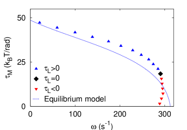
Figure 1: The torque-speed relation (symbols)as predicted by the model used here, which is based on the model of Oster et al. Xing et al. (2006). The blue symbols correspond to the regime in which the load pulls the motor in the backward direction; the red symbols correspond to the regime in which the load pulls the motor in the forward direction, which is the scenario right after a switching event. The line shows that, to a good approximation, the speed $\omega$ as a function of the motor torque $\tau_{\rm M}$, is given by the speed as a function of the conservative load $\tau_{\rm L}$, according to $\omega=(k_{\rm hop}^{+}-k_{\rm hop}^{-})\pi/26$, where the hopping rates in the forward (+) and backward (-) are given by $k_{\rm hop}^{\pm}=\int_{0}^{2\pi/26}d\theta P_{\rm S}(\theta)k^{\pm}(\theta)$, and the stationary distribution $P_{\rm S}(\theta)$ is approximated by the equilibrium distribution $P_{\rm eq}(\theta)\propto\exp(-\beta\left[U_{s}(\theta)+\tau_{\rm L}\theta\right])$ (See Ref. Van Albada (2008)). The parameters used in the simulations are shown in Table 1.

The stator proteins Resurrection experiments suggest that in vivo the number of stator proteins is around $8-12$ Ryu et al. (2000); Reid et al. (2006). At high load, the stator proteins act cooperatively, and the motor speed increases with the number of stator proteins Ryu et al. (2000); the model of Oster and coworkers describes this observation Xing et al. (2006). Recent experiments by Yuan Berg show that near zero external load, the speed is independent of the number of stator proteins Yuan and Berg (2008). The model of Oster and coworkers can reproduce this behavior if the stator proteins are connected to the rigid framework of the cell wall via very soft springs. However, to generate a speed that is independent of the number of stator proteins, the springs have to be made so soft that they stretch a distance of order 10 nm, which, as Yuan and Berg point out, seems unlikely Yuan and Berg (2008). We therefore focus here on a motor that has only one stator protein that is rigidly connected to the cell membrane. This motor has a lower maximum torque than a “wild-type”motor with 8-12 stator proteins, but this is not critical, since we take a rather small bead (see table 1); in essence, to a good approximation, all the torques in our model could be scaled by the number of stator proteins. More importantly, our model correctly predicts the maximum speed of about 300 Hz, as recently observed by Yuan and Berg Yuan and Berg (2008), and its torque-speed relation exhibits the distinc knee at a speed of about 250 Hz (see Fig. 1). This model thus captures the effect of the dynamical interplay between the torque and the speed, and on the other hand the switching dynamics. The maximum speed is particularly important, since that, together with the total change in the winding angle of the flagellar filament upon a motor reversal, directly affects the characteristic switching time. In future work, we will investigate the effect of the number of stator proteins on the switching dynamics.

The parameters of the rotor-stator model, which were mostly taken from Xing et al. (2006), are summarized in table 1.

Parameter	Value	Description
$d$	$2\pi~{}{\rm rad}/26$	Potential periodicity
pmf	152 mV	Proton-motive force
$\Delta G$	$11.8~{}k_{\rm B}T$	$\Delta G=2e\times{\rm pmf}$
$k_{0}$	$3.5~{}10^{4}~{}{\rm s}^{-1}$	Hopping prefactor
$d_{1}$	$0.05~{}d$	Position potential maximum
$d_{2}$	$0.1~{}d$	Position start power stroke
$d_{3}$	$0.9~{}d$	Center of hopping window
$d_{4}$	$0.2~{}d$	Width of hopping window
$h_{1}$	$25~{}k_{\rm B}T$	Height potential maximum
$h_{2}$	$10~{}k_{\rm B}T$	Height start power stroke
$F_{\rm M}=-h_{2}/(d-d_{2})$	$46~{}k_{\rm B}T~{}{\rm rad}^{-1}$	Force motor during power stroke
$\gamma_{\rm M}$	$1.7~{}10^{-3}~{}{\rm s}~{}{\rm rad}^{-2}$	Friction coefficient motor
$\tilde{k}_{0}$	$0.3~{}{\rm s}^{-1}$	Switching prefactor
$\gamma_{\rm L}$	$0.51k_{\rm B}T~{}{\rm s}~{}{\rm rad}^{-2}$	Friction coefficient load

Table 1: Parameters for the rotor-stator model as used in the simulations (see also Xing et al. (2006)).

I.2 Elasticity of the flagellar filament

We assume that the free energy of a flagellar filament in a given polymorphic state $m$ is quadratic in the curvature $\kappa$ and torsion $\tau$:

$$U^{\rm F}_{m}(\tau,\kappa)/L=\frac{1}{2}EI(\kappa-\kappa_{m})^{2}+\frac{1}{2}\mu J(\tau-\tau_{m})^{2},$$ (5)

where $L$ is the contour length, $E$ and $\mu$ are the Young’s and shear moduli, $I$ and $J$ are cross-sectional moments, and $\kappa_{m}$ and $\tau_{m}$ are, respectively, the spontaneous curvature and torsion of the filament in state $m$. The curvature and torsion are functions of the height $z$ and the winding angle $\theta$:

$$\kappa(\theta,z) = \frac{\theta\sqrt{L^{2}-z^{2}}}{L^{2}},$$ (6)

$$\tau(\theta,z) = \frac{\theta z}{L^{2}}.$$ (7)

We assume that at each instant the length of the filament has relaxed to its steady state value $z_{\rm eq}(\theta)$, obtained as a solution of the equation $\frac{\partial U(\tau(\theta,z),\kappa(\theta,z))}{\partial z}=0$. This allows us to elimate $z$ and express the “torsional” energy as a function of the winding angle $\theta$:

$$U^{\rm T}_{m}(\theta)=U^{\rm F}_{m}(\tau(\theta,z_{\rm eq}(\theta)),\kappa(\theta,z_{\rm eq}(\theta))),$$ (8)

The function $U^{\rm F}_{m}(\theta)$ is, in general, a complicated fonction of $\theta$; nevertheless in the limit of equal bending and twisting stifnesses ($EI=\mu J$) Darnton and Berg (2007 Mar 15) the torsion potential corresponds to a linear elastic potential

$$U^{\rm F}_{m}(\theta)=\frac{1}{2}k_{\theta}(\theta-\theta_{m})^{2},$$ (9)

where $k_{\theta}=\frac{EI}{L}$ and $\theta_{m}=\frac{\sqrt{\kappa_{m}^{2}+\tau_{m}^{2}}}{L}$. The eperimental data of Darnton and Berg Darnton and Berg (2007 Mar 15) confirm that the approximation $EI\simeq\mu J$ is valid and therefore, locally, the potential energy guiding the dynamics of the twisting angle $\theta$ has a simple linear elasticity form with elastic constant $k_{m}\simeq 100$ pN nm/${\rm rad}^{2}$ (obtained from $EI=\mu J=3.5$ pN ${\rm\mu}m^{2}$ and $L=7.6,19.6$ ${\rm\mu}$m as in Darnton and Berg (2007 Mar 15)). As described in the main text, we assume that the potentiall wells are equally spaced, are of the same depth and have the same curvature. Clearly, these assumptions could be relaxed by allowing, e.g., the normal state to be more stable and to have a higher stiffness.

Motivated by the observations of Darnton and Berg Darnton and Berg (2007 Mar 15), we assume that the transition from one polymorphic state to another is an activated process, with a rate constant given by

$$k_{m\to m^{\prime}}(\theta)=\breve{k}_{0}\exp[(U^{\rm F}_{m}(\theta)-U^{\rm F}_{m^{\prime}}(\theta))/2].$$ (10)

The equation-of-motion for the bead is given by

$$\gamma_{\rm L}\frac{d\theta_{\rm L}}{dt}=-k_{\theta}(\theta_{\rm L}-\theta_{\rm R}-\theta_{m})+\eta_{\rm L}(t).$$ (11)

Here, $\gamma_{\rm L}$ is the friction coefficient of the bead, and $\eta_{\rm L}$ is a Gaussian white noise term of magnitude $\sqrt{2k_{\rm B}T\gamma_{\rm L}}$.

The parameters of the model are given in table 2.

Parameter	Value	Description
$\theta_{m}-\theta_{m-1}$	$150d$	Spacing of wells
$k_{\theta}$	$1k_{\rm B}T/{\rm rad}^{2}$	Stiffness
$N$	10	Number of wells.
$\breve{k}_{0}$	$10^{-6}{\rm s}^{-1}$	Jumping prefactor

Table 2: Parameters describing the flagellar filament.

II Coarse grained model of the switching dynamics

We model the switching dynamics as a memoryless two-state system with switching-time distributions $\psi_{+}(t)$ switching from CW to CCW and $\psi_{-}(t)$ for switching from CCW to CW:

$$\mathrm{CW}\underset{\psi_{-}(t)}{\overset{\psi_{+}(t)}{\rightleftarrows}}\mathrm{CCW}$$ (12)

Lack of memory means in this context that the probability to switch from one state depends only on the time since the transition to that state – the system forgets everything before the last transition.

The switching-time distribution is related to the switching rate or switching propensity (the switching probability per unit amount of time) $k_{\alpha}(t)$ as

$$\psi_{\alpha}(t)=k_{\alpha}(t)\text{e}^{-\int_{0}^{t}k_{\alpha}(t^{\prime})dt^{\prime}}.$$ (13)

One important characteristic of the stochastic trajectory of the system is the correlation function $C(t)$ of the characteristic function $\chi(t)$:

$$C(t)=\langle{\chi(t)\chi(0)}\rangle-\langle{\chi}\rangle^{2}.$$ (14)

We take $\chi(t)=1$ if the system is in the CW state and $\chi(t)=0$ otherwise. From the ensemble of all possible trajectories only the ones that are in the CW state both at time zero and at time $t$ contribute to the correlation function at time $t$. Therefore, one can write the correlation function as

$$C(t)=\left[P({\rm CW},t;{\rm CW},0)-P({\rm CW},\infty;{\rm CW},0)\right]P({\rm CW},\infty;{\rm CW},0),$$ (15)

where $P({\rm CW},t;{\rm CW},0)$ is the probability that a trajectory is in the CW state at time $t$ given that it starts in that state at time zero. Using a well established result in the theory of (alternating) two-state, memoryless renewal processes (see Cox (1961), Chapter 7) one can express this quantity in the Laplace domain as:

$$\tilde{P}(z)=\frac{1}{z}\left(1-\frac{G(z)}{zt_{\rm CW}}\right).$$ (16)

Here, $\tilde{P}(z)$ is the Laplace transform of $P({\rm CW},t;{\rm CW},0)$,

$$\tilde{P}(z)=\int_{0}^{\infty}P({\rm CW},t;{\rm CW},0)\text{e}^{-zt}dt,$$ (17)

$G(z)$ is a function that depends on the Laplace transformed switching-time distributions,

$$G(z)=\frac{(1-\tilde{\psi}_{+}(z))(1-\tilde{\psi}_{-}(z))}{(1-\tilde{\psi}_{-}(z)\tilde{\psi}_{+}(z))},$$ (18)

and $t_{\rm CW}$ is the average residence time in the CW state. The probability to be in the CW state is given by the average residence times as

$$P({\rm CW},\infty;{\rm CW},0)=\frac{t_{\rm CW}}{t_{\rm CW}+t_{\rm CCW}}.$$ (19)

Also, using the properties of the Laplace transform one has

$$\tilde{C}(z)=\frac{t_{\rm CW}}{t_{\rm CW}+t_{\rm CCW}}\left[\tilde{P}(z)-\frac{t_{\rm CW}}{z(t_{\rm CW}+t_{\rm CCW})}\right].$$ (20)

Once we have the correlation function, we can compute the power spectrum using the formula

$$S(\omega)=2\int_{0}^{\infty}C(t)\cos{\omega t}=\tilde{C}(\text{i}\omega)+\tilde{C}(-\text{i}\omega),$$ (21)

such that

$$S(\omega)=\frac{1}{\omega^{2}(t_{\rm CW}+t_{\rm CCW})}\left[G(\text{i}\omega)+G(-\text{i}\omega)\right].$$ (22)

A       B

Figure 2: A) A piecewise linear model of the switching-propensity function $k(t)$. B) Computed power spectrum $S(\omega)$.

In general, an analytical formula for the power spectrum $S(\omega)$ cannot be obtained for any arbitrary switching-propensity function $k_{\alpha}(t)$. Nevertheless, one can obtain an analytical formula for the power spectrum if the switching-propenstiy function is piecewise linear, as in Fig. 2A. Fig. 2B shows the power spectrum for a symmetric system, with switching-propensity functions in the forward and backward directions as shown in Fig. 2A. It is seen that this simple, non-Markovian two-state model can capture the main features of the power spectrum as measured by Korobkova et al.Korobkova et al. (2006).

III Hybrid stochastic algorithm

The equations-of-motion for the rotor and the flagellum, Eqs. 1 and 7 of the main text, respectively, and Eqs. 1 and 11 above, are propagated via a Heun scheme Greiner et al. (1988).

The algorithm to determine when the next hopping, switching, or polymorphic transition will occur is essentially a kinetic Monte Carlo algorithm Bortz et al. (1975). It is based on the observation that the survival probability $S(t)$, i.e. the probability that no hopping, switching or polymorphic transition has happened after a time $t$ after the last event, is given by

$$S(t)=\exp\left(-a(t)\right),$$ (23)

where $a(t)$ is the cumulative total propensity function:

$$a(t)=\int_{0}^{t}dt^{\prime}k_{\rm T}(t^{\prime}),$$ (24)

with $k_{\rm T}(t)$ being the total propensity function as given by

$$k_{\rm T}(t)=\sum_{j=1}^{N_{\rm S}}k^{r}_{s_{j}\to s_{j}^{\prime}}(\theta_{j}(t))+k^{r\to r^{\prime}}(\{\theta_{j}(t)\})+k_{m\to m^{\prime}}(\theta_{\rm L}(t)-\theta_{\rm R}(t)-\theta_{m})).$$ (25)

In practice, right after a hopping, switching or polymorphic transition, a random number, $\xi$, between zero and one is drawn. The equations-of-motion of the rotor and the flagellum are then integrated together with the equation that describes the temporal evolution of $a(t)$:

$$\frac{da(t)}{dt}=k_{\rm T}(t).$$ (26)

Integrating Eq. 26 since the last event leads to an estimate for $a(t)=\int_{0}^{t}dt^{\prime}k_{\rm T}(t^{\prime})$. The next event then occurs after a time $t$ since the last event when

$$a(t)>\log(1/\xi).$$ (27)

The event type $\alpha$, where $\alpha$ is either a hopping, switching, or polymorphic transition, is subsequently chosen with a probability $p_{\alpha}$ as given by

$$p_{\alpha}(t)=k_{\alpha}(t)/k_{\rm T}(t).$$ (28)

References

- Xing et al. (2006) J. Xing, F. Bai, R. Berry, and G. Oster, Proc Natl Acad Sci U S A 103, 1260 (2006), ISSN 0027-8424 (Print).
- Kojima and Blair (2001) S. Kojima and D. F. Blair, Biochemistry 40, 13041 (2001).
- Elston and Peskin (2000) T. C. Elston and C. S. Peskin, Siam J. App. Math 60, 842 (2000).
- Elston et al. (2000) T. C. Elston, D. You, and C. S. Peskin, Siam J. App. Math 61, 776 (2000).
- Monod et al. (1965) J. Monod, J. Wyman, and J.-P. Changeux, J. Mol. Biol. 12, 88 (1965).
- Howard (2001) J. Howard, Mechanics of Motor Proteins and the Cytoskeleton (Sinauer Associates, Inc., 2001).
- Korobkova et al. (2004) E. A. Korobkova, T. Emonet, J. M. G. Vilar, T. S. Shimizu, and P. Cluzel, Nature 428, 574 (2004).
- Korobkova et al. (2006) E. A. Korobkova, T. Emonet, H. Park, and P. Cluzel, Phys. Rev. Lett. 96, 058105 (2006).
- Van Albada (2008) S. B. Van Albada, Ph.D. thesis, Vrije Universiteit Amsterdam (2008).
- Ryu et al. (2000) W. S. Ryu, R. M. Berry, and H. C. Berg, Nature 403, 444 (2000).
- Reid et al. (2006) S. W. Reid, M. C. Leake, J. H. Chandler, C.-Y. Lo, J. P. Armitage, and R. M. Berry, Proc. Natl. Acad. Sci. USA 101, 8066 (2006).
- Yuan and Berg (2008) J. Yuan and H. C. Berg, Proc. Natl. Acad. Sci. USA 105, 1182 (2008).
- Darnton and Berg (2007 Mar 15) N. C. Darnton and H. C. Berg, Biophys J 92, 2230 (2007 Mar 15), ISSN 0006-3495 (Print).
- Cox (1961) D. R. Cox, Renewal Theory (Chapman and Halt, London, 1961).
- Greiner et al. (1988) A. Greiner, S. W, and H. J, jsp 51, 95 (1988).
- Bortz et al. (1975) A. B. Bortz, M. H. Kalos, and J. L. Lebowitz, J. Comp. Phys. 17, 10 (1975).