Dynamic heterogeneities in critical coarsening: Exact results for correlation and response fluctuations in finite-sized spherical models

Abstract

We study dynamic heterogeneities in the out-of-equilibrium coarsening dynamics of the spherical ferromagnet after a quench from infinite temperature to its critical point. A standard way of probing such heterogeneities is by monitoring the fluctuations of correlation and susceptibility, coarse-grained over mesoscopic regions. We discuss how to define such fluctuating coarse-grained correlations and susceptibilities in models where no quenched disorder is present. Our focus for the spherical model is on coarse-graining over the whole volume of $N$ spins, which requires accounting for ${{\mathcal{O}}}(N^{-1/2})$ non-Gaussian fluctuations of the spin variables. The latter are treated as a perturbation about the leading order Gaussian statistics. We obtain exact results for these quantities, which enable us to characterize the joint distribution of correlation and susceptibility fluctuations. We find that this distribution is qualitatively different, even for equilibrium above criticality, from the spin-glass scenario where correlation and susceptibility fluctuations are linked in a manner akin to the fluctuation-dissipation relation between the average correlation and susceptibility. Our results show that coarsening at criticality is clearly heterogeneous above the upper critical dimension and suggest that, as in other glassy systems, there is a well-defined timescale on which fluctuations across thermal histories are largest. Surprisingly, however, neither this timescale nor the amplitude of the heterogeneities increase with the age of the system, as would be expected from the growing correlation length. Below the upper critical dimension, the strength of correlation and susceptibility fluctuations varies on a timescale proportional to the age of the system; the corresponding amplitude also grows with age, but does not scale with the correlation volume as might have been expected naively.

1 Introduction

Dynamic heterogeneities, where different local regions of a system evolve on different timescales, arise in many non-equilibrium situations. Their existence in supercooled liquids and other glassy systems has been probed experimentally using techniques including light scattering and confocal microscopy [1, 2, 3, 4, 5, 6] and this has been complemented by results from simulation and theory [7, 8, 9, 10, 11, 12, 13, 14, 15].

In systems with quenched disorder such as spin glasses, the disorder itself provides an obvious source of heterogeneous dynamics: spins compelled to assume particular local configurations by the disorder decorrelate slowly, while less constrained ones can lose memory of their configuration at some initial time very quickly. In the aging dynamics of such systems after a quench to low temperature, it has been argued that an invariance of the global dynamics under reparametrization of time also dominates the fluctuations of the local dynamics, with different regions of the system effectively having different ages [16, 17, 18, 19]. In order to study such behaviour it is natural to consider two-time correlation functions and susceptibilities. For a lattice system with $N$ sites labelled by $i$ and spins (or more generally local order parameters) $S_{i}$ these functions are, after spatial coarse-graining over the entire finite-sized system,

$$\hat{C}(t,t_{\rm w}) = \frac{1}{N}\sum_{i}\hat{C}_{ii}(t,t_{\rm w}),\quad\hat{C}_{ii}(t,t_{\rm w})=S_{i}(t)S_{i}(t_{\rm w})$$ (1.1)

$$\hat{\chi}(t,t_{\rm w}) = \frac{1}{N}\sum_{i}\hat{\chi}_{ii}(t,t_{\rm w}),\quad\hat{\chi}_{ii}(t,t_{\rm w})=\frac{\partial S_{i}(t)}{\partial h_{i}(t_{\rm w})}\ .$$ (1.2)

Here $h_{i}$ is the field conjugate to $S_{i}$ and is assumed to have been switched on at the waiting time $t_{\rm w}$ (measured from the time of preparation of the system, e.g. by quenching), with the response measured at the later time $t$. We have used hats to emphasize that the correlator and susceptibility defined above fluctuate across thermal histories (including variability in initial conditions); we return below to what this implies for measuring $\hat{\chi}$. Averaging over the thermal fluctuations gives the conventional correlation and susceptibility, $C=\langle\hat{C}\rangle$ and $\chi=\langle\hat{\chi}\rangle$. In aging systems these are related by an out-of-equilibrium fluctuation-dissipation (FD) relation [20]

$$-\partial_{t_{\rm w}}\chi(t,t_{\rm w})\equiv R(t,t_{\rm w})=\frac{X(t,t_{\rm w})}{T}\partial_{t_{\rm w}}C(t,t_{\rm w})$$ (1.3)

where $R(t,t_{\rm w})$ is the impulse response function, linked to the susceptibility by

$$\chi(t,t_{\rm w})=\int_{t_{\rm w}}^{t}dt^{\prime}\,R(t,t^{\prime})$$ (1.4)

and $X(t,t_{\rm w})$ is the fluctuation-dissipation ratio (FDR). The FDR can be read off from the negative slope of a parametric FD plot showing $T\chi$ versus $C$, at fixed $t$ and with $t_{\rm w}$ varying along the curve. In equilibrium, the FD theorem (see e.g. [21]) implies that the FD plot is a straight line with slope $-1$, corresponding to $X=1$. Out of equilibrium, the prediction from local time reparametrization invariance [16, 17, 18, 19] is that the contour lines of the joint probability distribution of the fluctuating quantities $\hat{C}$ and $T\hat{\chi}$, at fixed $t_{\rm w}$ and $t$, follow the local slope of the FD plot constructed from the average quantities.

An obvious question to ask is whether the fluctuations of correlation and response obey similar constraints in systems without quenched disorder, where dynamic heterogeneities are “self-generated”. There is some evidence for an affirmative answer from simulations of kinetically constrained models of (structural) glasses [22]. Our interest here is in simpler models displaying aging, where we can hope to make progress by analytical calculation, namely coarsening systems [23, 24]. It has been argued that in these full time-reparametrization invariance no longer holds, with only time rescaling remaining as a symmetry in the long-time aging dynamics [25]. This means that there is no obvious reason a priori for the presence of any constraint linking local correlation and response fluctuations to the average FD relation, and our main aim will be to investigate what effects this has on the distributions of the fluctuating quantities.

Coarsening systems are magnetic systems – or their analogues in gas-liquid phase separation, demixing of binary liquids etc – quenched from the high-temperature phase to or below their critical temperature, $T_{\rm c}$, (see e.g. [26, 27] and the review [28]). During the phase ordering (below $T_{\rm c}$) or the critical relaxation (at $T_{\rm c}$), aging occurs due to the growth of a length scale (domain size or correlation length respectively) [29], and in an infinitely large system equilibrium is never reached. At any time there are spins at the interfaces that behave quite differently from the ones inside a domain, so that the origin of dynamic heterogeneities and the associated length scale have a clear physical interpretation. As before one can then consider the resulting fluctuations around average FD plots. For critical coarsening the analysis has to be modified slightly: here the FD plots can in fact hide the interesting aging behaviour of the FDR $X$ [26, 27, 30, 31, 32, 33, 34]. The latter typically is a smooth function of $t_{\rm w}/t$ [26], so that also the fluctuation effects have to be analysed in terms of the same scaling variable.

In this paper we study the fluctuations in the Langevin dynamics of finite-size spherical ferromagnets [35, 36] after a quench from equilibrium at infinite temperature to some low temperature $T$. We will focus mainly on quenches to the critical temperature, but comment also on the behaviour in the equilibrium region above. Our calculation is based on a leading order expansion in $1/N$ of the non-Gaussian fluctuations of the spins, so that we are effectively considering systems of finite but large size $N$. The nature of the expansion prevents us from accessing the phase ordering below $T_{\rm c}$, where as soon as domains are formed the non-Gaussian fluctuations become dominant rather than a small perturbation about the leading order statistics, which are Gaussian in the spherical model. Our results therefore complement those of Ref. [25], where for the case of zero temperature and $N\to\infty$ the fluctuations of correlations were analysed, for coarse-graining volumes ranging from a single site to much larger than the correlation length. The overall scaling of correlation fluctuations in coarsening below $T_{\rm c}$ is well understood and has a clear interpretation in terms of the growing domain size [23]. Our study fills an important gap in allowing us to look at coarsening at criticality, where the connection between dynamical heterogeneities and a growing correlation length is much less clear.

We will first describe, in Sec. 2, how we characterize the fluctuations of coarse-grained correlation and susceptibilities. A discussion is then given of possible alternative definitions of these fluctuating quantities. Some of these can be ruled out as less useful because they give different scalings with system size for the variance of correlations and susceptibilities.

Our analysis proper starts in Sec. 3 with the derivation of the correlation and susceptibility variances and the covariance. We will give general, exact expressions for these quantities in terms of three-time kernels, $D$ and $D^{\chi}$, which will constitute the basis for all our further analysis. Our interest will be in the out-of-equilibrium dynamics of the system after a quench from an initial state of equilibrium at high temperature to its critical temperature. Before considering non-equilibrium, though, we will analyse briefly the situation of a quench to above criticality, (in Sec. 4), where the equilibration process is fast and a genuine equilibrium dynamics takes place. We will first derive the general equilibrium expressions of the relevant quantities and later specilize to the case of high temperature. Even here, the results are new as far we know. In Sec. 5 we will turn to the more interesting case of quenches to criticality. In the regime of small time differences the critical dynamics displayed by the system is stationary and one can look at the equilibrium situation. For larger time differences the aymptotic dynamics in $d>4$ is essentially given by the equilibrium one modulated by relatively weak aging corrections, whereas for $d<4$ one needs to look directly at the non-equilibrium situation. The latter is discussed in Sec. 6. We summarize and look forward to avenues for future research in Sec. 7.

2 Definition of fluctuating correlation and susceptibility

In this section we describe first how we will characterize the fluctuations of the correlator and susceptibility defined in Eqs. (1.1,1.2). We then discuss, and largely rule out, alternative ways of defining fluctuating correlation and response functions that are coarse-grained across an entire finite system.

To the leading order in $1/N$, i.e. inverse system size, that we keep, the joint distribution of the fluctuating correlation and susceptibility is Gaussian and therefore fully characterized by its second moments. Specifically, denoting the fluctuations $\delta C=\hat{C}-C$ and $\delta\chi=\hat{\chi}-\chi$, we will study the behaviour of the variances

$$V_{C}(t,t_{\rm w}) = N\left\langle[\delta C(t,t_{\rm w})]^{2}\right\rangle$$ (2.1)

$$V_{\chi}(t,t_{\rm w}) = NT^{2}\left\langle[\delta\chi(t,t_{\rm w})]^{2}\right\rangle$$ (2.2)

and of the covariance

$$V_{C\chi}(t,t_{\rm w})=NT\left\langle\delta C(t,t_{\rm w})\delta\chi(t,t_{\rm w})\right\rangle$$ (2.3)

Factors of $N$ have been included here to make all three quantities of order unity. Also, as suggested by the equilibrium FD theorem, we have scaled the susceptibility fluctuation $\delta\chi$ by a factor $T$ to obtain a quantity with the same dimension as $\delta C$.

Writing out the variance of the fluctuations of the correlation explicitly as

$$V_{C}(t,t_{\rm w})=\frac{1}{N}\sum_{i,j}\left[\langle\hat{C}_{ii}(t,t_{\rm w})\hat{C}_{jj}(t,t_{\rm w})\rangle-\langle\hat{C}_{ii}(t,t_{\rm w})\rangle\langle\hat{C}_{jj}(t,t_{\rm w})\rangle\right]$$ (2.4)

one sees that this is none other than the by now standard four-point correlation function used to characterize heterogeneous dynamics, often denoted $C_{4}$ or $\chi_{4}$ [11]. For coarsening below $T_{\rm c}$ in spatial dimension $d$, the amplitude of this quantity scales with $\xi^{d}(t_{\rm w})\sim t_{\rm w}^{d/2}$ [23], where $\xi(t_{\rm w})\sim t_{\rm w}^{1/2}$ is the growing domain size. At criticality, $\xi(t_{\rm w})$ – now the lengthscale of regions across which equilibrium correlations are established – will still grow with the same exponent but it is less obvious how it enters $V_{C}$ and the corresponding susceptibility fluctuations. Our explicit results will shed light on this question.

There are other fluctuating correlation and response functions we could have considered. Firstly, instead of coarse-graining over the entire finite-sized system as in (1.1) and (1.2), we could have coarse-grained over regions of finite size (and then gathered statistics also across all possible centre points of such regions). However, for the spherical ferromagnet such a locally coarse-grained susceptibility has negligible fluctuations compared to those of the correlation, as demonstrated (in the context of the leading order Gaussian spin statistics) in [25]. This is why we focus on global coarse-graining, for which non-Gaussian effects make also the response fluctuations non-trivial.

Secondly, our $\hat{\chi}$ from (1.2) requires that we measure separately, for a given noise history, all local susceptibilities $\hat{\chi}_{ii}$. For Langevin dynamics as studied in this paper this does not present a problem since the differentiation w.r.t. the local field $h_{i}$ can be carried out directly, and an explicit equation of motion for $\chi_{ii}$ be written down, in the spirit of a slave estimator (see e.g. [37]). However, already for Markov dynamics simulated via a Monte Carlo scheme it becomes necessary in principle to rerun the dynamics $N$ times, each time switching on one of the local fields, unless specially crafted “field-free” methods are used [38, 39, 40]. It is tempting to avoid this difficulty by using a standard trick for obtaining local responses [41]: one could consider the observable $A=\sum_{i}\epsilon_{i}S_{i}$, with the $\epsilon_{i}$ quenched zero mean random variables. The response of $A$ to its conjugate field, scaled by $1/N$ to give a result of order unity, is then

$$\hat{\chi}_{\epsilon}=\frac{1}{N}\sum_{ij}\epsilon_{i}\epsilon_{j}\hat{\chi}_{ij}.$$ (2.5)

It can be measured with a single rerun of the history (although of course even this is likely to be impossible in a real rather than a numerical experiment). The above procedure, employed in [16, 18], should reduce to the definition (1.2) if the random field amplitudes $\epsilon_{i}$ are drawn without spatial correlation so that, on averaging over their distribution as indicated by the overbar, $\overline{\epsilon_{i}\epsilon_{j}}=\delta_{ij}$. One has to bear in mind, however, that the randomness in the $\epsilon_{i}$ may induce additional fluctuations in $\hat{\chi}_{\epsilon}$ which are not present in $\hat{\chi}$. This does not appear to have been the case for the systems studied in [16, 18], presumably due to the presence there of quenched disorder.

In our case, on the other hand, the variance of $\hat{\chi}_{\epsilon}$ would be genuinely larger than that of $\hat{\chi}$. This can be seen by considering

$$N\langle(\delta\chi_{\epsilon})^{2}\rangle=\frac{1}{N}\sum_{ijkl}\epsilon_{i}\epsilon_{j}\epsilon_{k}\epsilon_{l}\left\langle\delta\chi_{ij}\delta\chi_{kl}\right\rangle=\sum_{j^{\prime}k^{\prime}l^{\prime}}\left(\frac{1}{N}\sum_{i}\epsilon_{i}\epsilon_{i+j^{\prime}}\epsilon_{i+k^{\prime}}\epsilon_{i+l^{\prime}}\right)\left\langle\delta\chi_{0j^{\prime}}\delta\chi_{k^{\prime}l^{\prime}}\right\rangle$$ (2.6)

where we have used that after thermal averaging the response statistics in a system without quenched disorder are translationally invariant. As the statistics of the $\epsilon$ are defined to be likewise translationally invariant, the normalized sum over $i$ can be replaced to leading order by a disorder average, giving

$$N\langle(\delta\chi_{\epsilon})^{2}\rangle=\sum_{j^{\prime}k^{\prime}l^{\prime}}\overline{\epsilon_{0}\epsilon_{j^{\prime}}\epsilon_{k^{\prime}}\epsilon_{l^{\prime}}}\left\langle\delta\chi_{0j^{\prime}}\delta\chi_{k^{\prime}l^{\prime}}\right\rangle=\frac{1}{N}\sum_{ijkl}\overline{\epsilon_{i}\epsilon_{j}\epsilon_{k}\epsilon_{l}}\left\langle\delta\chi_{ij}\delta\chi_{kl}\right\rangle$$ (2.7)

The fourth-order disorder average gives

$$\overline{\epsilon_{i}\epsilon_{j}\epsilon_{k}\epsilon_{l}}=\overline{\epsilon_{i}\epsilon_{j}}\ \overline{\epsilon_{k}\epsilon_{l}}+\overline{\epsilon_{i}\epsilon_{k}}\ \overline{\epsilon_{j}\epsilon_{l}}+\overline{\epsilon_{i}\epsilon_{l}}\ \overline{\epsilon_{j}\epsilon_{k}}$$ (2.8)

This is exactly true if the $\epsilon$ are taken as Gaussian variables; for e.g. binary variables $\epsilon_{i}=\pm 1$ one gets an extra term $-2\delta_{ij}\delta_{ik}\delta_{il}$ but this makes a subleading contribution in $1/N$. Overall one has

$$N\langle(\delta\chi_{\epsilon})^{2}\rangle=\frac{1}{N}\sum_{ij}\left[\langle\delta\chi_{ii}\delta\chi_{jj}\rangle+2\langle(\delta\chi_{ij})^{2}\rangle\right]$$ (2.9)

Comparing with (1.2) one sees that this is indeed larger than $N\langle(\delta\chi)^{2}\rangle$, by the second term in the square brackets of (2.9). As an aside, we note that (2.7) can be written as $\langle(\delta\chi_{\epsilon})^{2}\rangle=\overline{\langle(\delta\chi_{\epsilon})^{2}\rangle}$, i.e. the variance of $\delta\chi_{\epsilon}$ is self-averaging with respect to the sampling of the field amplitudes $\epsilon$. The same argument can be applied to all other moments of $\hat{\chi}_{\epsilon}$, so that the entire distribution $P(\hat{\chi}_{\epsilon})$ is self-averaging. The increased variance of $\hat{\chi}_{\epsilon}$ is therefore present for any given sample of the $\epsilon$. It does not arise, as one might alternatively have suspected, by $\hat{\chi}_{\epsilon}$ for each sample $\epsilon$ having a distribution similar to that of $\hat{\chi}$ but with a shifted mean that fluctuates with $\epsilon$.

The difference between $\hat{\chi}_{\epsilon}$ and $\hat{\chi}$ can be avoided by averaging over a sufficiently large number of different configurations of the $\epsilon_{i}$. (This of course means that an appropriate number of reruns of each thermal history are required, defeating to a certain extent the object of working with the random field amplitudes $\epsilon_{i}$.) One thus effectively “preaverages” over $\epsilon$; allowing for a general covariance $\overline{\epsilon_{i}\epsilon_{j}}\equiv\epsilon_{ij}$ this gives

$$\hat{\chi}=\frac{1}{N}\sum_{ij}\epsilon_{ij}\hat{\chi}_{ij}$$ (2.10)

It is this form that we will use in the calculations below, with $\epsilon_{ij}$ short-ranged (so that $\sum_{j}\epsilon_{ij}=\mathcal{O}(1)$). The extreme long-range case $\epsilon_{ij}=1$ corresponds to spatially uniform, non-disordered, fields $\epsilon_{i}=1$ and so would be easiest to measure, with only a single rerun of the thermal history. The observable $A$ then simplifies to $A=\sum_{i}S_{i}=Nm$ so that $\hat{\chi}$ becomes the magnetization susceptibility $\hat{\chi}_{m}$. Its (scaled) variance can be written as

$$N\langle(\delta\chi_{m})^{2}\rangle=\frac{1}{N}\sum_{ijkl}\langle\delta\chi_{ij}\delta\chi_{kl}\rangle$$ (2.11)

Significant contributions to the sum are expected to arise only when all sites $i$, $j$, $k$ and $l$ are close to each other spatially ($i$, $j$ must not be too far apart to give a sizable response at all, similarly for $k,l$, and then these two pairs of sites need to be close to each other to have correlated response fluctuations), giving an $\mathcal{O}(1)$ result as for the other susceptibilities considered so far.

The reason why we will not consider $\hat{\chi}_{m}$ further is that the corresponding correlation function $\hat{C}_{m}=(1/N)\sum_{ij}\hat{C}_{ij}$ has a variance that is much larger, by a factor of order $N$. To see this, write $\hat{C}_{m}(t,t_{\rm w})=Nm(t)m(t_{\rm w})$ and consider the simplest case of the equal-time correlation $\hat{C}_{m}(t,t)=[\sqrt{N}m(t)]^{2}$. The magnetization has fluctuations of order $1/\sqrt{N}$ around zero, so that $\sqrt{N}m(t)$ has zero mean and fluctuations of order unity (or, more precisely, of order $\xi^{d/2}(t)$ in $d$ dimensions). The correlation function $\hat{C}_{m}(t,t)=[\sqrt{N}m(t)]^{2}$ is therefore also of order unity but, crucially, has fluctuations of the same order. It follows that $N\langle(\delta C_{m})^{2}\rangle$ is of order $N$ as claimed. The same argument applies to $\hat{C}_{\epsilon}$ defined in analogy with (2.5): one writes $\hat{C}_{\epsilon}(t,t_{\rm w})=(1/N)\sum_{ij}\epsilon_{i}\epsilon_{j}\hat{C}_{ij}(t,t_{\rm w})=N[A(t)/N][A(t_{\rm w})/N]$ with the staggered magnetization $A(t)/N=(1/N)\sum_{i}\epsilon_{i}S_{i}(t)$ which scales in the same way as $m(t)$.

One can phrase the argument for these large correlation fluctuations differently, to see more clearly where the difference to the susceptibility fluctuations arises. Taking the magnetization correlator, one has by analogy with (2.11)

$$N\langle(\delta C_{m})^{2}\rangle=\frac{1}{N}\sum_{ijkl}\langle\delta C_{ij}\delta C_{kl}\rangle$$ (2.12)

When the sites $i$, $j$ are far apart, $C_{ij}$ is small and so $\delta C_{ij}=\hat{C}_{ij}-C_{ij}\approx\hat{C}_{ij}=S_{i}(t)S_{j}(t_{\rm w})$. But then $\delta C_{ij}\delta C_{kl}\approx S_{i}(t)S_{j}(t_{\rm w})S_{k}(t)S_{l}(t_{\rm w})$ can still be substantial as long as $i,k$ are close and similarly $j,l$ (or $i,l$ and $j,k$). There are ${{\mathcal{O}}}(N^{2})$ such terms in the sum (2.12), giving a scaled variance of $\hat{C}_{m}$ of ${{\mathcal{O}}}(N)$ as claimed. The same argument can be applied to the variance of $C_{\epsilon}$ for uncorrelated $\epsilon_{i}$, which is given by an expression analogous to (2.9).

Only by preaveraging over the field amplitudes $\epsilon_{i}$ does one obtain a correlation function with fluctuations of the same order as the corresponding susceptibility. By analogy with (2.10), this correlator can be written as

$$\hat{C}=\frac{1}{N}\sum_{ij}\epsilon_{ij}\hat{C}_{ij}$$ (2.13)

In summary, the only sensible definitions of the fluctuating correlation and susceptibility that involve coarse-graining across the entire system appear to be (2.13) and (2.10); other definitions involving quenched field amplitudes $\epsilon_{i}$ without preaveraging lead to correlation variances that are larger than those of the susceptibility by a factor of ${{\mathcal{O}}}(N)$. The arguments we have given apply quite generically for systems without quenched disorder. In the spherical model the situation is, in fact, somewhat more complicated because of the effective long-range interaction between spins arising from the spherical constraint. The resulting weak but long-range correlations lead to extra contributions to the fluctuations of $\hat{C}$ but without changing the scaling with $N$; for the susceptibility, these long-range terms provide the only source of fluctuations but again the scaling with $N$ is unaffected.

We will retain the preaveraged field correlations $\epsilon_{ij}$ as essentially arbitrary short-ranged quantities during the initial part of our analysis, but then simplify in the concrete evaluation to the case of coarse-grained local quantities, $\epsilon_{ij}=\delta_{ij}$, effectively returning to the definitions (1.1,1.2) given in the introduction. Investigation of the more general case could be an interesting subject of future work; indeed, only for zero temperature, where spins within domains are fully correlated with each other, would one expect to obtain correlation fluctuations equivalent to those for the local case.

3 Setup of calculation

We analyse the mesoscopic fluctuations in the dynamics of the spherical ferromagnet

$$H=\frac{1}{2}\sum_{(ij)}(S_{i}-S_{j})^{2}$$ (3.1)

where the sum runs over all nearest neighbour (n.n.) pairs on a $d$-dimensional unitary (hyper-)cubic lattice. The spins $S_{i}$ are real variables at each of the $N$ lattice sites $\mathbf{r}_{i}$, subject to the spherical constraint $\sum_{i}S_{i}^{2}=N$.

The Langevin equation for this system subject to thermal noise $\xi_{i}$ can be written as [33]

$$\partial_{t}S_{i}=-\frac{\partial H}{\partial S_{j}}+\xi_{i}-(z_{0}(t)+N^{-1/2}z_{1}(t))S_{i}$$ (3.2)

where $z_{0}(t)$ is the Lagrange multiplier implementing the spherical constraint and $N^{-1/2}z_{1}$ is its leading fluctuation of ${{\mathcal{O}}}{(N^{-1/2})}$. The latter is conventionally neglected in the Gaussian theory, and this is justified for observables that probe correlations on scales small compared to the size of the system. For globally coarse-grained quantities like our $\hat{C}$ and $\hat{\chi}$, on the other hand, one requires the correlations of all the spins of the system. The fluctuations of ${{\mathcal{O}}}{(N^{-1/2})}$ are then no longer negligible and the Gaussian theory becomes invalid [33]. One can also write (3.2) in terms of the discrete (lattice) Laplacian $\Omega$, which takes the values $\Omega_{ii}=2d$ on the diagonal and $\Omega_{ij}=-1$ for n.n. sites $i,j$:

$$\partial_{t}S_{i}=-\sum_{j}\Omega_{ij}S_{j}+\xi_{i}-(z_{0}(t)+N^{-1/2}z_{1}(t))S_{i}$$ (3.3)

One expects that the fluctuations in the Lagrange multiplier of ${{\mathcal{O}}}{(N^{-1/2})}$ induce non-Gaussian fluctuations in the spin variables of the same order. To account for this we decompose the spin variables as $S_{i}=s_{i}+N^{-1/2}r_{i}$, where $s_{i}$ gives the limiting result for $N\to\infty$, which has purely Gaussian statistics, and $N^{-1/2}r_{i}$ is the leading-order non-Gaussian fluctuation correction. Inserting this decomposition into (3.3) and collecting terms of ${{\mathcal{O}}}{(1)}$ and ${{\mathcal{O}}}{(N^{-1/2})}$ gives

$$\partial_{t}s_{i}=-\sum_{j}\Omega_{ij}s_{j}+\xi_{i}-z_{0}(t)s_{i}$$ (3.4)

$$\partial_{t}r_{i}=-\sum_{j}\Omega_{ij}r_{j}-z_{0}(t)r_{i}-z_{1}(t)s_{i}$$ (3.5)

In terms of the Fourier components $S_{\mathbf{q}}=\sum_{i}s_{i}\exp(-i\mathbf{q}\cdot\mathbf{r}_{i})$ of the spins the Gaussian dynamics (3.4) reads

$$\partial_{t}S_{\mathbf{q}}=-(\omega_{\mathbf{q}}+z_{0}(t))S_{\mathbf{q}}+\xi_{\mathbf{q}}$$ (3.6)

where $\omega_{\mathbf{q}}=2\sum_{a=1}^{d}(1-\cos q_{a})$. Its solution with initial condition at time $t_{\rm w}$ is

$$S_{\mathbf{q}}(t)=R_{\mathbf{q}}(t,t_{\rm w})S_{\mathbf{q}}(t_{\rm w})+\int_{t_{\rm w}}^{t}dt^{\prime}\,R_{\mathbf{q}}(t,t^{\prime})\xi_{\mathbf{q}}(t^{\prime})$$ (3.7)

given in terms of the two-time Fourier mode response function

$$R_{\mathbf{q}}(t,t_{\rm w})=\exp\left(-\omega(t-t_{\rm w})-\int_{t_{\rm w}}^{t}dt^{\prime}\,z(t)\right)\equiv\sqrt{\frac{g(t_{\rm w})}{g(t)}}e^{-\omega(t-t_{\rm w})}$$ (3.8)

where the subscript $\mathbf{q}$ in $\omega_{\mathbf{q}}$ has been omitted and

$$g(t)=\exp\left(2\int_{0}^{t}dt^{\prime}\,z_{0}(t^{\prime})\right).$$ (3.9)

The two-time correlator in the Gaussain theory reads $C_{\mathbf{q}}(t,t_{\rm w})=(1/N)\left\langle S_{\mathbf{q}}(t)S_{\mathbf{q}}^{*}(t_{\rm w})\right\rangle$ and follows from (3.7) by propagating the equal-time correlator $C_{\mathbf{q}}(t_{\rm w},t_{\rm w})=(1/N)\left\langle S_{\mathbf{q}}(t_{\rm w})S_{\mathbf{q}}^{*}(t_{\rm w})\right\rangle$ from initial time $t_{\rm w}$ to final time $t$

$$C_{\mathbf{q}}(t,t_{\rm w})=R_{\mathbf{q}}(t,t_{\rm w})C_{\mathbf{q}}(t_{\rm w},t_{\rm w})$$ (3.10)

Once the function $g(t)$ is known, these results capture all of the leading order Gaussian dynamics of the spins. Notice that the impulse reponse (3.8) is deterministic: there are no response fluctuations within the Gaussian theory.

To determine the non-Gaussian corrections (3.5), one needs to have an expression for the Lagrange multiplier fluctuations. This can be worked out as [33]

$$z_{1}=\frac{1}{2}\int dt^{\prime}\,L(t,t^{\prime})\Delta(t^{\prime})$$ (3.11)

where $\Delta(t)$ is an ${{\mathcal{O}}}{(1)}$ quantity describing the fluctuations of the squared length of the Gaussian spin variables $s_{i}$

$$\Delta(t)=\frac{1}{\sqrt{N}}\sum_{l}(s_{l}^{2}(t)-1)$$ (3.12)

and $L$ is the inverse operator of the kernel $K$

$$K(t,t^{\prime})=\frac{1}{N}\left\langle s_{i}(t)R_{im}(t,t^{\prime})s_{m}(t^{\prime})\right\rangle=\frac{1}{N}R_{im}(t,t^{\prime})C_{im}(t,t^{\prime})$$ (3.13)

defined by

$$\int dt^{\prime}K(t,t^{\prime})L(t^{\prime},t_{\rm w})=\delta(t-t_{\rm w})$$ (3.14)

Both $K$ and $L$ are causal, i.e. they vanish for $t<t_{\rm w}$. Above and in what follows the summation convention for repeated indices is used. In (3.13),  $R_{im}$ is the inverse Fourier transform of (3.8), $R_{im}=(1/N)\sum_{\mathbf{q}}e^{i\mathbf{q}\cdot(\mathbf{r}_{i}-\mathbf{r}_{m})}R_{\mathbf{q}}$, with the sum running over the $N$ appropriate wavevectors $\mathbf{q}$; for even $L$ their components are integers in the range $-L/2\ldots-1,0,1,\ldots L/2-1$ multiplied by an overall factor $2\pi/L$. When considering continuous functions of $\mathbf{q}$ this sum can be replaced by the integral $\int(dq)\,$, where we abbreviate $(dq)\equiv d\mathbf{q}/(2\pi)^{d}$, and the integral runs over the first Brillouin zone of the hypercubic lattice, i.e. $\mathbf{q}\in[-\pi,\pi]^{d}$; this simplification will apply throughout our analysis. In Fourier space the kernel (3.13) then reads

$$K(t,t^{\prime})=\int(dq)\,R_{\mathbf{q}}(t,t^{\prime})C_{\mathbf{q}}(t,t^{\prime})$$ (3.15)

The non-Gaussian corrections to the spins are determined by solving the dynamical equation (3.5), and can be expressed in terms of the Gaussian spins as

$$r_{i}(t)=-\frac{1}{2}\int dt^{\prime}dt^{\prime\prime}\,R_{ik}(t,t^{\prime})s_{k}(t^{\prime})L(t^{\prime},t^{\prime\prime})\Delta(t^{\prime\prime})$$ (3.16)

As explained in the introduction, the object of our study are the globally coarse grained correlation and susceptibility functions,

$$\hat{C}(t,t_{\rm w})=\frac{1}{N}\sum_{ij}\epsilon_{ij}S_{i}(t)S_{j}(t_{\rm w})$$ (3.17)

$$\hat{\chi}(t,t_{\rm w})=\frac{1}{N}\sum_{ij}\epsilon_{ij}\frac{\partial S_{i}(t)}{\partial h_{j}(t_{\rm w})}$$ (3.18)

For the correlation function we insert the spin decomposition $S_{i}=s_{i}+r_{i}/\sqrt{N}$ and expand to the order $1/\sqrt{N}$ of the fluctuations we are interested in:

$$\hat{C}(t,t_{\rm w})=\frac{1}{N}\sum_{ij}\epsilon_{ij}\left[s_{i}(t)s_{j}(t_{\rm w})+\frac{1}{\sqrt{N}}\left(r_{i}(t)s_{j}(t_{\rm w})+s_{i}(t)r_{j}(t_{\rm w})\right)\right]$$ (3.19)

To obtain the corresponding susceptibility we need to expand the spin variables in both the magnetic field and $N^{-1/2}$. More specifically, consider perturbing the system by an external field ${h_{i}}=h\epsilon_{i}$ that couples linearly to the spins ${S_{i}}$. We keep the $\epsilon_{i}$ fixed initially and perform the preaveraging afterwards. The equation of motion in presence of the perturbation reads

$$\partial_{t}S_{i}=-\Omega_{ij}S_{j}-\left(z_{0}(t)+\frac{z_{1}(t)+h\Delta z_{1}(t)}{N^{1/2}}\right)S_{i}+h_{i}+\xi_{i}$$ (3.20)

where now a change in the Lagrange multiplier induced by the field perturbation, $N^{-1/2}h\Delta z_{1}$, is present in addition to the fluctuating component $z_{1}$ of ${{\mathcal{O}}}{(N^{-1/2})}$ of the unperturbed dynamics. (One can show that there is no ${{\mathcal{O}}}(h)$ perturbation in the Lagrange multiplier; such a term appears only if the system has a finite magnetization and is perturbed by a uniform field [33].) Inserting the corresponding expansion for the spin variables

$$S_{i}=s_{i}+h\Delta s_{i}+\frac{r_{i}+h\Delta r_{i}}{N^{1/2}}$$ (3.21)

and collecting the ${{\mathcal{O}}}{(N^{0})}$ terms gives to ${{\mathcal{O}}}{(h^{0})}$ the unperturbed equation of motion for $s_{i}$ and to ${{\mathcal{O}}}{(h^{1})}$ a deterministic equation for the perturbed components

$$\partial_{t}\Delta s_{i}=-\Omega_{ij}\Delta s_{j}-z_{0}(t)\Delta s_{i}+\epsilon_{i}$$ (3.22)

Integrated in time with the condition $\Delta s_{i}(t)=0$ for $t<t_{\rm w}$ this gives

$$\Delta s_{i}(t)=\chi_{ij}(t,t_{\rm w})\epsilon_{j}$$ (3.23)

where $\chi_{ij}$ is the non-fluctuating Gaussian susceptibility $\chi_{ij}(t,t_{\rm w})=\int_{t_{\rm w}}^{t}dt^{\prime}\,R_{ij}$.

Gathering the ${{\mathcal{O}}}{(N^{-1/2})}$ terms in (3.20), on the other hand, gives to ${{\mathcal{O}}}{(h^{0})}$ equation (3.5), as expected, and to ${{\mathcal{O}}}{(h^{1})}$ a new equation

$$\partial_{t}\Delta r_{i}=-\Omega_{ij}\Delta r_{j}-z_{0}(t)\Delta r_{i}-\Delta z_{1}(t)s_{i}-z_{1}\Delta s_{i}$$ (3.24)

for the $\Delta r_{i}$, with solution

$$\Delta r_{i}(t)=-\int_{t_{\rm w}}^{t}dt^{\prime}\,R_{ij}(t,t^{\prime})[\Delta z_{1}(t^{\prime})s_{j}(t^{\prime})+z_{1}(t^{\prime})\Delta s_{j}(t^{\prime})].$$ (3.25)

The fluctuations in the response thus arise from the fluctuations of the Lagrange parameter, as anticipated. The $\Delta z_{1}$ term can be worked out by imposing that, due to the spherical constraint, $N^{-1}\sum_{i}S_{i}^{2}(t)=1$ at all times. Using (3.21), this implies that the quantity

$$\frac{1}{N}\sum_{i}(S_{i}^{2}-1) = \frac{1}{N}\sum_{i}\left(s_{i}^{2}-1+2s_{i}\frac{r_{i}+h\Delta r_{i}}{\sqrt{N}}+2h\Delta s_{i}\,s_{i}+2h\Delta s_{i}\frac{r_{i}}{\sqrt{N}}\right)$$ (3.27)

$$= \frac{\Delta}{\sqrt{N}}+2\frac{1}{N^{3/2}}\sum_{i}s_{i}r_{i}+\frac{2h}{N}\sum_{i}s_{i}\Delta s_{i}+\frac{2h}{N^{3/2}}\sum_{i}s_{i}\Delta r_{i}$$

$$+\frac{2h}{N^{3/2}}\sum_{i}r_{i}\Delta s_{i}$$

must vanish to the leading order in $h$, $N^{-1/2}$ and $hN^{-1/2}$; we have temporarily re-instated the summation signs for clarity. To make progress, let us note that the first two terms on the r.h.s. of (3.27) cancel to ${{\mathcal{O}}}{(N^{-1/2})}$; this is in fact how the corrections $r_{i}$ are determined [33]. In the third and fifth term we can insert the deterministic quantities $\Delta s_{i}$ from (3.23). Since the $r_{i}$ are “driven” by the $s_{i}$ according to (3.16), they will only have spatial correlations of finite range. Thus $(1/N)\sum_{i}r_{i}\Delta s_{i}$ in the fifth term is ${{\mathcal{O}}}{(N^{-1/2})}$, making this contribution ${{\mathcal{O}}}(hN^{-1})$ overall and subleading compared to the third term, which is ${{\mathcal{O}}}{(hN^{-1/2})}$. So we need to impose

$$\frac{1}{\sqrt{N}}\sum_{i}s_{i}\left(\Delta s_{i}+\frac{\Delta r_{i}}{\sqrt{N}}\right)=0$$ (3.28)

to ${{\mathcal{O}}}{(1)}$, which yields using (3.25)

$$\frac{1}{N}\int_{t_{\rm w}}^{t}dt^{\prime}\,R_{im}(t,t^{\prime})s_{i}(t)s_{m}(t^{\prime})\Delta z_{1}(t^{\prime}) = \frac{1}{\sqrt{N}}\,s_{i}(t)\Delta s_{i}(t)$$ (3.29)

$$-\frac{1}{N}\int_{t_{\rm w}}^{t}dt^{\prime}\,R_{im}(t,t^{\prime})s_{i}(t)\Delta s_{m}(t^{\prime})z_{1}(t^{\prime})$$

In the second term on the RHS, $R_{im}(t,t^{\prime})\Delta s_{m}(t^{\prime})=R_{im}(t,t^{\prime})\chi_{mj}(t^{\prime},t_{\rm w})\epsilon_{j}$ is a deterministic ${{\mathcal{O}}}{(1)}$ quantity which is then summed over sites $i$ multiplied by the short-range correlated $s_{i}(t)$. Together with the $1/N$ prefactor this gives a negligible ${{\mathcal{O}}}{(N^{-1/2})}$ contribution. On the LHS, $(1/N)R_{im}(t,t^{\prime})s_{i}(t)s_{m}(t^{\prime})$ has fluctuations of ${{\mathcal{O}}}(N^{-1/2})$ which can likewise be neglected compared to its ${{\mathcal{O}}}{(1)}$ average; the latter equals $K(t,t^{\prime})$ from (3.15). Inverting the resulting convolution $\int_{t_{\rm w}}^{t}dt^{\prime}\,K(t,t^{\prime})\Delta z_{1}(t^{\prime})$ using (3.14) one finds as the solution of (3.29)

$$\Delta z_{1}(t^{\prime})=\frac{1}{\sqrt{N}}\int dt^{\prime\prime}\,L(t^{\prime},t^{\prime\prime})s_{i}(t^{\prime\prime})\Delta s_{i}(t^{\prime\prime})$$ (3.30)

With this we can now write down the susceptibility for the given set of $\epsilon_{i}$, as defined in (2.5). Noticing that $\hat{\chi}_{ij}\epsilon_{j}$ is the response of spin $i$, given by the ${{\mathcal{O}}}(h)$ terms from (3.21), one gets

$$\hat{\chi}_{\epsilon}(t,t_{\rm w}) = \frac{1}{N}\epsilon_{i}\left(\Delta s_{i}+\frac{1}{\sqrt{N}}\Delta r_{i}\right)$$ (3.31)

$$= \frac{1}{N}\epsilon_{i}\epsilon_{j}\chi_{ij}(t,t_{\rm w})-N^{-3/2}\epsilon_{i}\int_{t_{\rm w}}^{t}dt^{\prime}\,R_{im}(t,t^{\prime})\times$$

$$\times\Biggl{[}\int dt^{\prime\prime}\,s_{m}(t^{\prime})L(t^{\prime},t^{\prime\prime})\frac{1}{\sqrt{N}}s_{n}(t^{\prime\prime})\Delta s_{n}(t^{\prime\prime})+\Delta s_{m}(t^{\prime})z_{1}(t^{\prime})\Biggr{]}$$

The first term is the non-fluctuating Gaussian contribution. The fluctuating remainder becomes, once we insert (3.23) and preaverage over the $\epsilon_{i}$,

$$\delta\chi(t,t_{\rm w}) = -N^{-2}\epsilon_{ij}\int_{t_{\rm w}}^{t}dt^{\prime}dt^{\prime\prime}\,R_{im}(t,t^{\prime})s_{m}(t^{\prime})L(t^{\prime},t^{\prime\prime})s_{n}(t^{\prime\prime})\chi_{nj}(t^{\prime\prime},t_{\rm w})$$ (3.32)

$${}-N^{-3/2}\epsilon_{ij}\int_{t_{\rm w}}^{t}dt^{\prime}\,R_{im}(t,t^{\prime})\chi_{mj}(t^{\prime},t_{\rm w})z_{1}(t^{\prime})$$

In this expression the first term is ${{\mathcal{O}}}{(1/N)}$: the sum over $i,j$ gives an ${{\mathcal{O}}}{(1)}$ translation invariant function $\epsilon_{ij}R_{im}(t,t^{\prime})\chi_{nj}(t^{\prime},t_{\rm w})$, and $s_{m}(t^{\prime})s_{n}(t^{\prime\prime})$ can be replaced by its average $C_{mn}(t^{\prime},t^{\prime\prime})$ to leading order; with the $1/N^{2}$ prefactor and the summation over $m,n$ one gets ${{\mathcal{O}}}(1/N)$ overall. (The neglected fluctuations of $s_{m}(t^{\prime})s_{n}(t^{\prime\prime})$ will give an even smaller correction, of ${{\mathcal{O}}}{(N^{-3/2})}$.) In the second term one argues similarly that the sum of $(1/N)\epsilon_{ij}R_{im}\chi_{mj}$ over $i,j,m$ is ${{\mathcal{O}}}(1)$. Since $z_{1}$ is scaled to be ${{\mathcal{O}}}{(1)}$, it is then this term that provides the leading susceptibility fluctuation of ${{\mathcal{O}}}{(N^{-1/2})}$. Inserting (3.11) and (3.12) we can finally write

$$\delta\chi(t,t_{\rm w})=-\frac{1}{2}N^{-2}\epsilon_{ij}\int dt^{\prime}dt^{\prime\prime}\,R_{im}(t,t^{\prime})L(t^{\prime},t^{\prime\prime})\sum_{n}(s_{n}^{2}(t^{\prime\prime})-1)\chi_{mj}(t^{\prime\prime},t_{\rm w})$$ (3.33)

We have dropped the integration limits since these are enforced automatically by causality of $R_{im}$, $L$ and $\chi_{mj}$.

In order to study the fluctuations of globally coarse-grained quantities around their mean values, we will consider their variances and covariance, defined in (2.1),  (2.2) and (2.3). For the correlation variance one has, by inserting (3.19) into (2.1) and multiplying out,

$$V_{C}(t,t_{\rm w}) = \frac{1}{N}\epsilon_{ij}\,\epsilon_{kl}\left\{\left\langle s_{i}(t)s_{j}(t_{\rm w})s_{k}(t)s_{l}(t_{\rm w})\right\rangle^{\prime}\right.$$ (3.34)

$${}+\frac{1}{\sqrt{N}}\left[\left\langle r_{i}(t)s_{j}(t_{\rm w})s_{k}(t)s_{l}(t_{\rm w})\right\rangle^{\prime}+\left\langle s_{i}(t)r_{j}(t_{\rm w})s_{k}(t)s_{l}(t_{\rm w})\right\rangle^{\prime}\right.$$

$${}+\left.\left\langle s_{i}(t)s_{j}(t_{\rm w})r_{k}(t)s_{l}(t_{\rm w})\right\rangle^{\prime}+\left\langle s_{i}(t)s_{j}(t_{\rm w})s_{k}(t)r_{l}(t_{\rm w})\right\rangle^{\prime}\right]$$

$${}+\frac{1}{N}\left[\left\langle r_{i}(t)s_{j}(t_{\rm w})r_{k}(t)s_{l}(t_{\rm w})\right\rangle^{\prime}+\left\langle r_{i}(t)s_{j}(t_{\rm w})s_{k}(t)r_{l}(t_{\rm w})\right\rangle^{\prime}\right.$$

$${}+\left.\left.\left\langle s_{i}(t)r_{j}(t_{\rm w})r_{k}(t)s_{l}(t_{\rm w})\right\rangle^{\prime}+\left\langle s_{i}(t)r_{j}(t_{\rm w})s_{k}(t)r_{l}(t_{\rm w})\right\rangle^{\prime}\right]\right\}$$

where the prime on the averages indicates that the corresponding disconnected contributions arising from $\langle\hat{C}_{ij}\rangle\langle\hat{C}_{kl}\rangle$ are to be subtracted. The susceptibility variance (2.2) reads

$$V_{\chi}(t,t_{\rm w}) = \frac{T^{2}}{4N^{3}}\epsilon_{ij}\,\epsilon_{kl}\left\langle\int_{t_{\rm w}}^{t}dt^{\prime}dt^{\prime\prime}dt_{\rm w}^{\prime}dt_{\rm w}^{\prime\prime}\,R_{im}(t,t^{\prime})L(t^{\prime},t^{\prime\prime})R_{kp}(t,t_{\rm w}^{\prime})L(t_{\rm w}^{\prime},t_{\rm w}^{\prime\prime})\right.$$ (3.35)

$$\times\left.\sum_{n}(s_{n}^{2}(t^{\prime\prime})-1)\sum_{r}(s_{r}^{2}(t_{\rm w}^{\prime\prime})-1)\chi_{mj}(t^{\prime},t_{\rm w})\chi_{pl}(t_{\rm w}^{\prime},t_{\rm w})\right\rangle$$

while for the cross correlation (2.3), one has

$$V_{C\chi}(t,t_{\rm w}) = -\frac{T}{2N^{2}}\epsilon_{ij}\,\epsilon_{kl}\int_{t_{\rm w}}^{t}dt^{\prime}dt^{\prime\prime}L(t^{\prime},t^{\prime\prime})R_{kp}(t,t^{\prime})\chi_{pl}(t^{\prime},t_{\rm w})$$ (3.36)

$$\times\left\langle\left(s_{i}(t)+\frac{1}{\sqrt{N}}r_{i}(t)\right)\left(s_{j}(t_{\rm w})+\frac{1}{\sqrt{N}}r_{j}(t_{\rm w})\right)\sum_{n}(s_{n}^{2}(t^{\prime\prime})-1)\right\rangle^{\prime}$$

Since all the quantities appearing in the averages can be expressed, via (3.16), in terms of Gaussian variables $s_{i}$, we can use Wick’s theorem to perform the averaging. This gives a sum over all possible pairings of the Gaussian variables, each contributing a product of correlation functions. In the primed averages in $V_{C}$, pairings that do not couple the index groups $[ij]$ and $[kl]$ need to be discarded, and similarly in $V_{C\chi}$. Fortunately, many other pairings can also be dropped because they give subleading terms in $1/N$. We omit the details as the reasoning is analogous to that in [33], and state the results only for the coarse-grained local correlation and susceptibility ($\epsilon_{ij}=\delta_{ij}$).

In order to make the expressions more manageable let us define

$$CC(t,t_{\rm w})=\int(dq)\,C_{\mathbf{q}}^{2}(t,t_{\rm w})$$ (3.37)

and the following three-time function (we use the same symbol as the number of arguments will make it clear which function is meant; note that $CC(t,t,t^{\prime})=CC(t,t^{\prime})$)

$$CC(t,t_{\rm w},t^{\prime})=\int(dq)\,C_{\mathbf{q}}(t,t^{\prime})C_{\mathbf{q}}(t_{\rm w},t^{\prime})$$ (3.38)

We also introduce

$$\tilde{D}(t_{1},t_{2},t^{\prime})=\int dt^{\prime\prime}L(t^{\prime\prime},t^{\prime})\int(dq)\,R_{\mathbf{q}}(t_{1},t^{\prime\prime})C_{\mathbf{q}}(t_{2},t^{\prime\prime})$$ (3.39)

as well as

$$D(t,t_{\rm w},t^{\prime})=\frac{1}{2}\left[\tilde{D}(t,t_{\rm w},t^{\prime})+\tilde{D}(t_{\rm w},t,t^{\prime})\right]$$ (3.40)

which is the symmetrized version of (3.39). Note that $D(t,t_{\rm w},t^{\prime})$ is causal in the sense that it vanishes for $t^{\prime}>t$. In terms of these functions the correlation variance takes the compact form

$$V_{C}(t,t_{\rm w}) = \int(dq)\,C_{\mathbf{q}}(t,t)C_{\mathbf{q}}(t_{\rm w},t_{\rm w})+CC(t,t_{\rm w})-4\int dt^{\prime}\,D(t,t_{\rm w},t^{\prime})CC(t,t_{\rm w},t^{\prime})$$ (3.41)

$${}+2\int dt^{\prime}dt_{\rm w}^{\prime}D(t,t_{\rm w},t^{\prime})D(t,t_{\rm w},t_{\rm w}^{\prime})CC(t^{\prime},t_{\rm w}^{\prime})$$

Similarly one can define

$$D^{\chi}(t,t_{\rm w},t^{\prime})=T\int dt^{\prime\prime}\,L(t^{\prime\prime},t^{\prime})\int(dq)\,R_{\mathbf{q}}(t,t^{\prime\prime})\chi_{\mathbf{q}}(t^{\prime\prime},t_{\rm w})$$ (3.42)

and express the susceptibility variance as

$$V_{\chi}(t,t_{\rm w})=\frac{1}{2}\int dt^{\prime}dt_{\rm w}^{\prime}\,D^{\chi}(t,t_{\rm w},t^{\prime})D^{\chi}(t,t_{\rm w},t_{\rm w}^{\prime})CC(t^{\prime},t_{\rm w}^{\prime})$$ (3.43)

In the susceptibility the times are already ordered and we do not need to consider a symmetrized version of $D^{\chi}$; $D^{\chi}$ is causal in the same sense as $D$. The covariance, finally, can be expressed in terms of the same functions as

$$V_{C\chi}(t,t_{\rm w}) = -\int dt^{\prime}D^{\chi}(t,t_{\rm w},t^{\prime})CC(t,t_{\rm w},t^{\prime})$$ (3.44)

$${}+\int dt^{\prime}dt_{\rm w}^{\prime}D(t,t_{\rm w},t^{\prime})D^{\chi}(t,t_{\rm w},t_{\rm w}^{\prime})CC(t^{\prime},t_{\rm w}^{\prime})$$

All the properties of the (co)variances can now be obtained from the behaviour of the functions $CC$, $D$ and $D^{\chi}$. To understand the general structure of $D$ and $D^{\chi}$ we first recall [33] that $L$, the inverse kernel of $K$, has the from

$$L(t,t^{\prime})=\delta^{\prime}(t-t^{\prime})+2T\delta(t-t^{\prime})-L^{(2)}(t,t^{\prime})$$ (3.45)

where $L^{(2)}(t,t^{\prime})$ vanishes for $t^{\prime}>t$, has a jump discontinuity at $t^{\prime}=t$ and is expected to be smooth and positive for $t^{\prime}<t$. The singular terms are consequences of the fact that $K(t,t^{\prime})$ vanishes for $t^{\prime}>t$ and has equal-time value and slope

$$\lim_{t\rightarrow t^{\prime+}}K(t,t^{\prime})=1,\qquad\partial_{t^{\prime}}K(t,t^{\prime})|_{t=t^{\prime+}}=2T$$ (3.46)

The remaining ingredient in $D$ is the function $E(t_{1},t_{2},t^{\prime\prime})=\int(dq)\,R_{\mathbf{q}}(t_{1},t^{\prime\prime})C_{\mathbf{q}}(t_{2},t^{\prime\prime})$. This vanishes for $t^{\prime\prime}>t_{1}$ because of the causality of $R_{\mathbf{q}}$, and has a jump of size $\int(dq)\,C_{\mathbf{q}}(t_{2},t_{1})=C(t_{2},t_{1})$ as $t^{\prime\prime}$ decreases past $t_{1}$. If $t_{2}<t_{1}$, $E$ actually remains constant at this value down to $t^{\prime\prime}=t_{2}$ because the $t^{\prime\prime}$-dependence in $R_{\mathbf{q}}(t_{1},t^{\prime\prime})C_{\mathbf{q}}(t^{\prime\prime},t_{2})$ cancels as a consequence of  (3.8) and (3.10). For $t^{\prime\prime}<\min(t_{1},t_{2})$, one can use the same identities to express $E$ in terms of the kernel $K$: the $\mathbf{q}$-dependence (via $\omega$) of $R_{\mathbf{q}}(t_{1},t^{\prime\prime})R_{\mathbf{q}}(t_{2},t^{\prime\prime})$ is the same as that of $R_{\mathbf{q}}^{2}((t_{1}+t_{2})/2,t^{\prime\prime})$, and accounting for the remaining proportionality factors results in $E(t_{1},t_{2},t^{\prime\prime})=g((t_{1}+t_{2})/2)g^{-1/2}(t_{1})g^{-1/2}(t_{2})K((t_{1}+t_{2})/2,t^{\prime\prime})$. Carrying out the $t^{\prime\prime}$-integral in (3.39) and exploiting the decomposition (3.45) of $L$ then gives for $D$ the general form

$$D(t,t_{\rm w},t^{\prime}) = \frac{1}{2}C(t,t_{\rm w})[\delta(t-t^{\prime})+\delta(t_{\rm w}-t^{\prime})]+D_{1}(t,t_{\rm w},t^{\prime})\theta(t^{\prime}-t_{\rm w})$$ (3.47)

$${}+D_{2}(t,t_{\rm w},t^{\prime})\theta(t_{\rm w}-t^{\prime})$$

where the continuous pieces for $t^{\prime}$ above and below $t_{\rm w}$ respectively are

$$D_{1}(t,t_{\rm w},t^{\prime})=\frac{1}{2}C(t,t_{\rm w})\left(2T-\int_{t^{\prime}}^{t}dt^{\prime\prime}\,L^{(2)}(t^{\prime\prime},t^{\prime})\right)$$ (3.48)

and, abbreviating $\bar{t}=(t+t_{\rm w})/2$,

$$D_{2}(t,t_{\rm w},t^{\prime}) = -\frac{1}{2}C(t,t_{\rm w})\int_{t_{\rm w}}^{t}dt^{\prime\prime}\,L^{(2)}(t^{\prime\prime},t^{\prime})+\frac{g(\bar{t})}{\sqrt{g(t)g(t_{\rm w})}}\Biggl{\{}\left(-\frac{\partial}{\partial t^{\prime}}+2T\right)K(\bar{t},t^{\prime})$$ (3.49)

$${}-\int_{t^{\prime}}^{t_{\rm w}}dt^{\prime\prime}K(\bar{t},t^{\prime\prime})L^{(2)}(t^{\prime\prime},t^{\prime})\Biggr{\}}$$

$$= -\frac{1}{2}C(t,t_{\rm w})\int_{t_{\rm w}}^{t}dt^{\prime\prime}\,L^{(2)}(t^{\prime\prime},t^{\prime})+\frac{g(\bar{t})}{\sqrt{g(t)g(t_{\rm w})}}\int_{t_{\rm w}}^{\bar{t}}dt^{\prime\prime}K(\bar{t},t^{\prime\prime})L^{(2)}(t^{\prime\prime},t^{\prime})$$ (3.50)

The last simplification for $D_{2}$ arises because, from (3.14) and (3.45), the terms in curly brackets in (3.49) would cancel exactly if the upper integration limit was $\bar{t}$.

For the corresponding function $D^{\chi}$ for the susceptibility, the $q$-integral in (3.42) can also be simplified by exploiting the link (1.4) between $\chi_{\mathbf{q}}$ and $R_{\mathbf{q}}$:

$$\int(dq)\,R_{\mathbf{q}}(t,t^{\prime\prime})\chi_{\mathbf{q}}(t^{\prime\prime},t_{\rm w})=\chi(t,t_{\rm w})-\chi(t,t^{\prime\prime})$$ (3.51)

This holds for $t_{\rm w}<t^{\prime\prime}<t$; otherwise the function on the LHS vanishes due to causality. Inserting into (3.42) and using again (3.45) gives

$$D^{\chi}(t,t_{\rm w},t^{\prime}) = T\chi(t,t_{\rm w})\delta(t-t^{\prime})+D_{1}^{\chi}(t,t_{\rm w},t^{\prime})\theta(t^{\prime}-t_{\rm w})+D_{2}^{\chi}(t,t_{\rm w},t^{\prime})\theta(t_{\rm w}-t^{\prime})$$ (3.52)

with

$$T^{-1}D_{1}^{\chi}(t,t_{\rm w},t^{\prime}) = -R(t,t^{\prime})+2T[\chi(t,t_{\rm w})-\chi(t,t^{\prime})]$$ (3.53)

$${}-\int_{t^{\prime}}^{t}dt^{\prime\prime}\,L^{(2)}(t^{\prime\prime},t^{\prime})[\chi(t,t_{\rm w})-\chi(t,t^{\prime\prime})]$$

and

$$T^{-1}D_{2}^{\chi}(t,t_{\rm w},t^{\prime})=-\int_{t_{\rm w}}^{t}dt^{\prime\prime}\,L^{(2)}(t^{\prime\prime},t^{\prime})[\chi(t,t_{\rm w})-\chi(t,t^{\prime\prime})]$$ (3.54)

Note that the expressions above are general and valid for arbitrary quenches, since we have not imposed any restrictions on the form of response, correlation or the kernel $L$. They will therefore form the basis for all further analysis of the correlation and susceptibility variances $V_{C}$ and $V_{\chi}$ and their covariance $V_{C\chi}$.

In addition to the variances and covariance themselves we will also consider the correlation coefficient

$$\gamma=\frac{V_{C\chi}}{\sqrt{V_{C}V_{\chi}}}$$ (3.55)

which lies in the range $-1\ldots 1$; the extreme values correspond to susceptibility and correlation fluctuations being fully correlated, i.e. identical up to a scale factor. The joint probability distribution of $(\hat{C},\hat{\chi})$ can be more fully characterized by its contour lines. Due to the Gaussian nature of the distribution (in our leading order approximation in $1/N$) the contours are ellipes given by

$$N\left(\begin{array}[]{ll}\delta C&\delta\chi\end{array}\right)\left(\begin{array}[]{ll}V_{C}&V_{C\chi}\\ V_{C\chi}&V_{\chi}\end{array}\right)^{-1}\left(\begin{array}[]{l}\delta C\\ \delta\chi\end{array}\right)={\rm const}$$ (3.61)

These are centred on $(\delta C,\delta\chi)=(0,0)$, i.e. on the mean values $(C,\chi)$. Geometrically, it is then natural to define the direction of the dominant fluctuations as the principal axis of the ellipse. We define the negative slope of this as $X_{\rm fl}$, in analogy with the FDR $X$ which gives the negative slope of the FD plot relating the mean values $T\chi$ and $C$. If the predictions for spin glasses summarized in the introduction also apply to coarsening systems, one would expect $X_{\rm fl}$ to be close to $X$. Explicitly, by diagonalizing the covariance matrix in (3.61) and finding its largest eigenvector one has

$$X_{\rm fl}=\frac{1}{2\gamma}\left(\sqrt{\frac{V_{C}}{V_{\chi}}}-\sqrt{\frac{V_{\chi}}{V_{C}}}-\sqrt{\left(\sqrt{\frac{V_{C}}{V_{\chi}}}-\sqrt{\frac{V_{\chi}}{V_{C}}}\right)^{2}+4\gamma^{2}}\right)$$ (3.62)

In accordance with the definition of $X_{\rm fl}$ as the negative slope of the principal axis, it always has the opposite sign of the correlation coefficient $\gamma$. We note that the definition of $X_{\rm fl}$, unlike that of $\gamma$, depends in principle on the relative scaling of the axes of the FD plot. The factors of $T$ included in (2.2) and (2.3) correspond to measuring the fluctuation slope from contours in the $(\hat{C},T\hat{\chi})$ plane where the equilibrium FDT is a line of slope $-1$. While not unique, this is certainly the most natural choice.

4 Quenches to $T>T_{\rm c}$

In this section we study quenches to above criticality so that, as discussed above, equilibrium is considered. In equilibrium the average correlation and susceptibility functions are time translation invariant (TTI) and related by the fluctuation-dissipation theorem. We can ask whether FDT-like relations also hold for the fluctuations of correlation and susceptibility around their typical values, i.e. whether $X_{\rm fl}$ is close to unity.

4.1 Equilibrium expressions for $D$ and $D^{\chi}$

In equilibrium, all functions depend only on time differences, so we will write $K(t,t_{\rm w})=K(\Delta t)$, $L(t,t_{\rm w})=L(\Delta t)$ and so on, with $\Delta t=t-t_{\rm w}$. For the three-time functions we will keep the three separate arguments; for $CC(t,t_{\rm w},t^{\prime})$ this helps to avoid confusion with the two-time function $CC(t,t_{\rm w})=CC(\Delta t)$.

In order to work out the equilibrium expressions for $D$ and $D^{\chi}$, we need first the various covariance and response functions, as well as the kernel $K$ and its inverse $L$. The Lagrange multiplier $z$ approaches a constant value $z_{\rm eq}$ at equilibrium, corresponding to exponential growth $g(t)\propto\exp(2z_{\rm eq}t)$ of the function (3.9). One can then show that $C_{\mathbf{q}}(t,t)=T/(z_{\rm eq}+\omega)$; since the spherical constraint imposes $\int(dq)\,C_{\mathbf{q}}(t,t)=1$ at all times, $z_{\rm eq}$ can be found from the condition

$$\int(dq)\,\frac{T}{z_{\rm eq}+\omega}=1.$$ (4.1)

For the moment we will leave the Lagrange multiplier unrestricted, so that the following results will be valid for equilibrium at any temperature $\geq T_{\rm c}$. (For $T<T_{\rm c}$ one would need to account separately for the $\mathbf{q}=\mathbf{0}$ mode which acquires a nonzero expectation value proportional to the equilibrium magnetization.) Later we will consider first high temperatures, then generic temperatures above criticality, and finally, in the next section, $T=T_{\rm c}$ where $z_{\rm eq}$ vanishes.

The exponential behaviour of $g(t)$ in equilibrium reduces the Fourier mode response and correlation functions (3.8) and (3.10) to the simple forms

$$R_{\mathbf{q}}(\Delta t) = e^{-(\omega+z_{\rm eq})\Delta t}$$ (4.2)

$$C_{\mathbf{q}}(\Delta t) = \frac{T}{\omega+z_{\rm eq}}e^{-(\omega+z_{\rm eq})\Delta t}$$ (4.3)

These determine the equilibrium form of the kernel $K$ (3.15) as

$$K(\Delta t)=\int(dq)\,\frac{T}{\omega+z_{\rm eq}}e^{-2(\omega+z_{\rm eq})\Delta t}$$ (4.4)

and the (average) local correlation and response can be expressed in terms of this as

$$C(\Delta t)=\int(dq)\,\frac{T}{\omega+z_{\rm eq}}e^{-(\omega+z_{\rm eq})\Delta t}=K\!\left(\textstyle{\frac{\Delta t}{2}}\right)$$ (4.5)

$$TR(\Delta t)=T\int(dq)\,e^{-(\omega+z_{\rm eq})\Delta t}=-\frac{1}{2}K^{\prime}\!\left(\textstyle{\frac{\Delta t}{2}}\right)$$ (4.6)

$$T\chi(\Delta t)=\int(dq)\,\frac{T}{\omega+z_{\rm eq}}\left(1-e^{-(\omega+z_{\rm eq})\Delta t}\right)=1-K\!\left(\textstyle{\frac{\Delta t}{2}}\right)$$ (4.7)

while the two and three time versions (3.37) and (3.38) of $CC$ become

$$CC(\Delta t) = \int(dq)\,\left(\frac{T}{\omega+z_{\rm eq}}\right)^{2}e^{-2(\omega+z_{\rm eq})\Delta t}$$ (4.8)

$$CC(t,t_{\rm w},t^{\prime}) = \theta(t^{\prime}-t_{\rm w})\int(dq)\,\left(\frac{T}{\omega+z_{\rm eq}}\right)^{2}e^{-(\omega+z_{\rm eq})\Delta t}$$ (4.9)

$${}+\theta(t_{\rm w}-t^{\prime})\int(dq)\,\left(\frac{T}{\omega+z_{\rm eq}}\right)^{2}e^{-2(\omega+z_{\rm eq})(\bar{t}-t^{\prime})}$$

$$= CC(\Delta t/2)\theta(t^{\prime}-t_{\rm w})+CC(\bar{t}-t^{\prime})\theta(t_{\rm w}-t^{\prime})$$ (4.10)

Notice that $CC(t,t_{\rm w},t^{\prime})$ is independent of $t^{\prime}$ in the regime $t_{\rm w}<t^{\prime}(<t)$.

Finally we need the inverse kernel $L$. Combining (3.14) and (3.45), we can express its Laplace transform $\hat{L}^{(2)}(s)$ as

$$\hat{L}^{(2)}_{\rm eq}(s)=s+2T-\frac{1}{\hat{K}_{\rm eq}(s)}$$ (4.11)

We will require occasionally the integral of $L^{(2)}$ over all times, which follows as

$$\hat{L}^{(2)}(0)=\int_{0}^{\infty}dt\,L^{(2)}(t)=\left\{\begin{array}[]{ll}2T-\hat{K}^{-1}(0)&(T>T_{\rm c}\mbox{\ or\ }d>4)\\ 2T&(T=T_{\rm c}\mbox{\ and\ }d<4)\end{array}\right.$$ (4.12)

because $\hat{K}(0)=\int_{0}^{\infty}dt\,K(t)$ diverges at $T=T_{\rm c}$ for $d<4$ (see Eq. (5.2) below).

Putting everything together, we get from (3.47), (3.48) and (3.50) the explicit equilibrium form for $D$:

$$D(t,t_{\rm w},t^{\prime}) = \frac{1}{2}K\!\left(\textstyle\frac{\Delta t}{2}\right)[\delta(t-t^{\prime})+\delta(t_{\rm w}-t^{\prime})]+D_{1}(t,t_{\rm w},t^{\prime})\theta(t^{\prime}-t_{\rm w})$$ (4.13)

$${}+D_{2}(t,t_{\rm w},t^{\prime})\theta(t_{\rm w}-t^{\prime})$$

where

$$D_{1}(t,t_{\rm w},t^{\prime})=\frac{1}{2}K\!\left(\textstyle\frac{\Delta t}{2}\right)\left(2T-\int_{0}^{t-t^{\prime}}d\tau\,L^{(2)}(\tau)\right)$$ (4.14)

and

$$D_{2}(t,t_{\rm w},t^{\prime})=-\frac{1}{2}K\!\left(\textstyle\frac{\Delta t}{2}\right)\int_{t_{\rm w}-t^{\prime}}^{t-t^{\prime}}d\tau\,L^{(2)}(\tau)+\int_{t_{\rm w}-t^{\prime}}^{\bar{t}-t^{\prime}}d\tau\,K\!\left(\bar{t}-t^{\prime}-\tau\right)L^{(2)}(\tau)$$ (4.15)

Similarly one has from (3.52), (3.53) and (3.54) for $D^{\chi}$

$$D^{\chi}(t,t_{\rm w},t^{\prime}) = \left[1\!-\!K\!\left(\textstyle{\frac{\Delta t}{2}}\right)\right]\delta(t-t^{\prime})\!+\!D_{1}^{\chi}(t,t_{\rm w},t^{\prime})\theta(t^{\prime}-t_{\rm w})\!+\!D_{2}^{\chi}(t,t_{\rm w},t^{\prime})\theta(t_{\rm w}-t^{\prime})$$ (4.16)

with

$$D_{1}^{\chi}(t,t_{\rm w},t^{\prime}) = \frac{1}{2}K^{\prime}\!\left(\textstyle\frac{t-t^{\prime}}{2}\right)+2T\left[K\!\left(\textstyle\frac{t-t^{\prime}}{2}\right)-K\!\left(\textstyle\frac{\Delta t}{2}\right)\right]$$ (4.17)

$${}-\int_{t^{\prime}}^{t}dt^{\prime\prime}\,L^{(2)}(t^{\prime\prime}-t^{\prime})\left[K\!\left(\textstyle\frac{t-t^{\prime\prime}}{2}\right)-K\!\left(\textstyle\frac{\Delta t}{2}\right)\right]$$

and

$$D_{2}^{\chi}(t,t_{\rm w},t^{\prime})=-\int_{t_{\rm w}}^{t}dt^{\prime\prime}\,L^{(2)}(t^{\prime\prime}-t^{\prime})\left[K\!\left(\textstyle\frac{t-t^{\prime\prime}}{2}\right)-K\!\left(\textstyle\frac{\Delta t}{2}\right)\right]$$ (4.18)

4.2 High $T$

Having derived the general equilibrium expression for the functions $D$ and $D^{\chi}$ at arbitrary temperature, we next study their time dependence in the regime of temperatures above criticality, $T>T_{\rm c}$. First we consider briefly the limit of high temperatures, where explicit expressions can be obtained.

For $T\to\infty$, one sees from (4.1) that the Lagrange multiplier needs to scale as $z_{\rm eq}=T+{{\mathcal{O}}}{(1)}$ because the frequencies $\omega$ are of order unity and independent of $T$. This suggests a series expansion as $z_{\rm eq}=T+a+b/T+{{\mathcal{O}}}(1/T^{2})$, and by substituting into (4.1) and using $\int(dq)\,\omega=2d$ and $\int(dq)\,\omega^{2}=(2d)^{2}+2d$ one finds $-a=b=2d$. The time dependence in the equilibrium functions (4.4), (4.8) and (4.10) through the combination $(z_{\rm eq}+\omega)\Delta t$ is then equal to $T\Delta t$ to leading order. We therefore rescale the time difference with temperature as $\tau=T\Delta t$ and expand all exponentials $\exp[-(z_{\rm eq}+\omega)\Delta t]=\exp[-(1+(\omega-2d)/T+2d/T^{2})\tau]$ in $1/T$. One finds in this way $K(\tau)=e^{-2\tau}(1+4d\tau^{2}/T^{2})$, to ${{\mathcal{O}}}(1/T^{2})$. The ${{\mathcal{O}}}(1/T^{2})$ term in $K(\tau)$ is needed to determine the Laplace transform of $L^{(2)}$ from (4.11), because the leading order cancels. Inserting $K$ into (4.11) shows that the first non vanishing term in $\hat{L}^{(2)}(s)$ is ${{\mathcal{O}}}(1/T)$, which transformed back to rescaled time variables yields the ${{\mathcal{O}}}(1)$ result $L^{(2)}(\tau)=8d\exp(-2\tau)$. To use these results in a systematic high-$T$ expansion up to ${{\mathcal{O}}}(1/T^{2})$ of the correlation and susceptibility (co-)variances, we need to know to which order in $1/T$ the functions that appear need to be expanded. For large $T$ it is convenient to rescale $D$ and $D^{\chi}$ by a factor $T$ in order to work with quantities of order unity. The compensating factor $1/T$ is absorbed into the rescaling of the time integrations that lead from $D$ and $D^{\chi}$ to the (co-)variances. One can check that the terms proportional to $L^{(2)}$ in the rescaled $D$ and $D^{\chi}$ are smaller than the others by a factor $1/T^{2}$, because they are always obtained by integrating over time. Therefore $L^{(2)}(\tau)$ is only needed to ${{\mathcal{O}}}(1)$. Expanding all other functions to order ${{\mathcal{O}}}(1/T^{2})$ and inserting into (3.41), (3.43) and (3.44), all integrals can be done explicitly. One obtains, after some lengthy but straightforward algebra,

$$V_{C}(\tau)=1-(1+2\tau)e^{-2\tau}+\frac{1}{T^{2}}\left[2de^{-4\tau}-4de^{-2\tau}(1+2\tau^{2}+\tau^{3})+2d\right]$$ (4.19)

$$V_{\chi}(\tau) = 1+(3+2\tau)e^{-2\tau}-4e^{-\tau}+\frac{1}{T^{2}}\left[\frac{2}{3}de^{-4\tau}-\frac{4}{3}de^{-3\tau}\right.$$ (4.20)

$${}+{}\left.de^{-2\tau}(13+10\tau+6\tau^{2}+4\tau^{3})-\frac{4}{3}de^{-\tau}(11+3\tau^{2})+\frac{7}{3}d\right]$$

$$V_{C\chi}(\tau) = -\frac{2d}{3T^{2}}\bigl{[}2e^{-4\tau}-3e^{-3\tau}+6(1-\tau^{2})e^{-2\tau}+(6\tau-5)e^{-\tau}\bigr{]}$$ (4.21)

Figure 1: Correlation and response variance versus the rescaled time $\tau$ for $T=15$. Both show a power law increase for small $\tau$ and an exponential approach to their limit value for large $\tau$.

Plots of (4.19), (4.20) and (4.21) are shown in figures 1 and 2 (left) for $T=15$. One can study the high temperature limit of the correlation and susceptibility variances directly by setting the ${{\mathcal{O}}}{(1/T^{2})}$ corrections in (4.19) and (4.20) to zero. This shows that for high $T$ the correlation and susceptibility variances are monotonically increasing funtions of $\tau$, starting from zero at $\tau=0$ (${\it i.e.}$ $\Delta t=0$). This is as expected since $\hat{C}(t_{\rm w},t_{\rm w})=1$ cannot fluctuate due to the spherical constraint, while $\hat{\chi}(t_{\rm w},t_{\rm w})$ vanishes trivially. An expansion for small $\tau$ shows that the correlation and susceptibility variances increase initially as, respectively, $V_{C}(\tau)=2\tau^{2}$ and $V_{\chi}(\tau)=(2/3)\tau^{3}$. These scalings, including the prefactors, will also be found at finite temperature (see below). They show that there are significant correlations in the time evolution of $\hat{C}$ and $\hat{\chi}$; if the fluctuations had independent increments at different times this would lead to a random walk for the fluctuations and hence a much more rapid increase of the variances, $V\sim\tau$.

We cannot infer from the $1/T$ expansion whether the monotonic behaviour in $\tau$ of the variances holds also for finite temperature. However, the fact that already the leading $1/T^{2}$ corrections are non-monotonic in $\tau$ suggests that the overall variation at finite $T$ may also be non-monotonic. Indeed, for the correlation variance $V_{C}$ we will see in Sec. 5.1 using different arguments that a non-monotonic dependence on $\Delta t$ (or equivalently $\tau$) occurs at least in $d>4$ and for $T$ not too far above $T_{\rm c}$.

In the limit $T\to\infty$, both variances approach the constant value $1$ exponentially fast in $\tau$. For the correlation this can be explained relatively simply: as the spins $S_{i}(t_{\rm w})$ and $S_{i}(t)$ decorrelate at long times and are also uncorrelated in space for large $T$, $\hat{C}=(1/N)\sum_{i}S_{i}(t)S_{i}(t_{\rm w})$ becomes a zero mean Gaussian random variable of variance $1/N$. Consistent with this intuition, the dominant contribution to $V_{C}$ for large $\Delta t$ comes from the Gaussian fluctuations which are described by the first two terms in (3.41); in fact, only the first term survives for $\Delta t\to\infty$. It should be emphasized, however, that the high-$T$ limit does not amount to neglecting all non-Gaussian effects. Indeed, the Gaussian terms from (3.41) would give the quite incorrect result $V_{C}=2$ for $\Delta t=0$.

We next look at the covariance of correlation and susceptibility, and the consequences for the correlation coefficient $\gamma$ and the fluctuation FDR $X_{\rm fl}$. Eq. (4.21) shows that the covariance is ${{\mathcal{O}}}{(1/T^{2})}$ for any finite $\tau$, and it vanishes in the limits of both small and large $\tau$ as, respectively,

$$V_{C\chi}(\tau)\approx-4d\tau^{4}/(3T^{2})$$ (4.22)

and $V_{C\chi}\approx-4d\tau e^{-\tau}/T^{2}$. Plotting the full expression (4.21) (see Fig. 2 left) shows that $V_{C\chi}$ is negative not just in these two limits but in fact for all $\tau$.

From the above results one can determine the correlation coefficient, as defined in (3.55), for high $T$. For $\tau\rightarrow 0$ and in the limit of high temperature, one obtains directly from the small-$\tau$ scaling of the (co-)variances that the correlation coefficient goes to zero as $\gamma\sim-\tau^{3/2}/T^{2}$. For the opposite limit $\tau\rightarrow\infty$ of long times, $V_{C}=V_{C\chi}=1$ to leading order, as explained. This yields $\gamma\approx V_{C\chi}\approx-4d\tau e^{-\tau}/T^{2}$. A plot of $\gamma$ (see Fig. 2 right) shows that like $V_{C\chi}$ it is negative for all $\tau$, and its modulus is smaller than unity as it should be. The scaling with $1/T^{2}$ shows that, for high temperatures, correlation and susceptibility fluctuations become increasingly less correlated with each other.

Figure 2: Plot of the covariance and the correlation coefficient $\gamma$ versus the rescaled time $\tau$ for $T=15$. These show a power law increase for small $\tau$ and an exponential decay for large $\tau$. Both are negative throughout, and the modulus of the correlation coefficient is much less than one, indicating that the fluctuations of correlation and response functions are only weakly correlated.

Studying the fluctuation FDR (3.62) to characterize the joint distribution of correlation and susceptibility requires some care. If we first proceed as above, keeping $\tau$ of order unity fixed and taking $T\to\infty$, then $\gamma$ scales with $1/T^{2}$ as we saw earlier and so becomes small compared to the other terms of order unity in (3.62). We can then expand in $\gamma$ to get to leading order

$$X_{\rm fl}=-\frac{\gamma}{\sqrt{{V_{C}}/{V_{\chi}}}-\sqrt{{V_{\chi}}/{V_{C}}}}$$ (4.23)

For small $\tau$, where $\gamma\sim-\tau^{3/2}/T^{2}$ and $V_{\chi}/V_{C}\sim\tau$, this gives

$$X_{\rm fl}\sim\frac{\tau^{2}}{T^{2}}$$ (4.24)

For large $\tau$, the denominator of (4.23) goes to zero even faster than the numerator, and we find

$$X_{\rm fl}\sim\frac{\tau}{T^{2}}$$ (4.25)

However, this result must clearly break down when $\tau$ becomes too large at finite $T$, as Eq. (4.23) was predicated on $\gamma$ being small compared to $(V_{C}/V_{\chi})^{1/2}-(V_{\chi}/V_{C})^{1/2}$. To understand what happens in this regime, we use that $V_{C}=1+2d/T^{2}$ and $V_{C\chi}=1+7d/(3T^{2})$ to leading order for $\tau\to\infty$ at finite $T$, where we need to keep the ${{\mathcal{O}}}(1/T^{2})$ corrections. Then $\gamma=-4d\tau e^{-\tau}/T^{2}$ in the outer square root of (3.62) can be neglected as smaller than the other term under this root, giving to leading order a temperature-independent exponential increase

$$X_{\rm fl}=\frac{\sqrt{{V_{C}}/{V_{\chi}}}-\sqrt{{V_{\chi}}/{V_{C}}}}{\gamma}=\frac{e^{\tau}}{12\tau}$$ (4.26)

The crossover between the linear and exponential regimes, Eq. (4.25) and Eq. (4.26) respectively, can be shown to be due to the competition, for large $T$ and $\tau$, between ${{\mathcal{O}}}{(1/T^{2})}$ and ${{\mathcal{O}}}{(e^{-\tau})}$ terms in (4.19) and (4.20), and therefore in (3.62), and takes place at $\tau\approx 2\ln T$. This is shown in Fig. 3 on the right, along with (on the left) the crossover between the quadratic and the linear regimes, Eq. (4.24) and Eq. (4.25), that occurs at shorter times.

 

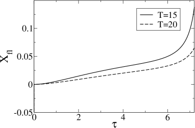
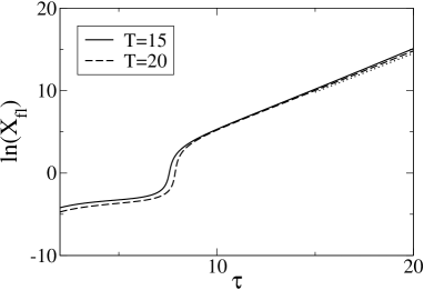
Figure 3: Left: Plot of the fluctuation FDR $X_{\rm fl}$ versus the rescaled time $\tau$, for $d=3$ and $T=15,20$ as shown in the legend. $X_{\rm fl}$ starts off quadratically for small $\tau$, then becomes linear, its slope increasing with decreasing $T$ in both regimes. Eventually it crosses over into a regime of exponential growth, which is not yet visible in the $\tau$-range shown. Right: Plot of $\ln(X_{\rm fl})$ versus $\tau$, at $T=15,20$ as indicated in the legend. This shows the crossover to the regime of $T$-independent exponential increase at large $\tau$, which takes place at $\tau\approx 2\ln T$ and is represented by the dotted line on the right of the graph.

With the expression of the (co-)variances to the required orders at hand, we now plot the contour lines of the joint distribution of the fluctuating correlation and susceptibility $(\hat{C},T\hat{\chi})$. The mean values $C=\langle\hat{C}\rangle$ and $\chi=\langle\hat{\chi}\rangle$ can be read off from (4.5) and (4.7) as $C(\tau)=\exp(-\tau)=1-T\chi(\tau)$ and produce the straight line of slope $-1$ expected from equilibrium FDT. (Note that we do not need to normalize the FD plot because for our local spin correlations the equal time correlator $C(t,t)=1$ always.) Fig. 4 shows contour lines of the fluctuation distributions for a range of different mean values (i.e. different $\tau$); their centres lie on the straight equilibrium FDT line. For the purposes of this graphical illustration, we have aimed to choose a relatively low temperature, as otherwise the covariance becomes too small and all fluctuation contours degenerate into ellipses oriented along the $C$ and $\chi$-axes. We cannot go too low, of course, as otherwise truncating the $1/T$ expansion cannot be justified. The choice $T=10$ is a reasonable compromise: the ${{\mathcal{O}}}(1/T^{2})$ corrections to the variances are then significantly smaller than the leading order terms. However, ${{\mathcal{O}}}(1/T^{3})$ terms – which can be worked out along the lines above – are comparable to the ${{\mathcal{O}}}(1/T^{2})$ contributions, so the results shown are not fully quantitative. We consider $d=3$ and set the scale of the contours by taking $N=50$ and unity for the constant on the RHS of (3.61). The relatively small value of $N$ was taken only for better visibility; a larger value would simply shrink all ellipses uniformly.

 

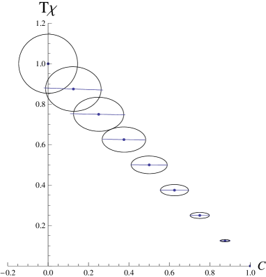
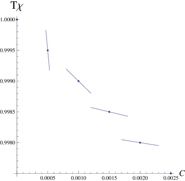
Figure 4: Left: Fluctuations of the coarse-grained local correlation $\hat{C}$ and susceptibility $T\hat{\chi}$ in the high temperature limit. The mean values, indicated by the centres of the ellipses, lie on the straight equilibrium FDT line. The ellipses themselves show contour lines for several different mean values, corresponding to different scaled time differences $\tau=T\Delta t$; we chose $d=3$, $T=10$, $N=50$ and set the constant on the RHS of (3.61) to unity. The principal axis of each ellipse is shown, and represents the direction of the biggest fluctuations. This lies on the correlation axis for small $\tau$ ($X_{\rm fl}\ll 1$) but rotates to lie along the susceptibility axis ($X_{\rm fl}\gg 1$) for large $\tau$. This rotation of the principal axis is continuous but in this graphical representation happens very quickly in the top left corner of the plot: this is because it takes place at large values of $\tau$, i.e. when the mean correlation has already decayed to a very small value. The fluctuation contours in this regime are close to circles and would lie essentially on top of the leftmost ellipse shown. Right: A zoom of the top left corner of the plot on the left. Here only the direction of the principal axis of each ellipse is drawn, to make the rotation towards the $\chi$-axis clearer.

In summary, the fluctuations of correlation and susceptibility are not linked in a manner akin to the equilibrium FDT. The dominant fluctuation direction measured by $X_{\rm fl}$ does not lie on the straight line of slope $-1$ that locates the average quantities. Instead, this direction is along the horizontal (correlation) axis for small times and along the vertical (susceptibility) axis for large times.

4.3 Small time differences

Next we consider the short-time behaviour of the correlation and susceptibility variances at some generic temperature $T\geq T_{\rm c}$. For the correlation one expects from the high-$T$ result that the leading term for small $\Delta t$ will be ${{\mathcal{O}}}(\Delta t^{2})$. We therefore expand $D$ as

$$D = \left[\frac{1}{2}-\frac{T\Delta t}{2}+\frac{K^{\prime\prime}(0)}{16}\Delta t^{2}\right][\delta(t\!-\!t^{\prime})+\delta(t_{\rm w}\!-\!t^{\prime})]+\theta(t^{\prime}\!-\!t_{\rm w})D_{1}+\theta(t_{\rm w}\!-\!t^{\prime})D_{2}$$ (4.27)

$$D_{1} = T-T^{2}\Delta t-\frac{1}{2}L^{(2)}(0)(t-t^{\prime})$$ (4.28)

$$D_{2} = \frac{1}{8}[2TL^{(2)}(t_{\rm w}-t^{\prime})-L^{(2)}{}^{\prime}(t_{\rm w}-t^{\prime})]\Delta t^{2}$$ (4.29)

Here we have used (3.46); $D_{1}$ needs to be expanded only to linear order in quantities of ${{\mathcal{O}}}(\Delta t)$ (including $t-t^{\prime}$) because it is integrated over the range $t_{\rm w}<t^{\prime}<t$ which is itself of ${{\mathcal{O}}}(\Delta t)$. Inserting into (3.41) and expanding the remaining functions (4.8) and (4.10), the various terms involving $L^{(2)}$ cancel to leading order. In fact, to ${{\mathcal{O}}}{(\Delta t^{2})}$, $D_{2}$ only contributes to the single integral in (3.41), where the remaining three-time function $CC$ is set to its zero-order value, and to the double integral when it is combined with the $\delta$-terms appearing in the definition of $D$; however, these contributions cancel. The remaining quantities depending on $L^{(2)}$ are found in $D_{1}$ and are already ${{\mathcal{O}}}{(\Delta t)}$, so they provide contributions of ${{\mathcal{O}}}{(\Delta t^{2})}$ when integrated over $t_{\rm w}<t^{\prime}<t$, if the remaining quantities in the integral are ${{\mathcal{O}}}{(1)}$. Again, this can only be realized in the single integral by setting the three time function $CC$ to its zero order value, and in the coupling with the $\delta$-terms in the double integral, but these terms cancel. Also, in the final result there is a leading order cancellation of the terms proportional to $K^{\prime\prime}(0)$ and one obtains

$$V_{C}(\Delta t)=2T^{2}\Delta t^{2}$$ (4.30)

This agrees in both the $\Delta t$-dependence and the prefactor with the result of the high-$T$ expansion. It is worth noting that in order to get the short time behaviour of the correlation variance, we have expanded $CC(t^{\prime}-t_{\rm w}^{\prime})$ around $CC(0)$. This quantity diverges in $d<4$ at $T=T_{\rm c}$. But the fact that it cancels from the leading short-time behaviour should mean that (4.30) remains valid: in principle we just need to regularize in some way, e.g. by keeping $t_{\rm w}$ large but finite, then perform the short-time expansion and finally remove the regularization, which should lead back to (4.30).

For the susceptibility variance, as given in (3.43), we can expand $D^{\chi}$ as

$$D^{\chi}=\Delta t\,\delta(t-t^{\prime})-\theta(t^{\prime}-t_{\rm w})+{{\mathcal{O}}}(\Delta t)\theta(t^{\prime}-t_{\rm w})+{{\mathcal{O}}}(\Delta t^{2})\theta(t_{\rm w}-t^{\prime})$$ (4.31)

The first two terms and the remainder give contributions of ${{\mathcal{O}}}(\Delta t)$ and ${{\mathcal{O}}}(\Delta t^{2})$ respectively to the integral over $t^{\prime}$. Keeping only the first two terms and replacing $CC(t^{\prime}-t_{\rm w}^{\prime})$ by $CC(0)$ in (3.43) should then give the leading term in $V_{\chi}$ of ${{\mathcal{O}}}(\Delta t^{2})$; but this cancels because $\int dt^{\prime}[\Delta t\,\delta(t-t^{\prime})-\theta(t^{\prime}-t_{\rm w})]=0$. The same argument shows that to ${{\mathcal{O}}}(\Delta t^{3})$ the cross terms between the ${{\mathcal{O}}}(\Delta t)$ and ${{\mathcal{O}}}(\Delta t^{2})$ contributions from (4.31) cancel. The only remaining ${{\mathcal{O}}}(\Delta t^{3})$ term is then

$$V_{\chi} = \frac{1}{2}\int_{t_{\rm w}}^{t}dt^{\prime}dt_{\rm w}^{\prime}[\Delta t\,\delta(t-t^{\prime})-\theta(t^{\prime}-t_{\rm w})][\Delta t\,\delta(t-t_{\rm w}^{\prime})-\theta(t_{\rm w}^{\prime}-t_{\rm w})]CC(t^{\prime}-t_{\rm w}^{\prime})$$ (4.32)

$$= \frac{1}{2}\Delta t^{2}CC(0)-\Delta t\int_{t_{\rm w}}^{t}dt^{\prime}\,CC(t-t^{\prime})+\int_{t_{\rm w}}^{t}dt^{\prime}\int_{t_{\rm w}}^{t^{\prime}}dt_{\rm w}^{\prime}\,CC(t^{\prime}-t_{\rm w}^{\prime})$$ (4.33)

One now expands $CC(t^{\prime}-t_{\rm w}^{\prime})=CC(0)-2T(t^{\prime}-t_{\rm w}^{\prime})$ for $t^{\prime}\geq t_{\rm w}^{\prime}$, using (4.8), to find that the $\Delta t^{2}CC(0)$-terms cancel as expected, leaving

$$V_{\chi}(\Delta t)=\frac{2}{3}T^{3}\Delta t^{3}$$ (4.34)

This again agrees with the high-$T$ expansion in both the scaling with $\Delta t$ and the prefactor.

For the covariance, finally, performing the perturbation expansion in small $\Delta t$ shows that the leading short-time contribution is only of fourth order in $\Delta t$. The temperature dependence of the prefactor is quite complicated and involves the kernel $L^{(2)}$. We only show here the limit of the prefactor for large $T$, which is

$$V_{C\chi}(\Delta t)=-\frac{4dT^{2}}{3}\Delta t^{4}$$ (4.35)

in agreement with (4.22). Correspondingly, the correlation coefficient is again negative, growing in modulus initially as $\gamma\sim-\Delta t^{3/2}$. The fluctuation slope $X_{\rm fl}$ can also be expanded as in the high-$T$ case (4.24), leading again to a quadratic short-time increase

$$X_{\rm fl}\sim-\frac{V_{C\chi}}{V_{C}}\sim\Delta t^{2}$$ (4.36)

4.4 Large time differences

We next turn to the behaviour of the correlation and susceptibility fluctuations at large time differences, at equilibrium at temperatures above criticality; the dynamics at criticality exhibits qualitative differences and is considered separately in the next section. The asymptotic behaviour of (the equilibrium forms of) $K$, $L^{(2)}$ and $CC$ is an exponential decay. For $K$ and $CC$ this follows directly from (4.4) and (4.8), where all Fourier modes decay as $\exp(-2z_{\rm eq}\Delta t)$ or faster. The Laplace transform $\hat{K}(s)$ then has all its singularities bounded away from $s=0$, and the same follows for $\hat{L}^{(2)}(s)$ from (4.11). Thus, looking at $D(t,t_{\rm w},t^{\prime})$ as given by (4.13), the $K(\Delta t/2)$-prefactor ensures that the $\delta$-contributions to $D$ decay exponentially for large time differences, and the same is true for the $D_{1}$-term found in (4.14). The $D_{2}$-term given in (4.15) has the same behaviour. This is obvious for the first term; for the second term, bounding both $K(t)$ and $L^{(2)}(t)$ by $\exp(-ct)$ shows that the integral is bounded by $\Delta t\exp[-c(\bar{t}-t^{\prime})]\leq\Delta t\exp(-c\Delta t/2)$. Thus, for large $\Delta t$, all the non-Gaussian corrections in (3.41), as well as the two-time Gaussian term $CC(t,t_{\rm w})$, decay exponentially to zero; the asymptotic value of the correlation variance is then given by the time-independent Gaussian term $\int(dq)\,C_{\mathbf{q}}(t,t)C_{\mathbf{q}}(t_{\rm w},t_{\rm w})=\int(dq)\,T^{2}/(\omega+z_{\rm eq})^{2}$. This increases as the temperature is reduced towards $T_{\rm c}$; the limit value for $T\to T_{\rm c}$ is finite for $d>4$ but infinite for $d<4$. From the reasoning above it follows that for $T>T_{\rm c}$ the approach of the correlation variance to its asymptotic value for $\Delta t\to\infty$ is exponential in $\Delta t$, up to power law factors.

Analogous reasoning for $D^{\chi}$ in (4.16) leads one to discard as subleading for large $\Delta t$ the $D_{2}^{\chi}$ term in (4.18) and the terms proportional to $K(\Delta t/2)$ appearing in (4.17) for $D_{1}^{\chi}$. The asymptotic susceptibility variance can therefore be found from (3.43) by replacing $D^{\chi}$ with

$$D_{\rm short}^{\chi}=\delta(t-t^{\prime})+\frac{1}{2}K^{\prime}\!\left(\textstyle\frac{t-t^{\prime}}{2}\right)+2TK\!\left(\textstyle\frac{t-t^{\prime}}{2}\right)-\int_{t^{\prime}}^{t}dt^{\prime\prime}\,L^{(2)}(t^{\prime\prime}-t^{\prime})K\!\left(\textstyle\frac{t-t^{\prime\prime}}{2}\right)$$ (4.37)

We have added the subscript “short” because all contributions retained in $D_{\rm short}^{\chi}$ decay exponentially as $t-t^{\prime}$ increases, concentrating the “mass” of the integrals over $t^{\prime}$ and $t_{\rm w}^{\prime}$ in (3.43) into the regions $t-t^{\prime}={{\mathcal{O}}}{(1)}$ and $t-t_{\rm w}^{\prime}={{\mathcal{O}}}{(1)}$. (The factor $CC(t^{\prime}-t_{\rm w}^{\prime})$ does not affect this reasoning as its values are also largest when $t^{\prime}$ is close to $t_{\rm w}^{\prime}$.) Nevertheless, because $CC(t^{\prime}-t_{\rm w}^{\prime})$ does vary significantly on ${{\mathcal{O}}}(1)$ timescales one cannot simplify the expression for the asymptotic value of $V_{\chi}$ further, beyond the replacement of $D^{\chi}$ by $D^{\chi}_{\rm short}$ in (3.43). Barring accidental cancellations (which, by continuity with the nonzero result for $T\to\infty$, one does not expect), the result will be nonzero. The approach to the limit will again be exponential in $\Delta t$.

Finally, in the cross-correlation (3.44) there are no ${{\mathcal{O}}}{(1)}$ contributions that survive in the long-time limit, because every term is proportional to $D$ and thus decays exponentially with $\Delta t$. Qualitatively, then, the behaviour at finite $T>T_{\rm c}$ is the same as that for $T\to\infty$, with the variances of correlation and susceptibility approaching nonzero asymptotic values exponentially fast in $\Delta t$, and the covariance decaying to zero (from below) in the same manner.

5 Quenches to $T_{\rm c}$, $d>4$

Above we derived the large-$N$ statistics of the correlation and susceptibility fluctuations for quenches to temperatures above criticality. In this section and in Sec. 6 we consider quenches directly to criticality, so from now on $T=T_{\rm c}\equiv(\int(dq)\,\,1/\omega)^{-1}$. In principle we then expect aging effects [26, 33], but it will turn out that for the fluctuation statistics these are largely negligible as long as we are in dimension $d>4$. We therefore consider first the situation in equilibrium at criticality in $d>4$, focussing on large time differences $\Delta t$; the short-time limit does not need to be analysed again here because the results in Sec. 4.3 apply even at $T=T_{\rm c}$. As discussed in more detail in Sec. 6, for $d<4$ one has to keep $t_{\rm w}$ finite to avoid the appearance of infinite terms, i.e. one has to look directly at the non-equilibrium situation.

5.1 Equilibrium

The asymptotic behaviour of the equilibrium forms of $K$, $CC$ and $L^{(2)}$ for $T\rightarrow T_{\rm c}$ is quite different from the high temperature phase because $z_{\rm eq}$ vanishes. In the equilibrium form (4.4) of the kernel $K$, the integral is for large time-differences dominated by small $\omega$. Because $\omega\approx q^{2}$ for small $q=|\mathbf{q}|$, the phase space factor in the $\mathbf{q}$-integrals is $(dq)=\sigma_{d}d\omega\,\omega^{d/2-1}$ for small $q$ or $\omega$, with the proportionality constant

$$\sigma_{d}=(4\pi)^{-d/2}\Gamma^{-1}(d/2)$$ (5.1)

Then from (3.15) one finds for large $\Delta t$

$$K(\Delta t)=\sigma_{d}\int d\omega\,\omega^{(d-2)/2}\frac{T}{\omega}e^{-2\omega\Delta t}=k_{d}\Delta t^{(2-d)/2}$$ (5.2)

and correspondingly, from the small-$s$ expansion of (4.11),

$$L^{(2)}(\Delta t)=\lambda_{d}\left\{\begin{array}[]{ll}\Delta t^{(2-d)/2}&\mbox{for $d>4$}\\ \Delta t^{(d-6)/2}&\mbox{for $d<4$}\end{array}\right.$$ (5.3)

with $k_{d}$ and $\lambda_{d}$ $d$-dependent constants [33].

In equilibrium at criticality the function $CC(\Delta t)$ also decays as a power law for $\Delta t\gg 1$. This can easily be worked out in $d>4$:

$$CC(\Delta t)=\int(dq)\,\frac{T^{2}}{\omega^{2}}e^{-2\omega\Delta t}=2T\int_{\Delta t}^{\infty}dt^{\prime}\,K(t^{\prime})\sim\Delta t^{(4-d)/2}$$ (5.4)

The three-time function $CC(t,t_{\rm w},t^{\prime})$ given in (4.10) increases with $t^{\prime}$ up to $t^{\prime}=t_{\rm w}$; in the range $t^{\prime}=t_{\rm w}\ldots t$ it then remains constant and equal to $CC(\Delta t/2)$.

For the correlation variance (3.41), the first of the two Gaussian terms is a constant of order unity, $\int(dq)\,C_{\mathbf{q}}(t,t)C_{\mathbf{q}}(t_{\rm w},t_{\rm w})=\int(dq)\,T^{2}/\omega^{2}$. The second one, $CC(\Delta t)$, is proportional to $\Delta t^{(4-d)/2}$ for large $\Delta t$ from (5.4). One can show that these are in fact the two leading terms, with the non-Gaussian corrections contributing at most ${{\mathcal{O}}}(\Delta t^{4-d})$ asymptotically. (See [42] for a detailed discussion of the scaling of these terms.) Note that because the prefactor of $CC(\Delta t)\sim\Delta t^{(4-d)/2}$ in (3.41) is positive, $V_{C}$ approaches its (positive) asymptotic value from above; given that it starts at zero at $\Delta t=0$, it is therefore non-monotonic in $\Delta t$. Because $V_{C}(\Delta t)$ must depend continuously on temperature, at least at finite $\Delta t$, this non-monotonicity must then be present also in a range of temperatures above $T_{\rm c}$.

To understand the asymptotics of the susceptibility variance (3.43) it is useful to decompose

$$D^{\chi}(t,t_{\rm w},t^{\prime})=D^{\chi}_{\rm short}(t,t_{\rm w},t^{\prime})+D^{\chi}_{\rm long}(t,t_{\rm w},t^{\prime})$$ (5.5)

where

$$D^{\chi}_{\rm long}(t,t_{\rm w},t^{\prime})=-K\!\left(\textstyle\frac{\Delta t}{2}\right)\delta(t-t^{\prime})\!+\!D^{\chi}_{1,\rm long}(t,t_{\rm w},t^{\prime})\theta(t^{\prime}-t_{\rm w})\!+\!D_{2}^{\chi}(t,t_{\rm w},t^{\prime})\theta(t_{\rm w}-t^{\prime})$$ (5.6)

and

$$D^{\chi}_{1,\rm long}(t,t_{\rm w},t^{\prime})=-K\!\left(\textstyle\frac{\Delta t}{2}\right)\left[2T-\int_{t^{\prime}}^{t}dt^{\prime\prime}\,L^{(2)}(t^{\prime\prime}-t^{\prime})\right]$$ (5.7)

while $D^{\chi}_{2}$ is as written in (4.18). The short-time part of (5.5), defined in (4.37), decays on timescales $t-t^{\prime}={{\mathcal{O}}}(1)$ and its integral over $t^{\prime}$ is of order unity. More precisely, Laplace transforming $D^{\chi}_{\rm short}(t,t_{\rm w},t^{\prime})$ w.r.t. $t-t^{\prime}$ and expanding for small $s$ gives

$$\hat{D}_{\rm short}^{\chi}(s) = 2\hat{K}(2s)[s+2T-\hat{L}(s)]=2\frac{\hat{K}(2s)}{\hat{K}(s)}\approx 2\frac{\hat{K}(0)-c(2s)^{(d-4)/2}}{\hat{K}(0)-cs^{(d-4)/2}}$$ (5.8)

$$\approx 2+2\frac{c}{\hat{K}(0)}s^{(d-4)/2}(1-2^{(d-4)/2})$$ (5.9)

where we used (4.11) and the small $s$-expansion of $\hat{K}(s)=\hat{K}(0)-cs^{(d-4)/2}$ [33]. This shows that the integral of $D^{\chi}_{\rm short}(t-t^{\prime})$ over all $t-t^{\prime}$ equals 2, and that $D^{\chi}_{\rm short}(t-t^{\prime})$ decays as $(t-t^{\prime})^{(2-d)/2}$ for large $\Delta t$. The complementary long-time part $D^{\chi}_{\rm long}$, on the other hand, can be seen to have a structure similar to that of $D$: the $\delta$-term has weight $\sim\Delta t^{(2-d)/2}$, $D^{\chi}_{1,\rm long}$ is of order $\Delta t^{(2-d)/2}$ (and constant for $t-t^{\prime}\gg 1$), and $D^{\chi}_{2}$ is of order $L^{(2)}(t-t^{\prime})\sim(t-t^{\prime})^{(2-d)/2}$. Decomposing now the product $D^{\chi}D^{\chi}$ in (3.43) according to (5.5), the $D^{\chi}_{\rm short}D^{\chi}_{\rm short}$ term gives the leading asymptotic term of $V_{\chi}$, a constant of order unity. We omit here the detailed analysis of the scaling of the other terms, which can be found in [42], and point out only that overall $V_{\chi}$ approaches its asymptotic value via leading power law terms $\sim\Delta t^{(2-d)/2}$ and $\sim\Delta t^{4-d}$; the former dominates for $d>6$, the latter for $4<d<6$. There appears to be no simple way of estimating the sign of these terms to verify whether $V_{\chi}$, like $V_{C}$, has a non-monotonic $\Delta t$-dependence.

In the covariance (3.44) there are, as in the case of $T>T_{\rm c}$, no ${{\mathcal{O}}}{(1)}$ terms that survive for long times. To obtain the leading decay to zero, one considers first the single integral involving $D^{\chi}$ and the three-time function $CC(t,t_{\rm w},t^{\prime})$. The leading contribution arises from the short-time part $D^{\chi}_{\rm short}$ of $D^{\chi}$, giving $\approx-2CC(t,t_{\rm w},t)=-2CC(t-t_{\rm w})\sim-\Delta t^{(4-d)/2}$, so that $V_{C\chi}(\Delta t)$ approaches $0$ from below as $-\Delta t^{(4-d)/2}$. The scaling of the remaining subleading terms is analysed in [42].

A schematic plot of the full $\Delta t$-dependence of the variances and the covariance at criticality and $d>4$ is shown in Fig. 5. The non-monotonicity of the correlation variance (and, possibly, the susceptibility variance) is consistent with a scenario in which for both short and long time regimes local correlations and responses display minor fluctuations across the system and dynamical histories, whereas for intermediate time they depend strongly on the particular state reached by the system in a given time interval, making fluctuations across dynamical histories large. This type of behaviour is quite generic: indeed, as explained after (2.4), $V_{C}$ is the four-point function commonly used to quantify dynamic heterogeneities, and this is found to exhibit a maximum as a function of $\Delta t$ for many systems with slow dynamics [10, 11, 14]. Note though that typically (e.g. in coarsening below $T_{\rm c}$ [23, 24]) the position of the maximum scales with the age of the system whereas here, for coarsening at criticality above the upper critical dimension, it occurs for an age-independent time difference $\Delta t$.

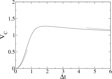
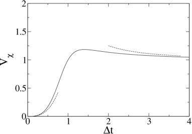
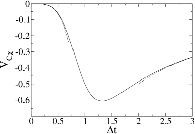
Figure 5: Schematic plot of the $\Delta t$-dependence of the variances, $V_{C}$ and $V_{\chi}$, and covariance, $V_{C\chi}$, for critical coarsening and $d>4$. These functions increase from $0$ to ${{\mathcal{O}}}{(1)}$ values as power laws of $\Delta t$ given respectively in (4.30), (4.34) and (4.35), and then decay asymptotically with negative powers of $\Delta t$. $V_{C}$ and $V_{C\chi}$ are non-monotonic; for $V_{\chi}$ it is not obvious whether the asymptotic value is approached from above or below.

Gathering the above results for $\Delta t\rightarrow\infty$, $V_{C}(\Delta t)\rightarrow{{\mathcal{O}}}{(1)}$, $V_{\chi}(\Delta t)\rightarrow{{\mathcal{O}}}{(1)}$ and $V_{C\chi}(\Delta t)\rightarrow-\Delta t^{(4-d)/2}$, yields for the correlation coefficient the power law decrease $\gamma\sim-\Delta t^{(4-d)/2}$. The FDR for the local fluctuations $X_{\rm fl}$ as given in (3.62) is then positive, but to say more one would need to know whether $V_{C}$ and $V_{\chi}$ is bigger for $\Delta t\to\infty$. If $V_{C}>V_{\chi}$, the elliptical contour of $P(\hat{C},T\hat{\chi})$ has its main axis along the $\hat{C}$ direction and, as one can show formally by expanding (3.62) for small $\gamma$, $X_{\rm fl}\sim-\gamma\sim\Delta t^{(4-d)/2}$ decays to zero. Conversely, if $V_{\chi}>V_{C}$ the main axis of the ellipse is along the $\hat{\chi}$ direction and the fluctuation slope $X_{\rm fl}\sim-1/\gamma\sim\Delta t^{(d-4)/2}$ becomes vertical for $\Delta t\to\infty$. In the limiting case where $V_{C}$ and $V_{\chi}$ are equal asymptotically, $(V_{C}/V_{\chi})^{1/2}-(V_{\chi}/V_{C})^{1/2}$ in (3.62) would decay as $\Delta t^{(4-d)/2}$, being controlled by the leading corrections to $V_{C}$; because this is proportional to $\gamma$, a finite asymptotic value of $X_{\rm fl}$ would result. From the high-$T$ expansion of Sec. 4.2 one can see that at order $1/T^{2}$, differences between the asymptotic values of $V_{C}$ and $V_{\chi}$ appear. These suggest that the scenario that should apply is the one where $V_{\chi}>V_{C}$ asymptotically and therefore the main axis of the fluctuation ellipse is along the $\hat{\chi}$ direction.

5.2 Non-equilibrium, $d>4$

Now we study the behaviour of correlation and susceptibility fluctuations for the genuine out-of-equilibrium dynamics after a quench to criticality, focussing on $d>4$ as in the previous subsection. Here we get correction factors with respect to the equilibrium case which become important in the aging regime, $t-t_{\rm w}\sim t_{\rm w}$. More precisely, aging effects appear in the long time ($t,t_{\rm w}\gg 1$) behaviour of two-time functions via scaling functions of the time ratio $t/t_{\rm w}$ that modulate the equilibrium part, e.g.

$$K(t,t_{\rm w})=K_{\rm eq}(t-t_{\rm w}){\mathcal{F}}_{K}\!\left(\textstyle\frac{t}{t_{\rm w}}\right)$$ (5.10)

$$L^{(2)}(t,t_{\rm w})=L^{(2)}_{\rm eq}(t-t_{\rm w}){\mathcal{F}}_{L}\!\left(\textstyle\frac{t}{t_{\rm w}}\right)$$ (5.11)

with ${\mathcal{F}}_{K}(1)={\mathcal{F}}_{L}(1)=1$ [33]. Here and throughout the remainder of the paper we distinguish the TTI equilibrium contributions with the subscript “eq”. The two-time correlation $C(t,t_{\rm w})$ has a similar scaling behaviour as can be seen by expressing it in terms of the kernel $K$:

$$C(t,t_{\rm w}) = \int(dq)\,R_{\mathbf{q}}(t,t_{\rm w})C_{\mathbf{q}}(t_{\rm w},t_{\rm w})=\sqrt{\frac{g(t_{\rm w})}{g(t)}}\int(dq)\,e^{-\omega(t-t_{\rm w})}C_{\mathbf{q}}(t_{\rm w},t_{\rm w})$$ (5.12)

$$= \frac{g(\bar{t})}{\sqrt{g(t)g(t_{\rm w})}}K(\bar{t},t_{\rm w})=K_{\rm eq}\!\left(\textstyle\frac{\Delta t}{2}\right)\frac{g(\bar{t})}{\sqrt{{g(t)}g(t_{\rm w})}}{\mathcal{F}}_{K}\!\left(\textstyle\frac{\bar{t}}{t_{\rm w}}\right)$$ (5.13)

The long-time behaviour of the function $D$ from (3.40) that defines the correlation variance is thus given by (using  (3.47), (3.48) and (3.50))

$$D(t,t_{\rm w},t^{\prime}) = \frac{1}{2}K_{\rm eq}\!\left(\textstyle\frac{\Delta t}{2}\right)\frac{g(\bar{t})}{\sqrt{{g(t)}g(t_{\rm w})}}{\mathcal{F}}_{K}\!\left(\textstyle\frac{x+1}{2}\right)[\delta(t-t^{\prime})+\delta(t_{\rm w}-t^{\prime})]$$ (5.14)

$${}+D_{1}(t,t_{\rm w},t^{\prime})\theta(t^{\prime}-t_{\rm w})+D_{2}(t,t_{\rm w},t^{\prime})\theta(t_{\rm w}-t^{\prime})$$

where $x=t/t_{\rm w}$ and

$$D_{1}(t,t_{\rm w},t^{\prime})=\frac{1}{2}K_{\rm eq}\!\left(\textstyle\frac{\Delta t}{2}\right)\frac{g(\bar{t})}{\sqrt{{g(t)}g(t_{\rm w})}}{\mathcal{F}}_{K}\!\left(\textstyle\frac{x+1}{2}\right)\left[2T-\int_{t^{\prime}}^{t}d\tau\,L^{(2)}_{\rm eq}(\tau-t^{\prime}){\mathcal{F}}_{L}\!\left(\textstyle\frac{\tau}{t^{\prime}}\right)\right]$$ (5.15)

and

$$D_{2}(t,t_{\rm w},t^{\prime}) = -\frac{1}{2}K_{\rm eq}\!\left(\textstyle\frac{\Delta t}{2}\right)\frac{g(\bar{t})}{\sqrt{{g(t)}g(t_{\rm w})}}{\mathcal{F}}_{K}\!\left(\textstyle\frac{x+1}{2}\right)\int_{t_{\rm w}}^{t}d\tau\,L_{\rm eq}^{(2)}(\tau-t^{\prime}){\mathcal{F}}_{L}\!\left(\textstyle\frac{\tau}{t^{\prime}}\right)$$ (5.16)

$${}+\frac{g(\bar{t})}{\sqrt{g(t)g(t_{\rm w})}}\int_{t_{\rm w}}^{\bar{t}}d\tau\,K_{\rm eq}\!\left(\textstyle\bar{t}-\tau\right){\mathcal{F}}_{K}\!\left(\textstyle\frac{\bar{t}}{\tau}\right)L_{\rm eq}^{(2)}(\tau-t^{\prime}){\mathcal{F}}_{L}\!\left(\textstyle\frac{\tau}{t^{\prime}}\right)$$

For $d>4$ and long times $g(t)\sim{\rm const}$ and all the factors involving $g(t)$ in the above expressions can be dropped.

In order to get the long-time expression for $D^{\chi}$ from (3.52) we need the non-equilibrium form of $\chi(t,t_{\rm w})$. In equilibrium, $1-T\chi_{\rm eq}(\Delta t)=K_{\rm eq}(\Delta t/2)$ and so we consider the same combination here:

$$1-T\chi(t,t_{\rm w})=1-T\int(dq)\,\int_{t_{\rm w}}^{t}dt^{\prime}\,e^{-\omega(t-t^{\prime})}\sqrt{\frac{g(t^{\prime})}{g(t)}}$$ (5.17)

This can be rewritten, by adding and subtracting the quantity $T\int(dq)\,\int_{t_{\rm w}}^{t}dt^{\prime}\,e^{-\omega(t-t^{\prime})}=1-K_{\rm eq}(\Delta t/2)$, as

$$1-T\chi(t,t_{\rm w})=K_{\rm eq}\left(\textstyle\frac{\Delta t}{2}\right)-T\int(dq)\,\int_{t_{\rm w}}^{t}dt^{\prime}\,e^{\omega(t-t^{\prime})}\left(\sqrt{\frac{g(t^{\prime})}{g(t)}}-1\right)$$ (5.18)

and extracting a factor of $K_{\rm eq}(\Delta t/2)$ from the second term yields

$$1-T\chi(t,t_{\rm w})=K_{\rm eq}\!\left(\textstyle\frac{\Delta t}{2}\right){\mathcal{F}}_{\chi}(x)$$ (5.19)

Bearing in mind that $\int(dq)\,e^{-\omega(t-t^{\prime})}=-K_{\rm eq}^{\prime}(t-t^{\prime})/(2T)$ the aging function ${\mathcal{F}}_{\chi}$ can be written as

$${\mathcal{F}}_{\chi}(x) = 1+\frac{1}{2}\frac{\int_{t_{\rm w}}^{t}dt^{\prime}\,K_{\rm eq}^{\prime}\left(\textstyle\frac{t-t^{\prime}}{2}\right)\left(\sqrt{\frac{g(t^{\prime})}{g(t)}}-1\right)}{K_{\rm eq}(\Delta t/2)}$$ (5.20)

Because $g(t)$ approaches a constant for large times in $d>4$, the integral term in fact vanishes in the limit and there is no aging correction: ${\mathcal{F}}_{\chi}(x)=1$. Inserting (5.19) into (3.52), (3.53) and (3.54) one finds the long-time non-equilibrium form of $D^{\chi}$

$$D^{\chi}(t,t_{\rm w},t^{\prime}) = \left[1\!-\!K_{\rm eq}\!\left(\textstyle{\frac{\Delta t}{2}}\right){\mathcal{F}}_{\chi}(x)\right]\delta(t-t^{\prime})$$ (5.21)

$$\!+\!D_{1}^{\chi}(t,t_{\rm w},t^{\prime})\theta(t^{\prime}-t_{\rm w})\!+\!D_{2}^{\chi}(t,t_{\rm w},t^{\prime})\theta(t_{\rm w}-t^{\prime})$$

with

$$D_{1}^{\chi}(t,t_{\rm w},t^{\prime}) = \frac{1}{2}K^{\prime}_{\rm eq}\!\left(\textstyle\frac{t-t^{\prime}}{2}\right){\mathcal{F}}_{\chi}\!\left(\textstyle\frac{t}{t^{\prime}}\right)+\frac{t}{t^{\prime 2}}K_{\rm eq}\!\left(\textstyle\frac{t-t^{\prime}}{2}\right){\mathcal{F}}_{\chi}^{\prime}\!\left(\textstyle\frac{t}{t^{\prime}}\right)$$ (5.22)

$${}+2T\left[K_{\rm eq}\!\left(\textstyle\frac{t-t^{\prime}}{2}\right){\mathcal{F}}_{\chi}(\textstyle\frac{t}{t^{\prime}})-K_{\rm eq}\!\left({\textstyle\frac{\Delta t}{2}}\right){\mathcal{F}}_{\chi}(x)\right]$$

$${}-\int_{t^{\prime}}^{t}dt^{\prime\prime}\,L_{\rm eq}^{(2)}(t^{\prime\prime}-t^{\prime}){\mathcal{F}}_{L}(\textstyle\frac{t^{\prime\prime}}{t^{\prime}})\left[K_{\rm eq}\!\left(\textstyle\frac{t-t^{\prime\prime}}{2}\right){\mathcal{F}}_{\chi}(\textstyle\frac{t}{t^{\prime\prime}})-K_{\rm eq}\!\left(\textstyle\frac{\Delta t}{2}\right){\mathcal{F}}_{\chi}(x)\right]$$

and

$$D_{2}^{\chi}(t,t_{\rm w},t^{\prime})=-\int_{t_{\rm w}}^{t}dt^{\prime\prime}\,L_{\rm eq}^{(2)}(t^{\prime\prime}-t^{\prime}){\mathcal{F}}_{L}(\textstyle\frac{t^{\prime\prime}}{t^{\prime}})\left[K_{\rm eq}\!\left(\textstyle\frac{t-t^{\prime\prime}}{2}\right){\mathcal{F}}_{\chi}(\textstyle\frac{t}{t^{\prime\prime}})-K_{\rm eq}\!\left(\textstyle\frac{\Delta t}{2}\right){\mathcal{F}}_{\chi}(x)\right]$$ (5.23)

It will be useful to separate short and long time parts in $D^{\chi}$ again:

$$D^{\chi}(t,t_{\rm w},t^{\prime})=D^{\chi}_{\rm short}(t,t_{\rm w},t^{\prime})+D^{\chi}_{\rm long}(t,t_{\rm w},t^{\prime})$$ (5.24)

We arrange the terms so that the first term is identical to its equilibrium counterpart (4.37) except for a slowly varying aging correction, giving

$$D_{\rm short}^{\chi}(t,t_{\rm w},t^{\prime}) = {\mathcal{F}}_{\chi}\!\left(\textstyle\frac{t}{t^{\prime}}\right)\biggl{[}\delta(t-t^{\prime})+\frac{1}{2}K^{\prime}_{\rm eq}\!\left(\textstyle\frac{t-t^{\prime}}{2}\right)+2TK_{\rm eq}\!\left(\textstyle\frac{t-t^{\prime}}{2}\right)$$ (5.25)

$${}-\int_{t^{\prime}}^{t}dt^{\prime\prime}\,L_{\rm eq}^{(2)}(t^{\prime\prime}-t^{\prime})K_{\rm eq}\!\left(\textstyle\frac{t-t^{\prime\prime}}{2}\right)\biggr{]}\theta(t^{\prime}-t_{\rm w})$$

$$D^{\chi}_{\rm long}(t,t_{\rm w},t^{\prime}) = {}-K\!\left(\textstyle\frac{\Delta t}{2}\right){\mathcal{F}}_{\chi}(x)\delta(t-t^{\prime})+D^{\chi}_{1,\rm long}(t,t_{\rm w},t^{\prime})\theta(t^{\prime}-t_{\rm w})\!$$ (5.26)

$${}+\!D_{2}^{\chi}(t,t_{\rm w},t^{\prime})\theta(t_{\rm w}-t^{\prime})$$

$$D_{1,\rm long}^{\chi}(t,t_{\rm w},t^{\prime}) = \frac{t}{t^{\prime 2}}K_{\rm eq}\!\left(\textstyle\frac{t-t^{\prime}}{2}\right){\mathcal{F}}_{\chi}^{\prime}\!\left(\textstyle\frac{t}{t^{\prime}}\right)-K_{\rm eq}\!\left(\textstyle\frac{\Delta t}{2}\right)\!{\mathcal{F}}_{\chi}(x)\!\left[2T-\int_{t^{\prime}}^{t}dt^{\prime\prime}\,L_{\rm eq}^{(2)}(t^{\prime\prime}\!-\!t^{\prime}){\mathcal{F}}_{L}\!\left(\textstyle\frac{t^{\prime\prime}}{t^{\prime}}\right)\right]$$ (5.27)

$${}-\int_{t^{\prime}}^{t}dt^{\prime\prime}\,L_{\rm eq}^{(2)}(t^{\prime\prime}-t^{\prime})K_{\rm eq}\!\left(\textstyle\frac{t-t^{\prime\prime}}{2}\right)\left[{\mathcal{F}}_{L}\!\left(\textstyle\frac{t^{\prime\prime}}{t^{\prime}}\right){\mathcal{F}}_{\chi}\!\left(\textstyle\frac{t}{t^{\prime\prime}}\right)-{\mathcal{F}}_{\chi}\!\left(\textstyle\frac{t}{t^{\prime}}\right)\right]$$

We have kept the factors of ${\mathcal{F}}_{\chi}$ so that the expressions are valid also in $d<4$, for later use. For our current case ($d>4$), one has ${\mathcal{F}}_{\chi}=1$ and ${\mathcal{F}}_{\chi}^{\prime}=0$.

To deduce the behaviour of $V_{C}$, $V_{\chi}$ and $V_{C\chi}$ we finally need the aging corrections to the function $CC$ defined in (3.37), (3.38). One uses (3.10) and the long-time scaling of the equal-time correlator $C_{\mathbf{q}}(t_{\rm w},t_{\rm w})=(T/\omega){\mathcal{F}}_{C}(\omega t_{\rm w})$ with ${\mathcal{F}}_{C}(w)\rightarrow 1$ for $w\rightarrow\infty$ and ${\mathcal{F}}_{C}(w)\approx 2w$ for $w\rightarrow 0$; in $d>4$, ${\mathcal{F}}_{C}(w)=1-\exp(-2w)$ [33]. The ratio of the three-time function to its equilibrium counterpart is then, for $t^{\prime}>t_{\rm w}$,

$$\frac{CC(t,t_{\rm w},t^{\prime})}{CC_{\rm eq}(t,t_{\rm w},t^{\prime})}=\frac{\int(dq)\,(T^{2}/\omega^{2}){\mathcal{F}}_{C}(\omega t^{\prime}){\mathcal{F}}_{C}(\omega t_{\rm w})e^{-\omega(t-t_{\rm w})}}{\int(dq)\,(T^{2}/\omega^{2})e^{-\omega(t-t_{\rm w})}}$$ (5.28)

In the aging regime where $t-t_{\rm w}\gg 1$ and so only $\omega\ll 1$ contributes one can replace $(dq)\sim d\omega\,\omega^{d/2-1}$; rescaling $\omega$ to $w=\omega t_{\rm w}$ then gives a function of $x=t/t_{\rm w}$ and $y=t^{\prime}/t_{\rm w}$:

$$\frac{CC(t,t_{\rm w},t^{\prime})}{CC_{\rm eq}(t,t_{\rm w},t^{\prime})}={\mathcal{F}}_{CC}(x,y),\quad{\mathcal{F}}_{CC}(x,y)=\frac{\int dw\,w^{(d-6)/2}{\mathcal{F}}_{C}(wy){\mathcal{F}}_{C}(w)e^{-w(x-1)}}{\int dw\,w^{(d-6)/2}e^{-w(x-1)}}$$ (5.29)

With the same approach one finds for $t^{\prime}<t_{\rm w}$, i.e. $y<1$,

$${\mathcal{F}}_{CC}(x,y)=\frac{\int dw\,w^{(d-6)/2}{\mathcal{F}}_{C}^{2}(wy)e^{-w(x+1-2y)}}{\int dw\,w^{(d-6)/2}e^{-w(x+1-2y)}}$$ (5.30)

The function ${\mathcal{F}}_{CC}$ also governs the aging corrections for the two-time $CC$, according to

$$\frac{CC(t,t_{\rm w})}{CC_{\rm eq}(t-t_{\rm w})}=\frac{CC(t,t,t_{\rm w})}{CC_{\rm eq}(t,t,t_{\rm w})}={\mathcal{F}}_{CC}(1,1/x)$$ (5.31)

We can now proceed to study what, if any, aging corrections there are for the correlation and susceptibility (co-)variances in $d>4$. The scaling functions ${\mathcal{F}}_{K}$, ${\mathcal{F}}_{L}$, ${\mathcal{F}}_{\chi}$, ${\mathcal{F}}_{CC}$ are all bounded by $1$. One can check that the presence of the aging corrections in $D$ and $D^{\chi}$ does not increase the order of the various terms and that the asymptotic values of $V_{C}$ and $V_{\chi}$ are identical to the ones in equilibrium, with aging corrections visible only very weakly in the decay to these asymptotes. A detailed discussion of the effects of aging corrections on $V_{C}$ and $V_{\chi}$ is provided in [42]. Here we mention only that the leading correction to the asymptotic value of $V_{C}$ displays a crossover from the value $CC_{\rm eq}(t-t_{\rm w})$, obtained in the near equilibrium regime $x\approx 1$ (where ${\mathcal{F}}_{CC}(1,1/x)\approx 1$), to an $x$-independent negative constant of order $t_{\rm w}^{(4-d)/2}$ for $x\gg 1$. This negative contribution provides a small downward shift in the value of $V_{C}$ that is reached asymptotically, as $t$ becomes large ($t\gg t_{\rm w}$) at fixed $t_{\rm w}$.

The only significant aging effect in critical coarsening for $d>4$ is visible in the covariance, whose leading term can be shown to be [42] $V_{C\chi}=-2CC_{\rm eq}(\Delta t/2){\mathcal{F}}_{CC}(x,x)\sim-t_{\rm w}^{(4-d)/2}(x-1)^{(4-d)/2}{\mathcal{F}}_{CC}(x,x)$, that is the equilibrium result supplemented with an aging correction ${\mathcal{F}}_{CC}(x,x)$. For $x\approx 1$ the latter equals one as it should to reproduce the equilibrium result; for large $x$, one finds from (5.29) that ${\mathcal{F}}_{CC}(x,y)\sim y/x^{2}$ and so ${\mathcal{F}}_{CC}(x,x)\sim 1/x$.

6 Quenches to $T_{\rm c}$, $d<4$

In this section we will study the fluctuations in the out-of-equilibrium dynamics of the spherical ferromagnet quenched to criticality in dimension $d<4$. Here we cannot start from an equilibrium calculation and later account for aging corrections because a naive equilibrium limit leads to the appearance of infinite terms: in the correlation variance (3.41), for example, the first Gaussian term becomes $\int(dq)\,T^{2}/\omega^{2}$ for $t,t_{\rm w}\to\infty$ which is infinite in $d<4$. Thus, we need to look directly at the non-equilibrium situation. Specifically, we will consider the aging limit $t,t_{\rm w}\to\infty$ but at fixed $x=t/t_{\rm w}>1$. We omit the calculations for this scenario as they are somewhat technical; the interested reader can find full derivations in Ref. [42].

Our analysis shows that in the aging regime the variances and the covariance all scale as $t_{\rm w}^{(4-d)/2}$ times a function of $x$. The dependence on $x$ implies that the relevant timescale on which the (co-)variances vary is $\Delta t\sim t_{\rm w}$, in contrast to the case $d>4$ where this timescale is $\Delta t={{\mathcal{O}}}(1)$ independently of the age $t_{\rm w}$. In this sense the behaviour for $d<4$ is similar to what is seen for coarsening (in general $d$) at $T<T_{\rm c}$ [23, 24]. Interestingly, however, the amplitude of the (co-)variances grows with the age $t_{\rm w}$ only as $t_{\rm w}^{(4-d)/2}$ at criticality, whereas below $T_{\rm c}$ it scales (at least for $V_{C}$) in the naive way as the domain volume $\sim(t_{\rm w}^{1/2})^{d}$.

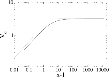
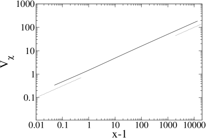
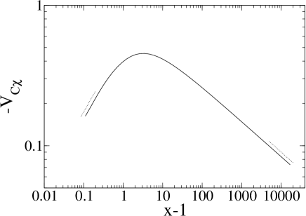
Figure 6: Log-log plots of correlation and susceptibility variances $V_{C}$ (top left), $V_{\chi}$ (top right) and covariance $V_{C\chi}$ (bottom) versus $x-1=(t-t_{\rm w})/t_{\rm w}$, for critical coarsening in dimension $d=3$. As in all following figures, the (co-)variances have been divided by $t_{\rm w}^{(4-d)/2}$ to get functions of $x$ only. The theoretically expected power laws for large $x$ are given, respectively, by $V_{C}\sim x^{0}$, $V_{\chi}\sim x^{(4-d)/2}$ and $V_{C\chi}\sim-x^{2-3d/4}$ and are represented by the dotted lines on the right of each graph. The ${{\mathcal{O}}}{(1)}$ value approached by the correlation variance is represented by the Gaussian term and it can be calculated analytically [42]; this value is represented by the horizontal dotted line in the first graph. The initial increase $\sim(x-1)^{(4-d)/2}$ for all three quantities is indicated similarly on the left. Note that for $V_{\chi}$ the initial and asymptotic power laws are identical, so that the log-log plot overall is close to linear.

The dependence on $x$ of the (co-)variances can be evaluated numerically from the scaling expressions for the aging limit; the results are shown in Fig. 6 for $d=3$. We also study numerically the $x$-dependence of the resulting correlation coefficient $\gamma$ and the fluctuation slope $X_{\rm fl}$, as displayed in Fig. 7. In both of these quantities the $t_{\rm w}^{(4-d)/2}$ prefactor from the (co-)variances cancels, so they depend solely on $x$.

  

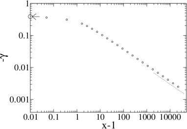
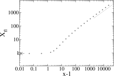
Figure 7: Log-log plot of the absolute value of the correlation coefficient $\gamma$ (left) and the fluctuation slope $X_{\rm fl}$ (right) versus $x-1=(t-t_{\rm w})/t_{\rm w}$ for critical coarsening in $d=3$. The modulus of the correlation coefficient $\gamma$ is always smaller than $1$, as it should be. For large $x$, $\gamma$ decays as $-x^{(2-d)/2}$, as shown by the dotted line on the right of the plot. The separately calculated limit value for $x\rightarrow 1$ is indicated by the arrow on the $y$-axis and is certainly plausible as an asymptote for $\ln(x-1)\to-\infty$ of our numerics for $x$ close to 1. The fluctuation slope $X_{\rm fl}$ behaves for large $x$ as $x^{d/4}$. This predicted power law is represented by the dotted line on the right, while the value that should be approached for $x\rightarrow 1$ is indicated by the arrow on the $y$-axis.

Figure 8: Left: The prefactors of the (co-)variances in the TTI regime $x=t/t_{\rm w}\approx 1$, where they are proportional to $(t-t_{\rm w})^{(4-d)/2}$, are plotted versus $d$. All three prefactors diverge as $1/(4-d)$ for $d$ close to $4$ and vanish as power laws for $d$ near $2$, specifically $\nu_{C}\sim(d-2)^{2}$ and $\nu_{\chi}\sim\nu_{C\chi}\sim(d-2)^{3}$. Right: Plot of the prefactors normalised by their predicted limiting behaviour as $\delta=(4-d)/2\to 0$ [42], $16\pi^{2}\delta\nu_{C}/(3T_{\rm c}^{2})$, $4\pi^{2}\delta\nu_{\chi}/T_{\rm c}^{2}$ and $-8\pi^{2}\delta\nu_{C\chi}/T_{\rm c}^{2}$, versus $d$. The inset shows the correlation variance prefactor normalized by its predicted limiting behaviour as $\delta^{\prime}=(d-2)/2\to 0$.

Figure 9: Correlation coefficient $\gamma$ and fluctuation slope $X_{\rm fl}$ for $x=t/t_{\rm w}\rightarrow 1$, plotted versus $d$. The circles show the limits of $\gamma$ and $X_{\rm fl}$ for $d\rightarrow 4$, calculated analytically and given respectively by $-1/\sqrt{3}$ and $(1+\sqrt{17})/4$ (see [42]). The inset on the left shows the correlation coefficient normalized by its predicted power law as it approaches $d=2$. The loss of accuracy around $d=2$ is due to numerical inaccuracies in the evaluation of the correlation variance as $d$ gets very close to $2$ [42].

One can analyse the behaviour of the quantities above in more detail for the two opposite extremes $\epsilon=x-1\ll 1$ and $x\gg 1$. In the former case we expect to recover quasi-equilibrium behaviour with all dependences being only on time differences. One can show by an expansion in $\epsilon$ [42] that indeed the (co-)variances all grow as $\epsilon^{(4-d)/2}$ to leading order; combining this with the overall $t_{\rm w}^{(4-d)/2}$ scaling, one gets a TTI time dependence as expected, proportional to $(t-t_{\rm w})^{(4-d)/2}$. The prefactors $\nu_{C}$, $\nu_{\chi}$ and $\nu_{C\chi}$ of this power law increase in $V_{C}$, $V_{\chi}$ and $V_{C\chi}$ are plotted as functions of dimensionality in Fig. 8. Given that $V_{C}$, $V_{\chi}$, $V_{C\chi}$ all have the same scaling with $t-t_{\rm w}$ in this regime, the correlation coefficient and fluctuation slope also have nontrivial values; these are plotted against $d$ in Fig. 9. Note that because we are approaching the TTI regime via the limit $x\to 1$ of an aging calculation, where $t-t_{\rm w}\sim t_{\rm w}\gg 1$ always, these results are valid for $t-t_{\rm w}\gg 1$ only. For $t-t_{\rm w}\ll 1$, on the other hand, the results of Sec. 4.3 will apply and both $\gamma$ and $X_{\rm fl}$ will tend to zero in the limit $t\to t_{\rm w}$. If we were to plot the contour lines of the distribution of $(\hat{C},T\hat{\chi})$ on an FD plot the initial section (bottom right) would therefore look similar to Fig. 4, but then the ellipses would grow as $(t-t_{\rm w})^{(4-d)/2}$ as the top left hand corner of the plot is approached and their principal axis would approach a limiting slope given by $X_{\rm fl}$ in Fig. 9 as a function of $d$. The genuine aging effects occurring for $x>1$ would not be visible because they are all compressed into the top left corner of the plot in the limit $t_{\rm w}\to\infty$.

Analytically one can obtain relatively simple expressions for the prefactors $\nu_{C}$, $\nu_{\chi}$, $\nu_{C\chi}$ in the limits $d\rightarrow 2$ and $d\rightarrow 4$ [42]. We mention here only that they all vanish as power laws of $d-2$ in the limit $d\to 2$. This makes sense intuitively in that for $d<2$ no phase ordering takes place and so the fluctuations arising from the coarsening dynamics should vanish as $d\to 2$ from above.

Turning to the opposite limit of large $x$, we find [42] that the correlation variance $V_{C}$ is dominated by the Gaussian term asymptotically, matching qualititatively the behaviour in the regime $d>4$. Here, however, the first subleading correction to the constant asymptote is negative, so that the approach is from below, in contrast to $d>4$ (see Fig. 6). Quantitatively the correction term is small already in $d=3$ and numerical evaluation shows that is gets progressively smaller as $d$ increases to $4$. For the response variance and the covariance we get $V_{\chi}\sim x^{(4-d)/2}$ and $V_{C\chi}\sim-x^{2-3d/4}$. All of these scalings, as well as those for $x\to 1$, are in agreement with our numerical evaluations as shown in Fig. 6 above.

We discuss briefly the consequences of the above results for the large-$x$ behaviour of the contour ellipses of the joint distribution $P(\hat{C},T\hat{\chi})$ of the fluctuating correlation and susceptibility. Firstly, due to the different scaling with $x$ of the correlation and susceptibility variances, as $x^{0}$ and $x^{(4-d)/2}$ respectively, these ellipes become increasingly elongated in the susceptibility direction as $x$ grows large. Using also the scaling of the covariance $V_{C\chi}\sim-x^{2-3d/4}$, the correlation coefficient $\gamma$ from (3.55) decays to zero aymptotically as $-x^{(2-d)/2}$. Finally we consider the fluctuation slope $X_{\rm fl}$. Looking at (3.62), one can check [42] that this is given by $X_{\rm fl}=-2(V_{\chi}/V_{C})^{1/2}/(2\gamma)=-V_{\chi}/V_{C\chi}\sim x^{d/4}$. The large-$x$ divergence of $X_{\rm fl}$ as $x^{d/4}$ for any $2<d<4$ is consistent with the fact that the joint distribution of correlation and response fluctuations grows more quickly in the susceptibility direction than along the correlation axis. It also matches our finite $x$ numerics, see Fig. 7.

7 Discussion

We have analysed fluctuations in the coarsening dynamics of the spherical ferromagnet after a quench, specifically the leading $1/\sqrt{N}$ fluctuations of local correlations and susceptibilities spatially coarse-grained across the entire system. Our work was inspired by general theories regarding the nature of correlation and susceptibility fluctuations in aging systems [16, 17, 18, 19]. Our study significantly extends the scope of previous (zero-temperature) calculations of correlation fluctuations in the spherical model [25] by keeping track of non-Gaussian fluctuations. This enables us to calculate explicitly the susceptibility fluctuations, which in a Gaussian approximation would vanish identically. The nature of our approach, which treats the non-Gaussian effects perturbatively, means that we cannot analyse quenches to below the critical temperature; however, we can access the interesting regime of coarsening at criticality, where our results are the first of their kind.

We discussed carefully in Sec. 2 possible definitions of coarse-grained fluctuating correlations $\hat{C}$ and responses $\hat{\chi}$. It turns out that for the fluctuation statistics (in non-disordered systems such as the one studied here) it does matter whether the underlying local functions are measured directly, or indirectly via quenched amplitudes that define a randomly staggered magnetization observable: only the former choice gives correlation and susceptibility variances that scale in the same way with system size $N$. These considerations should be of general relevance to other systems where a coarse-graining of the local correlation and response across an entire finite-sized system is desired. Coarse-graining over smaller volumes does not produce interesting results in the spherical model because the susceptibility fluctuations are small ($\sim N^{-1/2}$) but correlated across the entire system.

In Sec. 3 we used the $1/\sqrt{N}$ expansion of the non-Gaussian fluctuations [33] to derive general expressions for the correlation and susceptibility variances and covariance. These are exact to leading order in $1/N$, where the joint distribution of $\hat{C}$ and $\hat{\chi}$ is Gaussian. In addition to $V_{C}$, $V_{\chi}$ and the covariance $V_{C\chi}$, this distribution can be characterized by the correlation coefficient $\gamma$ (see equation (3.55)) and the negative slope of the principal axis of the elliptical equi-probability contours, $X_{\rm fl}$ (see equation (3.62)). The definition of $X_{\rm fl}$ was chosen such that, if the predictions for glassy systems (such as spin glasses) with a global time reparameterization invariance [16, 17, 18, 19] applied also to coarsening systems, $X_{\rm fl}$ should be close to the fluctuation-dissipation ratio (FDR) $X$ that relates the variations with time of the average susceptibility and correlation.

In Sec. 4 we considered first quenches to $T>T_{\rm c}$, where after fast initial transients the dynamics is in equilibrium. Analytical results were obtained in the limit of high temperatures: here the probability contours rotate with increasing time difference $\Delta t=t-t_{\rm w}$ from a horizontal orientation ($X_{\rm fl}=0$) to a vertical one ($X_{\rm fl}=\infty$). At the same time the correlations between correlation and susceptibility fluctuations become weaker and weaker: the contours become approximately circular, showing an effect opposite to the progressive narrowing of the contours around the slope of the fluctuation dissipation plot ($X_{\rm fl}=1$ for large $T$) that would be expected for spin glasses and similar systems [16, 17, 18, 19]. Qualitatively this behaviour remains the same also for quenches to lower temperatures above $T_{\rm c}$; the results for small time differences $\Delta t$, in particular, depend on $T$ only through prefactors. The correlation coefficient $\gamma$ between the fluctuations of correlations and susceptibilities is always negative, corresponding to a positive fluctuation slope $X_{\rm fl}$.

The more interesting quenches to criticality were studied in Sec. 5 (for dimension $d>4$) and Sec. 6 (for $d<4$). In the former case, we found that out-of-equilibrium effects are weak and one can directly analyse the equilibrium dynamics. Interestingly, the correlation variance – which is identical to the four-point correlation function often used to characterize dynamic heterogeneities – displays a maximum as a function of $\Delta t$, suggesting as in other glassy systems that there is a well-defined timescale on which fluctuations between different dynamical trajectories of a system are largest. However, even though the coarsening dynamics has a growing lengthscale that increases with the system age $t_{\rm w}$ in the standard diffusive manner, $\xi(t_{\rm w})\sim t_{\rm w}^{1/2}$, neither the timescale of the maximum in $V_{C}$ nor its amplitude change with age. This is in contrast to the case of coarsening below $T_{\rm c}$, where timescales grow with the age and the variance has the natural scaling with $\xi^{d}(t_{\rm w})\sim t_{\rm w}^{d/2}$ [23].

Below $d<4$ one has to look directly at the non-equilibrium situation: a naive equilibrium limit yields infinities that need to be regularized by initially keeping the age $t_{\rm w}$ finite. We found that $V_{C}$, $V_{\chi}$ and $V_{C\chi}$ all scale as $t_{\rm w}^{(4-d)/2}$ times functions of the time ratio $x=t/t_{\rm w}$. Looking at the details of the $x$-dependence, we saw that in the quasi-equilibrium regime $x\approx 1$ time-translation invariance is restored as expected, with all (co-)variances scaling as $t_{\rm w}^{(4-d)/2}(x-1)^{(4-d)/2}=(t-t_{\rm w})^{(4-d)/2}$ for $t-t_{\rm w}\gg 1$. Unlike the case $d>4$, the correlation coefficient is finite in this regime, but the corresponding fluctuation slope $X_{\rm fl}$ does not seem to be related to the FDR – which is $X=1$ at quasi-equilibrium – in any simple way. In particular, $X_{\rm fl}$ grows monotonically from a vanishing value at $d=2$ to the non-trivial limit $(1+\sqrt{17})/4$ in $d=4$. In the genuine aging behaviour that follows for larger $x$ the correlation coefficient decays to zero and the fluctuation slope $X_{\rm fl}$ diverges towards large positive values as $x$ grows, both reflecting the progressive stretching of the probability contours along the susceptibility axis.

From a more general point of view, our results show clearly that heterogeneities are present in coarsening at criticality above the upper critical dimension, as detected e.g. via maxima in $V_{C}$ in $d>4$. However, the lack of a dependence on age $t_{\rm w}$ in the relevant timescales ($\Delta t={{\mathcal{O}}}(1)$) and amplitudes ($V_{C}={{\mathcal{O}}}(1)$) is somewhat surprising. Interestingly, the maximum in $V_{C}$ is seen to disappear below the critical dimension. The timescale on which $V_{C}$ varies then has a conventional aging form ($\Delta t={{\mathcal{O}}}(t_{\rm w})$) while its amplitude $V_{C}={{\mathcal{O}}}(t_{\rm w}^{(4-d)/2})$ is not related in any obvious manner to the growing correlation volume of order $t_{\rm w}^{d/2}$.

It will be an interesting challenge to see whether the general features of our results, and in particular the different $t_{\rm w}$-scalings of the correlation variance above and below $d=4$, can be understood from general scaling or field theoretical approaches to critical coarsening [28]. One would also like to extend our considerations to genuinely short-ranged systems: the spherical model is somewhat unusual in that the spherical constraint generates a weak but long-range interaction. The ${{\mathcal{O}}}(n)$ model in the limit of large $n$ may be a suitable candidate here; preliminary work suggests that much of our perturbative approach for analysing non-Gaussian fluctuation effects would transfer to this scenario. Finally, it is clear from our results that fluctuations in critical coarsening display very rich behaviour that cannot simply be deduced from the properties of the average fluctuation-dissipation relations, and it remains to be seen whether alternative ways can be found of rationalizing the kind of effects thrown up by our exact calculations.

References

References

- [1] E R Weeks, J C Crocker, A C Levitt, A Schofield, and D A Weitz. Three-dimensional direct imaging of structural relaxation near the colloidal glass transition. Science, 287(5453):627–631, 2000.
- [2] W K Kegel and A Van Blaaderen. Direct observation of dynamical heterogeneities in colloidal hard-sphere suspensions. Science, 287(5451):290–293, 2000.
- [3] M D Ediger. Spatially heterogeneous dynamics in supercooled liquids. Annu. Rev. Phys. Chem., 51:99–128, 2000.
- [4] L A Deschenes and D A Vanden Bout. Single-molecule studies of heterogeneous dynamics in polymer melts near the class transition. Science, 292(5515):255–258, 2001.
- [5] C T Thurau and M D Ediger. Spatially heterogeneous dynamics during physical aging far below the glass transition temperature. J. Polym. Sci. Pt. B-Polym. Phys., 40(21):2463–2472, 2002.
- [6] X H Qiu and M D Ediger. Length scale of dynamic heterogeneity in supercooled D- sorbitol: comparison to model predictions. J. Phys. Chem. B, 107(2):459–464, 2003.
- [7] R Yamamoto and A Onuki. Kinetic heterogeneities in a highly supercooled liquid. Journal of the Physical Society of Japan, 66(9):2545–2548, 1997.
- [8] A Onuki and R Yamamoto. Kinetic heterogeneities and non-linear rheology of highly supercooled liquids. Journal of Non-Crystalline Solids, 235:34–40, 1998.
- [9] R Yamamoto and A Onuki. Dynamics of highly supercooled liquids: Heterogeneity, rheology, and diffusion. Phys. Rev. E, 58(3 PtB):3515–3529, 1998.
- [10] S C Glotzer, N Jan, T Lookman, A B MacIsaac, and P H Poole. Dynamical heterogeneity in the Ising spin glass. Phys. Rev. E, 57(6):7350–7353, 1998.
- [11] S Franz, C Donati, G Parisi, and S C Glotzer. On dynamical correlations in supercooled liquids. Philos. Mag. B, 79(11-12):1827–1831, 1999.
- [12] R P Sear. Molecular dynamics of a dense fluid of polydisperse hard spheres. J. Chem. Phys., 113(11):4732–4739, 2000.
- [13] L F Cugliandolo and J L Iguain. Hole-burning experiments within glassy models with infinite range interactions. Phys. Rev. Lett., 85(16):3448–3451, 2000.
- [14] N Lačević, F W Starr, T B Schrøder, V N Novikov, and S C Glotzer. Growing correlation length on cooling below the onset of caging in a simulated glass-forming liquid. Phys. Rev. E, 66:030101, 2002.
- [15] G Diezemann. Dynamic heterogeneities in the out-of-equilibrium dynamics of simple spherical spin models. Phys. Rev. E, 68:021105, 2003.
- [16] H E Castillo, C Chamon, L F Cugliandolo, and M P Kennett. Heterogeneous aging in spin glasses. Phys. Rev. Lett., 88:237201, 2002.
- [17] C Chamon, M P Kennett, H E Castillo, and L F Cugliandolo. Separation of time scales and reparametrization invariance for aging systems. Phys. Rev. Lett., 89:217201, 2002.
- [18] H E Castillo, C Chamon, L F Cugliandolo, J L Iguain, and M P Kennett. Spatially heterogeneous ages in glassy systems. Phys. Rev. B, 68:134442, 2003.
- [19] C. Chamon and L. F. Cugliandolo. Fluctuations in glassy systems. J. Stat. Mech.-Theory Exp., P07022, 2007.
- [20] L F Cugliandolo and J Kurchan. On the out-of-equilibrium relaxation of the Sherrington- Kirkpatrick model. J. Phys. A, 27(17):5749–5772, 1994.
- [21] L E Reichl. A modern course in statistical physics. University of Texas Press, Austin, 1980.
- [22] C Chamon, P Charbonneau, L F Cugliandolo, D R Reichman, and M Sellitto. Out-of-equilibrium dynamical fluctuations in glassy systems. J. Chem. Phys., 121(20):10120–10137, 2004.
- [23] P Mayer, H Bissig, L Berthier, L Cipelletti, J P Garrahan, P Sollich, and V Trappe. Heterogeneous dynamics of coarsening systems. Phys. Rev. Lett., 93(11):115701, 2004.
- [24] P Mayer, P Sollich, L Berthier, and J P Garrahan. Dynamic heterogeneity in the Glauber-Ising chain. J. Stat. Mech.-Theory Exp., (5):05002, 2005.
- [25] C Chamon, L F Cugliandolo, and H Yoshino. Fluctuations in the coarsening dynamics of the o(n) model: are they similar to those in glassy systems? J. Stat. Mech.-Theory Exp., page P01006, 2006.
- [26] C Godrèche and J M Luck. Response of non-equilibrium systems at criticality: ferromagnetic models in dimension two and above. J. Phys. A, 33(50):9141–9164, 2000.
- [27] P Mayer, L Berthier, J P Garrahan, and P Sollich. Fluctuation-dissipation relations in the nonequilibrium critical dynamics of Ising models. Phys. Rev. E, 68:016116, 2003.
- [28] P Calabrese and A Gambassi. Ageing properties of critical systems. J. Phys. A, 38(18):R133–R193, 2005.
- [29] A J Bray. Theory of phase-ordering kinetics. Adv. Phys., 43(3):357–459, 1994.
- [30] P Sollich, S Fielding, and P Mayer. Fluctuation-dissipation relations and effective temperatures in simple non-mean field systems. J. Phys. Cond. Matt., 14(7):1683–1696, 2002.
- [31] P Calabrese and A Gambassi. On the definition of a unique effective temperature for non- equilibrium critical systems. J. Stat. Mech.-Theory Exp., P07013, 2004.
- [32] A Garriga, P Sollich, I Pagonabarraga, and F Ritort. Universality of fluctuation-dissipation ratios: The ferromagnetic model. Phys. Rev. E, 72:056114, 2005.
- [33] A Annibale and Sollich. Spin, bond and global fluctuation-dissipation relations in the non-equilibrium spherical ferromagnet. J. Phys. A, 39:1–55, 2006.
- [34] Mayer P and Sollich P. Aging in one-dimensional coagulation-diffusion process and the Fredrikson-Anderson model. J. Phys. A, 40(5823), 2007.
- [35] T H Berlin and M Kac. The spherical model of a ferromagnet. Phys. Rev. E, 86:821, 1952.
- [36] G S Joyce. Critical properties of the spherical model. In C Domb and M S Green, editors, Phase Transitions and Critical Phenomena, Vol. 2, chapter 10, pages 375–442. Academic, London, 1972.
- [37] D S Dean, I T Drummond, R R Horgan, and S N Majumdar. Equilibrium statistics of a slave estimator in Langevin process. Phys. Rev. E, 70:011101, 2004.
- [38] C Chatelain. A far-from-equilibrium fluctuation-dissipation relation for an Ising-Glauber-like model. J. Phys. A, 36(43):10739–10753, 2003.
- [39] F Ricci-Tersenghi. Measuring the fluctuation-dissipation ratio in glassy systems with no perturbing field. Phys. Rev. E, 68:065104, 2003.
- [40] L Berthier. Efficient measurement of linear susceptibility in molecular simulations: Application to aging supercooled liquidds. Phys. Rev. Lett., 98(220601), 2007.
- [41] A Barrat. Monte Carlo simulations of the violation of the fluctuation-dissipation theorem in domain growth processes. Phys. Rev. E, 57(3):3629–3632, 1998.
- [42] A Annibale and P Sollich. Dynamic heterogeneities in critical coarsening: Exact results for correlation and response fluctuations in finite-sized spherical models (version 1). Preprint arXiv:0811.3168v1, 2008.