Stochastic dynamics of model proteins on a directed graph

Abstract

A method for reconstructing the energy landscape of simple polypeptidic chains is described. We show that we can construct an equivalent representation of the energy landscape by a suitable directed graph. Its topological and dynamical features are shown to yield an effective estimate of the time scales associated with the folding and with the equilibration processes. This conclusion is drawn by comparing molecular dynamics simulations at constant temperature with the dynamics on the graph, defined by a temperature dependent Markov process. The main advantage of the graph representation is that its dynamics can be naturally renormalized by collecting nodes into ”hubs”, while redefining their connectivity. We show that both topological and dynamical properties are preserved by the renormalization procedure. Moreover, we obtain clear indications that the heteropolymers exhibit common topological properties, at variance with the homopolymer, whose peculiar graph structure stems from its spatial homogeneity. In order to obtain a clear distinction between a ”fast folder” and a ”slow folder” in the heteropolymers one has to look at kinetic features of the directed graph. We find that the average time needed to the fast folder for reaching its native configuration is two orders of magnitude smaller than its equilibration time, while for the bad folder these time scales are comparable. Accordingly, we can conclude that the strategy described in this paper can be successfully applied also to more realistic models, by studying their renormalized dynamics on the directed graph, rather than performing lengthy molecular dynamics simulations.

I Introduction

Numerical simulations are quite often an effective approach for studying the dynamical properties of systems with many degrees of freedom. When the interaction among the constituent particles (atoms, molecules, monomers, etc.) are ruled by short–range forces, molecular dynamics (MD) techniques provide useful hints for understanding complex dynamical phenomena. The main practical limitation to this basic approach is the existence of relaxation processes, whose time scales are several orders of magnitude longer than the typical time scale of the microscopic dynamics. Models of structural glasses exhibit such puzzling features, which are associated with the anomalously high viscosity of these amorphous materials and with the ageing phenomenon refuno . Something similar occurs in proteins, where the folding or the equilibration processes may proceed over exceedingly long time scales with respect to the microscopic ones refdue . In all of these cases reproducing the interesting phenomena from a microscopic description can be very expensive in terms of CPU time and mass storage memory. A possible solution to such difficulties could be based on a drastic simplification of the microscopic model to a ”coarse grained” version, yielding an effective representation of the dynamics in terms of macroscopic modes. For instance, such a strategy is usually applied for obtaining a hydrodynamic description, by separating the corresponding long time scales from the fast ones. The so–called ”projection technique” at the basis of the linear–response theory by Green and Kubo GK provides a suitable tool for cooking such a recipe. Unfortunately, it applies successfully only to a few simple models of hard–sphere fluids.

A suitable strategy for tackling an effective description of anomalously long relaxation processes has to take into account that they are associated with the peculiar structure of the energy landscape. In particular, the phase space is typically partitioned hierarchically into loosely connected regions: a trajectory may last over a very long time inside a subset of the available phase space, before finding a wayout through some ”bottleneck” and enter an unexplored region. For temperatures small enough with respect to the energy barriers of the bottlenecks, the situation may look quite similar to the phenomenon of the breaking of ergodicity characterizing the phase transitions of statistical mechanics. On the other hand, since in MD the number of degrees of freedom is finite and the phenomenological potentials are typically represented by smooth functions, one has not to deal with real singularities and we can guess that the entire phase space should be explored after a sufficiently long (usually, exceedingly long) time. It is worth stressing that this conjecture seems quite plausible, despite no general rigorous proof of ergodicity for such phenomenological potentials is available.

On a finer spatial scale one can view the energy landscape as a collection of the basins of attraction of the local minima of the potential energy. A basin of attraction of a local minimum is the collection of points in phase space, whose overdamped dynamics converges to that minimum. By associating a different symbol to each basin of attraction one could reconstruct a dynamical trajectory as a sequence of such symbols, thus yielding a coarse–grained representation of the dynamics. At the boundaries between nearby basins of attractions there are saddles which allow a trajectory to explore different basins during its evolution. We guess that a suitable approximation of the dynamics in phase space can be obtained by replacing the trajectories with a sequence of thermally activated transitions between different local minima. We expect that such an approximation is effective when the temperature of the system (expressed in units of the Boltzmann constant) is small enough to be compared with the typical height of the energy barriers (saddles) separating nearby basins.

Relying upon these considerations, we assume that for sufficiently (but no too) small temperatures the MD can be effectively replaced by a stochastic dynamics defined onto a connected graph. The local minima, or equivalently their basins of attraction, are the nodes of this graph. A link between two nodes is drawn if the corresponding minima are connected in phase space by a saddle. The strength associated with the link is given by the transition rate between the two coupled minima. This quantity can be determined by purely geometric features of the energy landscape as a suitable generalization of the Arrhenius law to a high–dimensional space (i.e., Langer’s formula, see Section II.3). The directed nature of the graph is a straightforward consequence of the different energy gaps which, in general, separate each one of the two minima from their connecting saddle.

We want to stress that the equivalence between the MD and the stochastic coarse-grained dynamics on the directed graph has to be assumed valid in a statistical sense. Actually, a stochastic path through the graph should not necessarily correspond to any dynamical trajectory. Nonetheless, we guess that by averaging over many paths on the directed graph one obtains statistical inferences consistent with averages over many trajectories generated by the MD.

In this manuscript we test this approach by studying simple model proteins whose dynamical features were analyzed in a previous publication mc . In Section II we summarize the model and the method used for reconstructing minima and saddles of the energy landscape of such model proteins. We also show that the strategy proposed in mc can be improved by adopting a suitable search procedure for identifying shortcuts, which connect minima separated by large conformational distances. Later in this section we show how one can plug a Markov–chain structure onto the reconstructed directed graph. In Section III we discuss how such a representation can be used for extracting equilibrium and non equilibrium properties, to be compared with MD simulations. As expected the ”graph” approximation is effective in a range of temperatures close to the folding one. In Section IV we comment about the advantages of the ”graph” approximation with respect to MD simulations. In fact, one can easily realize that a suitable reconstruction of the energy landscape, including a sufficient sampling of minima and saddles, requires a considerable numerical effort, comparable with MD simulations. This notwithstanding, a graph representation allows to obtain many additional information on the main features of the model. In particular, we argue that a renormalization procedure can be successfully applied in such a way to keep the main dynamical and statistical features associated with equilibrium and transient processes, while eliminating the unessential details associated with a large number of minima and saddles. Moreover, additional informations about the nature of model proteins can be obtained by applying standard analysis of static properties of random directed graphs. We can conclude that some general static features are common to any model of a polypeptidic chain. The main specific signatures identifying a protein specimen (fast folder) seem rather associated to dynamical features. This is not completely unexpected, although quite often one can find in the literature claims about specific static properties of the energy landscape as intrinsic to real proteins zscore . Our analysis at least challenges this widespread belief.

II The model, its energy landscape and the directed graph

II.1 A simple toy-model of polypeptidic chains in 2D

For the sake of simplicity we want to test our idea of approximating the thermalized dynamics of a polypeptidic chain by a stochastic dynamics on a directed graph with a toy model, first introduced in tlp . This is a slight modification of the 2d off–lattice HP model originally proposed by Stillinger et al. in Still . It is defined by the Hamiltonian

$$H=T+V$$ (1)

where

$$T=\sum_{i=1}^{L}\frac{p_{x,i}^{2}+p_{y,i}^{2}}{2}$$ (2)

is the kinetic energy and

$$V = \sum_{i=1}^{L-1}V_{1}(r_{i,i+1})+$$ (3)

$$+ \sum_{i=2}^{L-1}V_{2}(\theta_{i})+\sum_{i=1}^{L-2}\sum_{j=i+2}^{L}V_{3}(r_{ij},\xi_{i},\xi_{j})$$

is the potential energy defined by the phenomenological potentials

$$V_{1}(r_{i,i+1}) = \alpha(r_{i,{i+1}}-r_{0})^{2},$$

$$V_{2}(\theta_{i}) = \frac{1-\cos\theta_{i}}{16},$$

$$V_{3}(r_{i,j}) = \frac{1}{r_{i,j}^{12}}-\frac{c_{i,j}}{r_{i,j}^{6}}$$ (4)

All the parameters are expressed in terms of adimensional arbitrary units: for instance, $\alpha$ and $r_{0}$ are fixed to the values 20 and 1, respectively. The model Hamiltonian represents a one–dimensional chain of $L$ point–like monomers corresponding to the residues of a real protein. Only two types of residues are considered: hydrophobic, H, and polar, P . Accordingly, a heteropolymer is identified by a sequence of discrete variables $\{\xi_{i}\}$ (with $i=1,\dots,L$) along the chain: $\xi_{i}=\pm 1$ indicates that the $i$-th residue is of type H or P, respectively. The intramolecular potential is composed of three terms: a stiff nearest–neighbor harmonic potential $V_{1}$, which keeps the bond distance almost constant, a three–body potential $V_{2}$, which measures the energetic cost of local bending, and a long–range Lennard–Jones potential $V_{3}$ acting between all pairs of monomers $i$ and $j$ such that $|i-j|>1$. The monomers are assumed to have the same unitary mass. The space coordinates of the $i$-th monomer are ${\mathbf{q}}_{i}=(x_{i},y_{i})$ and their conjugated momenta are ${\mathbf{p}}_{i}=(p_{x,i},p_{y,i})=({\dot{x}}_{i},{\dot{y}}_{i})$ . The variable $r_{i,j}=\sqrt{(x_{i}-x_{j})^{2}+(y_{i}-y_{j})^{2}}$ is the distance between $i$-th and $j$-th monomer and $\theta_{i}$ is the bond angle at the $i$-th monomer. $V_{3}$ is the only contribution that depends on the nature of the monomers. The coefficients $c_{i,j}=\frac{1}{8}(1+\xi_{i}+\xi_{j}+5\xi_{i}\xi_{j})$ are defined in such a way that the interaction is attractive if both residues are either hydrophobic or polar (with $c_{i,j}=1$ and $1/2$, respectively), while it is repulsive if the residues belong to different species ($c_{ij}=-1/2$).

Here, we focus our investigation on three sequences of twenty monomers that represent the three classes of different folding behaviors observed in this model:

• [S0] a homopolymer composed of 20 H residues;

• [S1]=[HHHP HHHP HHHP PHHP PHHH] a sequence that has been identified as a fast–folder in irback2 ;

• [S2]=[PPPH HPHH HHHH HHHP HHPH] a randomly generated sequence, that has been identified as a slow–folder in tlp .

The three characteristic temperature $T_{\theta}$, $T_{f}$, $T_{g}$ of each sequence determined in tap by MD simulations, where the chains are in contact with a Langevin heat reservoir, are reported in Table 1.

	S0	S1	S2
$T_{\theta}$	0.16	0.11	0.13
$T_{f}$	0.044	0.061	0.044
$T_{g}$	0.022	0.048	0.025
$n_{0}$	31	37	36
$V(0)$	-7.04	-4.67	-4.67

Table 1: The collapse transition temperature $T_{\theta}$, the folding temperature $T_{f}$, the ”glassy” temperature $T_{g}$, the number $n_{0}$ of nearest neighbor minima of the native configuration for the sequences S0 (homopolymer), S1 (fast–folder) and S2 (slow–folder). $V(0)$ is the minimum of the potential energy, corresponding to the native state.

Several distances can be defined in order to distinguish between two configurations ${\cal C}_{1}$ and ${\cal C}_{2}$ of a two-dimensional chain. A particularly simple one is the angular distance

$$d_{\theta}({\cal C}_{1},{\cal C}_{2})={1\over L-2}\sum_{n=1}^{L-2}|\theta_{i}({\cal C}_{1})-\theta_{i}({\cal C}_{2})|,$$ (5)

where

$$\theta_{i}({\cal C})={({\mathbf{q}}_{i}-{\mathbf{q}}_{i+1}).({\mathbf{q}}_{i+1}-{\mathbf{q}}_{i+2})\over r_{i,i+1}r_{i+1,i+2}}$$ (6)

is the $i$-th backbone angle of configuration ${\cal C}$, represented by the coordinates ${\mathbf{q}}_{i}$.

II.2 Reconstruction of the energy landscape

A suitable reconstruction of the energy landscape can be obtained by effective computational strategies for identifying the local minima of the potential energy and the first order saddles connecting them in a high–dimensional configuration space. A first extensive search for minima can be performed by sampling a sufficiently large set of MD trajectories at a given temperature $T$. This is fixed by a Langevin heat bath acting on all the degrees of freedom of Hamiltonian (1). Since one is usually interested in exploring the effects of the energy landscape on the folding process of polypeptidic chains, it is convenient sampling trajectories at fixed time intervals close to the folding temperature $T_{f}$. Each sample is a dynamical configuration, which is used as the initial condition for the overdamped dynamics (see mc ): it eventually converges to the local minimum, whose basin of attraction contains the sampled configuration. As shown in mc a large number of minima of the energy landscape of sequences S0, S1 and S2 can be identified by performing O($10^{3}$) Langevin trajectories at $T=0.1$ and sampling them at a time pace $\Delta t=0.1$ in the natural time units of the model. The strength of the coupling with the heat bath is given by the dissipation rate $\gamma=7$: this value, expressed in the adimensional units of the model, has been estimated from the knowledge of the relaxation rate of an aminoacid in a solvent (typically, water) tap .

Once this preliminary set of minima has been produced, one is interested in determining the pairs of minima which are connected through a first order saddle in the landscape. In fact, for potentials of class ${\mathrm{C}}^{2}$ or higher, as those contained in Hamiltonian (1), the minimal energy path connecting two minima, usually passes through a first order saddle of the energy landscape fos .

In the last decade various methods have been proposed for designing an efficient algorithm for the search of saddles wales-eigenvector ; mousseau ; vanErp . Unfortunately, none of these statistical approaches provides the detailed reconstruction of the energy landscape to allow for an effective representation of the corresponding directed graph. As shown in mc , one can take advantage from a metric criterion for identifying such pairs of minima: they are typically separated by an angular distance $d_{\theta}$ smaller than the threshold value $d_{\theta}^{thr}=0.2$ (see mc ). On the other hand, despite being quite effective, one cannot expect that this criterion can identify all the relevant saddles involved in the folding process. Actually, it has been observed that the energy landscapes of sequences S1 and S2 contain a relatively small set of first order saddles connecting pairs of minima, whose $d_{\theta}$ is definitely larger than $d_{\theta}^{thr}$. In order to avoid missing such saddles, one can use a more refined strategy (see mc ) . The identified minima are taken as initial conditions of the Langevin dynamics at $T=T_{f}$. The dynamics evolves for a time interval $\Delta\tau=10^{-3}$ in the natural time units of the model. The overdamped dynamics is then applied starting from the final configuration : if it converges to the starting minimum one goes back to the final configuration and makes the Langevin dynamics further evolve for a time interval $\Delta\tau$ . The algorithm is iterated until the overdamped dynamics converges to a minimum different from the starting one. The new identified minimum is added to the database of minima, if it had not been previously recorded. Accordingly, the database of saddles is also updated by adding a connection between the starting minimum and the new one. This procedure has been repeated ten times from each minimum.

Finally, the first order saddles have been identified by applying the same procedure proposed in mc . Here, we just want to recall that it is based on an iterative algorithm, which exploits the steepest–descent dynamics generated close to the ridge, separating the basins of attraction of two connected minima.

The number of minima $N$ and saddles $S$ obtained for each sequence are reported in the first two lines of Table 2. We have also selected the subsets of minima and saddles, whose potential energy is contained in between the potential energy of the native state, $V_{0}$ (see Table 2) and the ”folding energy” $E_{f}=V_{0}+1/2k_{B}T_{f}(2L-3)$ . We expect that these subsets should contain the main elements associated with the folding process. Their numbers, indicated by $N_{f}$ and $S_{f}$, respectively, are also reported in Table 2. Notice that the fraction of minima and saddles below $E_{f}$ reduces much more for the heteropolymer sequences (S1 and S2) than for the homopolymer (S0). This is a first indication that the energy landscape close to the native valley exhibits quantitative differences for different sequences.

	S0	S1	S2
$N$	180156	87580	110524
$S$	349197	213219	304303
$N_{f}$	99797	17726	35852
$S_{f}$	276958	85014	150809

Table 2: Number of minima, $N$, and saddles, $S$, for the three analyzed sequences. The number of minima, $N_{f}$ and saddles, $S_{f}$, below the folding energy $E_{f}=V_{0}+1/2K_{B}T_{f}(2L-3)$ is also reported.

II.3 The directed graph

A sufficiently rich database containing the minima and the first order saddles can be used for constructing the corresponding directed graph. Each node of the graph corresponds to one minimum in the database (or, equivalently, to its basin of attraction). In what follows we assume that the $N$ nodes are ordered for increasing values of their potential energy and assign them an index $i$ that runs from 1 to $N$. Accordingly $i=1$ corresponds to the so–called native state. A link is traced in the graph between node $i$ and node $j$ if the connection database contains a first order saddle $s_{i,j}$ connecting them. We associate to this link its ”strength”, determined by the rate of transition from $i$ to $j$, $\Gamma_{i,j}$. This quantity can be approximated, for sufficiently low temperatures, by the Langer estimate hanggi . It generalizes the usual Arrhenius formula by including the entropic factors associated with the curvatures of minima and saddles in a high dimensional space:

$$\Gamma_{i,j}=\frac{\omega_{\parallel\;i,j}}{\pi\gamma}\frac{\prod_{k=1}^{L^{\prime}}\omega_{i}^{(k)}}{\prod_{k=1}^{L^{\prime}-1}\omega_{\perp\;i,j}^{(k)}}\exp\left(-\frac{V(s_{i,j})-V(i)}{k_{B}T}\right)\quad.$$ (7)

The $\omega_{i}^{(k)}$ are the $L^{\prime}=2L-3$ nonzero eigen–frequencies of the minimum associated with node $i$, the $\omega_{\perp\;i,j}^{(k)}$ are the $L^{\prime}-1$ nonzero frequencies corresponding to the contracting directions of $s_{i,j}$, while $\omega_{\parallel\;i,j}$ is the frequency associated with the only expanding direction of $s_{i,j}$ . The dissipation rate $\gamma$ is the same used for defining the Langevin dynamics mentioned in the previous Section. The exponential factor in (7) depends on the height of the energy barrier $V(s_{i,j})-V(i)$, where we have used the simple notation $V(s_{i,j})$ and $V(i)$ for the values of the potential energy at saddle $s_{i,j}$ and at node $i$, respectively. Notice that the Langer estimate relies upon the assumption that at temperature $T$ the rate of transition between two nodes (i.e. minima of the potential energy) $i$ and $j$ is determined by the potential energy and by the curvature of the highest-energy point (i.e., the saddle $s_{i,j}$) along the minimal energy path connecting $i$ to $j$.

We expect that a good estimate of the link strength $\Gamma_{i,j}$ is crucial for obtaining a suitable reconstruction of the folding process. For instance, it has been shown in mc that, for fast–folding heteropolymers like S1, conformationally distant minima may be connected by saddles with relatively high transition rates. This observation nicely fits with the image that the wandering of a fast–folder in its energy landscape close or below $T_{f}$ is significantly biased towards its native state by ”shortcuts” connecting quite different configurations with native-like ones.

We conjecture that MD simulations at temperature $T$ can be effectively replaced by a Markov process on the directed graph, where in general $\Gamma_{i,j}\not=\Gamma_{j,i}$.

This directed graph representation of the energy landscape naturally yields a mathematical description in terms of a nonsymmetric $N\times N$ connectivity matrix $\Gamma$, whose nonzero elements $\Gamma_{i,j}$ are defined in (7). Notice that, by definition, $\Gamma_{i,i}\equiv 0\,\,\,\forall i~{}$.

The master equation which defines the time evolution of the probability $P_{i}(t)$ that the polymer is in node $i$ at time $t$ reads:

$$\frac{{\text{d}}P_{i}(t)}{\text{d}t}=\sum_{j=1}^{N}P_{j}(t)\Gamma_{j,i}-P_{i}(t)\sum_{j=1}^{N}\Gamma_{i,j}\,\,\,.$$ (8)

This master equation can be cast into matrix form:

$$\frac{{\text{d}}P(t)}{\text{d}t}=-WP(t)$$ (9)

where $P(t)$ is the vector of dimension $N$ at time $t$, whose elements are the $P_{i}(t)$, while the entries of the Laplacian matrix $W$ are given by the expression

$$W_{i,j}=\delta_{i,j}\sum_{k=1}^{N}\Gamma_{j,k}-\Gamma_{j,i}\,\,\,.$$ (10)

$W$ is a nonsymmetric real matrix with positive diagonal elements and whose rows and columns sum up to zero: according to Gershgorin’s theorem gersh , all its eigenvalues $r_{i}$ , $i=1,\cdots,N$, are real and positive, apart the null eigenvalue, $r_{1}=0$ (usually, the $r_{i}$’s are listed in increasing order with the index $i$). We denote with $w^{(i)}$ the corresponding eigenvectors.

A computational gain for the numerical diagonalization of $W$ can be obtained by transforming $W$ to the symmetric matrix ${\cal W}=T^{-1}WT$ where

$$T=\left(\begin{array}[]{ccc}\sqrt{w^{(1)}_{1}}&&0\\ &\ddots&\\ 0&&\sqrt{w^{(1)}_{N}}\end{array}\right).$$ (11)

Actually, it can be shown vankampen that this is a consequence of the validity of the detailed balance conditions, which hold for dynamics (9). In fact, the eigenvector $w^{(1)}$ represents the stationary probability measure on the directed graph, since it is the solution of the equation $\dot{P}=0$. In particular the components of $w^{(1)}$ are given by the following expression:

$$w^{(1)}_{i}=\alpha\frac{e^{-\frac{V(i)}{k_{B}T}}}{\prod_{k=1}^{L^{\prime}}\omega_{i}^{(k)}},$$ (12)

where $\alpha$ is a suitable normalization constant, such that $\sum_{i=1}^{N}w^{(1)}_{i}=1$. Notice that $w^{(1)}_{i}$ is the stationary probability for the polymer to be at node $i$ and its expression corresponds to the statistical weight of thermodynamic equilibrium conditions in the harmonic approximation of minimum (node) $i$. More generally, by combining (12) and (7) it can be easily verified that for each pair of connected nodes detailed balance conditions hold:

$$w^{(1)}_{i}\Gamma_{i,j}=w^{(1)}_{j}\Gamma_{j,i}$$ (13)

so that $w^{(1)}$ contains all the information concerning the thermodynamic equilibrium conditions for the directed graph.

The nonzero eigenvalues of $W$, $r_{i}$, $i=2,\cdots,N$, represent the relaxation rates to equilibrium of the corresponding eigenvectors $w^{(i)}$. Given any initial probability distribution on the directed graph $P(0)=\sum_{k=1}^{N}c_{k}w^{(k)}$ (with $c_{k}$ real with the normalization condition $c_{1}=1$, see Appendix A), the value it will take in $i$ at time $t$ is given by the expression:

$$P_{i}(t)=\sum_{k=1}^{N}\;\;c_{k}\;w^{(k)}_{i}\;\;e^{-r_{k}t}$$ (14)

This expression stems from the orthogonality of the eigenvectors $w^{(i)}$ (see Appendix A). One can easily realize that in the limit $t\to\infty$ $P_{i}\to w^{(1)}_{i}$, i.e. any $P(0)$ will eventually evolve to thermodynamic equilibrium, as expected.

Another consequence of (13) is that the stationary probability flux

$$J_{i,j}=w^{(1)}_{i}\Gamma_{i,j}=\frac{\omega_{\parallel\;i,j}}{\prod_{k=1}^{L^{\prime}-1}\omega_{\perp\;i,j}^{(k)}}e^{\left(-\frac{V(s_{i,j})}{k_{B}T}\right)}$$ (15)

depends only on the energy and on the curvature of $s_{i,j}$.

Let us conclude this section by observing that interesting topological properties of the directed graph can be studied by introducing the ”discrete” connectivity matrix $\Gamma_{\mathrm{d}}$, where all the nonzero elements of matrix $\Gamma$ are set to 1. By replacing $\Gamma_{\mathrm{d}}$ with $\Gamma$ in (10), one can define the ”discrete” Laplacian matrix $W_{\mathrm{d}}$. As we are going to discuss in the following sections, this matrix contains relevant information about the graph structure: the power-law behavior of the low-frequency component of its spectral density determines the spectral dimension of the graph burioni . This extends the concept of Euclidean dimension to graphs which are not defined on a regular lattice.

III Comparison between MD and the Markov chain on the directed graph

In this section we want to check if the stochastic dynamics defined by the Laplacian matrix $W$ on the directed graph is consistent with MD simulations, at least for values of the temperature $T$ close to $T_{f}$. Despite the many approximations introduced in the procedure for identifying minima and saddles and in the estimate of the transition rates $\Gamma_{i,j}$, we expect that a sufficiently detailed reconstruction of the directed graph can yield statistical results in quantitative agreement with averages over MD trajectories.

A first simple test can be performed on the expectation values of equilibrium properties. These can be analytically computed on the graph through the stationary probability vector $w^{(1)}$ defined in eq.(12). Since equilibrium properties depend only on the identified minima, this test can provide a quantitative verification of the reliability of the algorithm used for locating them in the energy landscape. In particular, we have compared equilibrium MD estimates of the folding temperatures $T_{f}$ of the considered sequences with the same quantities computed by the equilibrium probability distribution, represented by the eigenvector $w^{(1)}$. In Fig.1 we plot the equilibrium probability $P_{f}$ that a sequence is in the native state or in the set of minima directly connected with it as a function of temperature $T$. In practice this amounts to measure the fraction of ”folded” sequences at a given $T$. We apply the same criterion used in equilibrium MD simulations (see mc ): the value of $T_{f}$ is determined by assuming that at this temperature $50\%$ of the polymer configurations are in the ”folded” state. The results obtained with MD and with the directed graph representation are reported in table 3. The quantitative agreement is very good for S1 and worsens for S0 and S2. Anyway, some relevant features are reasonably reproduced by the graph calculation: both S0 and S2 have similar values of $T_{f}$, smaller than the values obtained for S1.

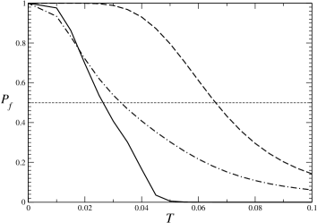
Figure 1: Folding probability $P_{f}$ estimated from Eq.(12) as a function of temperature $T$. The full, dot–dashed and dashed lines correspond to S0, S2 and S1, respectively.

	MD	graph
S0	0.044	0.026
S1	0.061	0.066
S2	0.044	0.033

Table 3: folding temperatures as computed by means of MD simulations (table 1) and of the analytical expression of the stationary distribution on the connectivity graph.

These results confirm that equilibrium properties of the directed graph are quantitatively consistent with MD predictions.

The comparison between MD and the graph dynamics (GD) concerns dynamical indicators. We report hereafter the results of numerical simulations for the average exit time from a region in the landscape and for the first passage time from the native state. The former aims at verifying the conjecture that MD corresponds to a sequence of thermally activated transitions through the nodes of the directed graph; the latter amounts to obtain a quantitative estimate of the time scale involved in the folding process.

GD is performed by assigning the average time spent at node $i$ as follows :

$$\langle t_{i}\rangle={1\over\sum_{k}\Gamma_{i,k}}.$$ (16)

The index $k$ runs over all the nodes directly connected with $i$. The probability of moving from node $i$ to node $j$ is given by the expression

$$\Pi_{i,j}=\Gamma_{i,j}\langle t_{i}\rangle$$ (17)

Accordingly, a trajectory on the directed graph can be represented by an ordered set of symbols $(i,j,k,\cdots,m,n)$ labeling the sequence of visited nodes: its time duration is given by the expression

$$t=\sum_{\alpha=i}^{n}\langle t_{\alpha}\rangle\,\,\,.$$ (18)

Notice that the time scale which establishes the correspondence between MD and GD is the inverse of the dissipation rate $\gamma$ (see Section II.2 and eq.(7)) .

In Table 4 we report for two temperatures, $T=T_{g}=0.4$ and $T=T_{f}=0.6$, the average exit time for sequence S1 from the native minimum, from the first shell (i.e., the set of the 66 minima directly connected with the native one) and from the set of minima ${\mathcal{M}}$, whose angular distance $d_{\theta}$ from the native state is smaller than 0.4. The latter set contains 2341 minima, including the first shell.

MD averages have been performed over $10^{3}$ trajectories starting from each minimum in the considered set, while GD averaged have been performed over $10^{4}$ stochastic paths. The data exhibits a reasonable agreement, if one considers that Langer’s formula is known to systematically overestimate the actual transition rates $\Gamma_{i,j}$ hanggi  .

Measurements of the first passage time of S1 through its native minimum have also been performed by averaging over $10^{3}$ MD trajectories and over $10^{4}$ GD paths. We have considered three different classes of initial conditions: the minima in the first shell, the set ${\mathcal{M}}$, and the larger set of minima ${\mathcal{N}}$, whose potential energy is smaller than $V(0)+1/2K_{B}T_{f}L^{\prime}=-3.45$ ( 17726 minima). For $T=0.04$ we find a good quantitative agreement between MD and GD (see Table 5), while for $T=0.06$ the first passage time on the the graph is much smaller then the MD predictions. Apart the approximation due to the Langer’s estimate of the transition rate, the main reason for this discrepancy has to be attributed to the poor reconstruction of the energy landscape for high values of the potential energy. In fact, we have checked that by considering the subset of trajectories which go to the native minimum without escaping from the set of initial minima, average first passage times converge to much closer values. This implies that MD visits regions of the energy landscape that are scarcely accessible to the graph dynamics. Only for temperatures smaller than $T_{f}$ this effect is highly reduced and MD trajectories tend to remain confined in a smaller portion of the energy landscape, which is more accurately represented in the graph. We want to point out that a finer sampling of the energy landscape would demand a sensible computational effort even for producing a small improvement.

Performing similar kinds of measurements for S0 and S2 at $T=0.04$ is practically unfeasible for MD simulations, since the average exit and folding times increase at least of two orders of magnitude with respect to S1. Measurements of the average folding time at $T=0.06$ starting from the set of minima with potential energy below $1/2K_{B}T_{f}L^{\prime}$ give $1.3\times 10^{6}$ for MD and $9.8\times 10^{5}$ for GD. Since the quantitative agreement is maintained we can reasonably conjecture that it should hold also at lower temperatures. Accordingly, we have estimated by GD the average first passage time of S0 and S2 at $T=0.04$. In both cases we have found values three orders of magnitude larger than those obtained for S1. We can conclude that, at variance with MD, the graph dynamics allows to estimate the average folding time even for $T<T_{f}$, thus providing a clear characterization of a fast folder with respect to generic polymers.

From the native state
	T=0.04	T=0.06
MD	4193	164
GD	3509	85
From the 1st shell
	T=0.04	T=0.06
MD	23459	446
GD	13077	243
From the set ${\mathcal{M}}$
	T=0.04	T=0.06
MD	326855	2052
GD	107775	704

Table 4: Comparison of average escape times of S1 from three different sets of initial conditions computed by MD and GD simulations at temperatures $T=0.04$ and $T=0.06$. The first shell contains 66 minima, while the set ${\mathcal{M}}$ contains 2341 minima.

From the 1st shell
	T=0.04	T=0.06
MD	5746	1153
GD	4307	461
From the set ${\mathcal{M}}$
	T=0.04	T=0.06
MD	8535	4120
GD	4434	512
From the set ${\mathcal{N}}$
	T=0.04	T=0.06
MD	6947	5759
GD	4566	583

Table 5: Comparison of average first passage times at the native state from three different sets of initial conditions computed by MD and GD simulations at temperatures $T=0.04$ and $T=0.06$. The first shell contains 66 minima, the set ${\mathcal{M}}$ contains 2341 minima and the set ${\mathcal{N}}$ contains 17726 minima .

IV Renormalization of the directed graph

As we have shown in the previous section MD and GD exhibit a reasonable quantitative agreement, while numerical simulations of the latter are faster than the former. On the other hand, a considerable computational price has been payed for obtaining a suitable reconstruction of the energy landscape. The very advantage of the directed graph representation stems from the possibility of applying an effective renormalization procedure. In fact, at a given temperature $T$ the directed graph can be renormalized by eliminating all those links (saddles) corresponding to energy barriers smaller than $K_{B}T$. In practice, the procedure can be performed by reducing the pair of nodes connected by such a barrier to a single node, whose connectivity is renormalized accordingly. More precisely, the renormalization algorithm goes through the following steps.

• For any pair of connected nodes $i$ and $j$ we compute

  $$\Delta V_{i,j}=V(s_{i,j})-V(j)$$ (19)

  if $V(j)>V(i)$;

• the $\Delta V_{i,j}$ are listed in increasing order and we choose the subset

  $$\Sigma=\{\Delta V_{i,j}:\Delta V_{i,j}\leq K_{B}T\}\,\,\,;$$ (20)

• starting from the smallest element of $\Sigma$ the graph is renormalized by first assimilating node $j$ with node $i$: the renormalized equilibrium eigenvector ${\tilde{w}}^{(1)}$ and the renormalized rates $\tilde{\Gamma}_{k,j}$ are defined as follows:

  $$\tilde{w}^{(1)}_{i}=w^{(1)}_{i}+w^{(1)}_{j}$$ (21)

  $$\tilde{\Gamma}_{k,i}=\begin{cases}\Gamma_{k,j}\,\,\,\text{if}\,\,\,\Gamma_{k,j}=0\\ \Gamma_{k,i}+\Gamma_{k,j}\,\,\,\text{otherwise}\end{cases}$$ (22)

  and

  $$\tilde{\Gamma}_{i,k}=\begin{cases}\frac{\Gamma_{j,k}w^{(1)}_{j}}{w^{(1)}_{j}+w^{(1)}_{i}}\,\,\,\text{if}\,\,\,\Gamma_{k,i}=0\\ \frac{\Gamma_{j,k}w^{(1)}_{j}+\Gamma_{i,k}w^{(1)}_{i}}{w^{(1)}_{j}+w^{(1)}_{i}}\,\,\,\text{otherwise}\end{cases}$$ (23)

• then we pass to the second lowest value in the set $\Sigma$ and proceed sequentially until all the elements of this set are renormalized.

The renormalized rates $\tilde{\Gamma}_{i,j}$ define a renormalized evolution matrix $\tilde{W}$, whose equilibrium eigenvector is $\tilde{w}^{(1)}$. It can be easily argued that detailed balance conditions (13) are maintained for the renormalized quantities. Moreover, since it only involves node removal, the procedure just outlined maintains the original ordering of the graph nodes.

The renormalization procedure transforms also the discrete connectivity matrix $\Gamma_{\mathrm{d}}$ and the discrete Laplacian matrix $W_{\mathrm{d}}$ to $\tilde{\Gamma}_{\mathrm{d}}$ and $\tilde{W}_{\mathrm{d}}$, respectively. In the following section we shall first discuss how the topological properties of the renormalized directed graph depend on temperature. Afterwards, the corresponding dynamical features will be analyzed.

IV.1 Topological properties of the renormalized connectivity graph

The renormalization procedure presented in Section IV depends on the temperature and here we want to analyze how it can change the topological properties of the directed graph.

In Fig. (2) we show how the number of nodes $N$ and the number of connections per node ${\bar{\sigma}}=S/N$ change with the temperature, for the three sequences defined in Section II. Temperatures are varied in the range $0\leq T\leq 0.08$, thus encompassing both the glassy and the folding temperatures of all sequences (see Table I). The homopolymer S0 exhibits a very slow exponential decay of $N$, while $\sigma$ slightly increases. Conversely, for S1 and S2, $N$ reduces by more than one order of magnitude, while $\sigma$ uniformly decreases beyond $T=0.02\,$. These results stress the topological differences between the graph representations of the homopolymer S0 and of the heteropolymers S1 and S2. In the explored range of temperatures the graph of S0 is poorly affected by renormalization. This is due to the peculiar structure of its energy landscape: most barrier heights separating local minima from their neighbors are deep enough to keep their role of ”hubs” in the renormalized graph, while a relatively small fraction of minima are absorbed by the hubs, thus slightly increasing the average connectivity.

In the graph representation of S1 and S2 the number of hubs is significantly reduced, because an increasing number of barrier heights is renormalized as temperature increases. Moreover, apart an initial increase up to 7, $\sigma$ drops to much smaller values. The main reason for this sensible reduction of the average connectivity is essentially due to the fact that most of the hubs share with the renormalized nodes connections with the same set of neighboring nodes, at variance with S0, where the connectivity is much more sparse. A simple argument accounts for these opposite mechanisms. Let us suppose that node $j$, with connectivity $s_{j}$, is renormalized to node $i$, with connectivity $s_{i}$. The connectivity of the hub $i$ becomes equal to ${\tilde{s}_{i}}=s_{i}+s_{j}-c-2$ if $c$ is the number of connections with neighboring nodes common to $i$ and $j$. There are two extreme situations: if $c=0$ (no common connections) then ${\tilde{s}}_{i}=s_{i}+s_{j}-2$, while if $c=s_{i}-1=s_{j}-1$ ($i$ and $j$ have the same neighbors) then ${\tilde{s}_{i}}=s_{i}-1$. This argument indicates that above $T=0.02$ many nodes in the graphs of S1 and S2 are highly connected among themselves so that renormalization acts as an overall reduction of the average connectivity. More precisely, only fewer and fewer hubs maintain a high connectivity, while the great majority assumes the role of peripheral nodes. This picture is also confirmed by looking at the distribution of the renormalized average connectivity $\sigma$ at different temperatures: it is practically unmodified for S0, while for S1 and S2 it tends to be sharply peaked at 1 as $T$ increases. In Fig.s (3) , (4) and (5) we report the fraction of nodes with connectivity $\sigma$, $\nu(\sigma)=N(\sigma)/N$, versus $\sigma$ for different values of $T$. Notice that both $N(\sigma)$ and $N$ vary with the renormalization temperature .

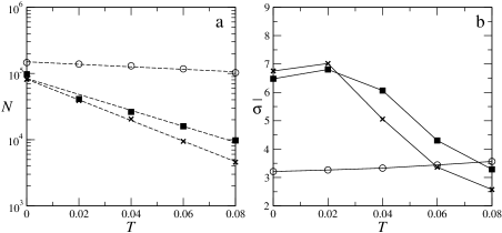
Figure 2: Number of nodes $N$ (a) and average connectivity $\bar{\sigma}$ (b) of the renormalized graph versus temperature $T$ for S0 (empty circles), S1 (crosses) and S2 (filled squares). In (a) the dashed lines are exponential fits of the data, due to the adopted log-lin representation. The full lines in (b) are drawn to guide the eyes.

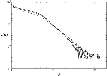
Figure 3: Sequence S0: the fraction of nodes with connectivity $\sigma$, $\nu(\sigma)$, in log-log scale at $T=0$ (full line), $T=0.04$ (dashed line) and $T=0.08$ (dot-dashed line).

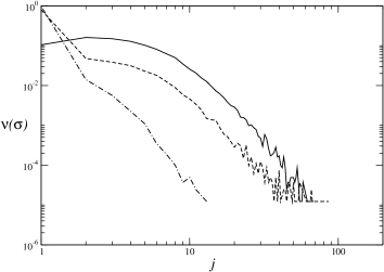
Figure 4: Sequence S1: the fraction of nodes with connectivity $\sigma$, $\nu(\sigma)$, in log-log scale at $T=0$ (full line), $T=0.04$ (dashed line) and $T=0.08$ (dot-dashed line).

Figure 5: Sequence S2: the fraction of nodes with connectivity $\sigma$, $\nu(\sigma)$, in log-log scale at $T=0$ (full line), $T=0.04$ (dashed line) and $T=0.08$ (dot-dashed line).

A special role in the renormalization procedure is played by the ”native” node, which becomes the main hub of the network, since it collects an increasing number of renormalized nodes as $T$ increases. This effect is significantly more pronounced for S1 and S2 with respect to S0: for instance, at $T=0.08$ $\sigma_{0}\sim 10^{4}$ for S1 and S2, while $\sigma_{0}\sim 10^{3}$ for S0 .

The topological properties of the directed graphs considered in this section can be also described by determining their spectral dimension $\tilde{d}$ burioni . In an infinite graph this quantity is defined by the formula

$$R(\omega)\sim\omega^{\tilde{d}}$$ (24)

where $R(\omega)$ is the integrated density of harmonic vibrational modes with frequency $\omega$. It is worth recalling that in our model we are dealing with the spectrum of the discrete Laplacian matrix $W_{\mathrm{d}}$, with finite rank $N$ (see Section II.3) . If we denote its eigenvalues with $\lambda_{1}<\lambda_{2}<\cdots<\lambda_{\mathrm{k}}<\cdots<\lambda_{\mathrm{N}}$ we can define the integrated density of eigenvalues $R(\lambda_{\mathrm{k}})$. In this case, we can reasonably assume that, if the rank $N$ of $W_{\mathrm{d}}$ is sufficiently large, by identifying $\omega$ with $\omega_{k}=\lambda_{k}^{1/2}$ the spectral dimension can be estimated through the approximate relation

$$R(\lambda_{k})\sim\lambda_{k}^{\tilde{d}/2}$$ (25)

In Fig. 6 we show that one obtains close estimates of the spectral dimension ($\tilde{d}\approx 6.5$) for the connectivity graphs of all the three sequences considered in this paper. In an infinite graph the application of the renormalization procedure described in Section IV cannot change the value of $\tilde{d}$ burioni . This is what happens also for the finite graph representing the homopolymer S0: Fig. 7 shows that, independently of the temperature $T$, the value of $\tilde{d}$ in the renormalized graph is constant. Conversely, for the heteropolymers S1 and S2 the value of $\tilde{d}$ decreases to a value close to 5 for $T>0.02$ (see Fig. 8, where we report the data for sequence S1, which exhibits the same behavior of sequence for S2). This indicates that, beyond this temperature, the renormalization procedure modifies the topological properties of the finite directed graphs: regions of high connectivity collapse into big hubs, while in the renormalized graph the average connectivity is significantly reduced. This is consistent with what is shown in Fig. 2 .

We can conclude that all topological indicators analyzed in this section allow to distinguish between the homopolymer S0 and the other heteropolymers. On the other hand, no significant difference between S1 and S2 can be identified. As we have discussed in Section III this seems to emerge only by considering dynamical properties of the directed graphs. In particular, in what follows we are going to show that this different dynamical features are maintained also in the renormalized graphs.

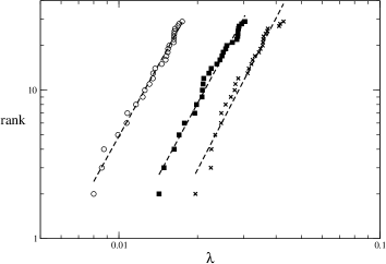
Figure 6: Log–log plot of the spectrum of eigenvalues of the discrete Laplacian matrix $W_{\mathrm{d}}$ of the zero–temperature connectivity graph of S0 (empty circles), S1 (crosses) and S2 (filled squares). The dashed line refer to power–law with exponents 3.3  .

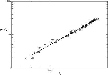
Figure 7: Log–log plot of the spectrum of eigenvalues of the discrete Laplacian matrix $W_{\mathrm{d}}$ of S0 for five different temperatures: $T=0.00,0.02,0.04,0.06,0.08$. We have used the same symbols independently of temperature to point out that data collapse on the same curve: the full line corresponds to the power-law fit with exponent 3.1. .

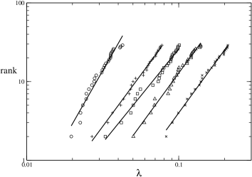
Figure 8: Log–log plot of the spectrum of eigenvalues of the discrete Laplacian matrix $W_{\mathrm{d}}$ of S1 for five different temperatures: $T$=0.00 ($\circ$), 0.02 (+), 0.04 ($\Box$), 0.06 ($\triangle$), 0.08 ($\times$). The data obtained for different temperatures are shifted horizontally by an arbitrary constant factor in order to obtain a better view. Notice that the power-law fit passes from its maximum value, 3.4 at $T=0$ to a minimum value of 2.5  above $T=0.02$.

IV.2 Relaxation times and the low frequency spectrum of the Laplacian matrix

One can easily realize that obtaining a complete characterization of the spectrum of the Laplacian matrix $W$ defined in (10) demands the diagonalization of a matrix whose rank is ${\cal O}(10^{5})$ (see Table 2). This is practically unfeasible. On the other hand, we are at least interested in reconstructing the part of the spectrum of $W$ containing the smallest eigenvalues $r_{k}$, $k=2,3,\cdots$, which are related to the largest equilibration time scales. This task can be accomplished by using Lanczos-like algorithms of the ARPACK Library arpack .

We have first checked that the lowest part of the spectrum of $W$ and of its renormalized version $\tilde{W}$ are consistent. In fact, since the renormalization procedure described in the previous section amounts to a series of local transformations on the directed graph, we expect that the first nonzero eigenvalues should not vary. The corresponding eigenvectors, $w^{(k)}$, $k=2,3,\cdots$ should as well keep their ”structure”, modulo the renormalization procedure, which changes their dimension (see Section IV) . Such a comparison has been performed for the directed graph of S1 at $T=0.08$ . Table 6 reports the rank of $\tilde{W}$ at various temperatures for the three sequences investigated.

T	S0	S1	S2
0.02	138791	41139	38997
0.04	130326	20537	26292
0.06	117328	9430	15943
0.08	102933	4576	9736

Table 6: Rank of the renormalized Laplacian matrix $\tilde{W}$ the three investigated sequences at various temperatures below $T_{\theta}$.

Relying upon this analysis, we can assume that the interesting spectral properties of $W$ can be extracted from $\tilde{W}$ (by exploiting also the symmetrization procedure described in Section II.3). In fact, if we consider lower values of the temperature, i.e. $T=0.06$ and $T=0.04$, the rank of $\tilde{W}$ reduces for S1 to 9430 and 4576, respectively (see Table 6). On the other hand, a direct comparison with the spectrum of $W$ would demand a too high computational cost: at lower temperatures the relative separation between the eigenvalues at the lower end of the spectrum quickly approaches machine precision thus dramatically slowing down the convergence rate of the diagonalization algorithm arpack .

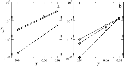
Figure 9: The eigenvalues $r_{k}$, for $k=2,3,4$ S1 versus temperature $T$ in log–reciprocal scale for S1 (a) and S2 (b) . The dashed lines are exponential fits to the data.

In Fig.(9) we show the dependence of the smallest non-zero eigenvalues of $\tilde{W}$ on the temperature $T$ for sequences S1 and S2 . In both cases we obtain evidence of an Arrhenius–like behavior

$$r_{k}\simeq A\exp{(-B/K_{B}T)}.$$ (26)

where $A$ and $B$ are suitable constants, which depend on the sequence and on $k$.

The corresponding eigenvectors are shown in Fig.s (10) and (11). To ease reading we report the absolute value of the components of eigenvectors $w^{(2)}$, $w^{(3)}$ and $w^{(4)}$, since, as shown in Appendix A, their components sum to 0 and therefore fluctuate wildly between positive and negative values. The eigenvectors $w^{(1)}$ is also reported for comparison. We recall that the eigenvector components are ordered according to the energy of the corresponding graph node. All the eigenvectors of S2 are localized on some node of the graph, as well as the $w^{(2)}$ eigenvector of S1. The other eigenvectors of S1 are instead delocalized.

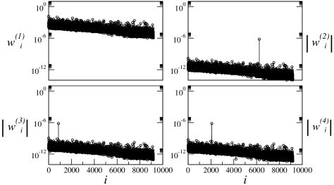
Figure 10: Components of $w^{(1)}$ and absolute value of the components of $w^{(2)}$, $w^{(3)}$ and $w^{(4)}$ for the slow–folder S2 at $T=0.06$.

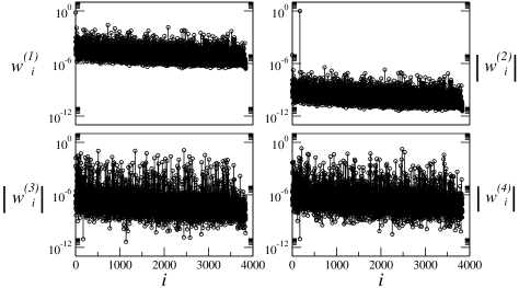
Figure 11: Components of $w^{(1)}$ and absolute value of the components of $w^{(2)}$, $w^{(3)}$ and $w^{(4)}$ for the fast–folder S1 at $T=0.04$.

We have verified that, for the localized eigenvectors, the energy $B$ amounts to the height of the lowest energy barrier separating the localized node from the graph. Nonetheless this energy barrier is quite high and, in this sense, the node can be viewed as a kinetic trap of GD. We have also found that most of the first 50 non–zero eigenvectors of S2 are localized as those shown in Fig. (10). Accordingly, this suggest that a great deal of nodes play the role of a kinetic trap, thus slowing-down any dynamical process on the graph.

For what concerns the delocalized eigenvectors of S1, $B$ can be interpreted as an effective energy barrier separating different subsets of nodes in the graph. This interpretation can be supported by the following argument. Let us suppose that a graph is subdivided into two subgraphs $\mathcal{A}$ and $\mathcal{B}$, weakly connected between themselves. By dividing each component $w^{(2)}_{i}$ by $w^{(1)}_{i}$ one obtains a ”normalized” eigenvector $\bar{w}^{(2)}$, whose components are split into two sets of values (see Appendix B for details) , which identify the nodes contained into the two subgraphs. The normalized eigenvectors $\bar{w^{(3)}}$ and $\bar{w^{(4)}}$, shown in the upper panels of Fig.(12), exhibit a similar scenario, although they are split into more than two sets of values. This indicates that the graph structure of S1 is more intricated than in the example discussed in Appendix B. Nonetheless, the interpretation of $B$ as an effective barrier height separating different regions of the graph remains valid. Notice that the corresponding eigenvalues $r^{3}$ and $r^{4}$ are more than four orders of magnitude larger than $r^{2}$. This shows that the perturbative argument presented in the Appendix provides only a qualitative approximation of what seen in Fig.(12).

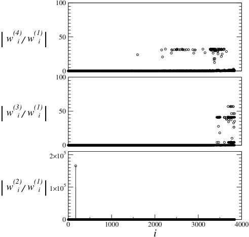
Figure 12: Absolute value of the components of the normalized eigenvectors $\bar{w^{(2)}}$, $\bar{w^{(3)}}$ and $\bar{w^{(4)}}$ for the fast–folder S1 at $T=0.04$.

For what concerns the folding process, we have already observed in Section III that the time scales of equilibration are orders of magnitude larger than those characterizing the first passage time through the native valley (i.e. the native minimum and the connected minima). In fact, according to our definition of the folding temperature, we can guess that over the equilibration time scale approximately $50\%$ of the time is spent in the native valley, despite it contains a very small fraction of the minima (nodes) in the landscape (directed graph). In the renormalized representation of the directed graph we expect that the quantitative determination of the average first passage time through the native valley (that is reduced to a single node, as a result of the renormalization of the minima connected to the native one) is preserved, provided the graph is renormalized for temperatures $T\leq T_{f}$. For instance, we have verified that this is the case for S1 at $T=0.04$ where the folding time on the renormalized graph amounts to 1892 when averaged over $10^{4}$ paths.

V Conclusions and Perspectives

Many phenomena of biological interest are associated with equilibrium and non–equilibrium processes in polypeptidic chains. A suitable description and understanding of such processes is far from trivial in these complex structures. This is the main reason why in this manuscript we have decided to consider a sufficiently simple and widely investigated model Still for testing an effective approach to these problems. In particular, we have analyzed two heteropolymers and one homopolymer in order to point out differences and analogies among various typical polypeptidic sequences. In fact, one of the heteropolymer is known to behave as a ”fast folder”, at variance with the other ones, which exhibit a much slower relaxation dynamics to their native states.

As a first step we have described a strategy for reconstructing the energy landscape of these simple chains. The search for minima and first order saddles is performed by combining different algorithms aiming at a sufficiently careful reconstruction of the landscape close to the native minimum, up to values of the energy of the order of $K_{B}T_{f}$, where $T_{f}$ denotes the folding temperature. Since the number of minima and saddles increases with the energy, the computational cost is already quite high up to $K_{B}T_{f}$: going beyond this value is practically unfeasible. On the other hand, performing a more extended search is not expected to add relevant information. In fact, we have checked that the main dynamical mechanisms associated with the folding process and with the relaxation to equilibrium are very well reproduced, even if most of the stationary points in the energy landscape above $K_{B}T_{f}$ are discarded.

The following step amounts to exploit our knowledge of the relevant part of the energy landscape for reconstructing a directed graph representation of the dynamics. Actually, the temperature dependent molecular dynamics performed in the energy landscape can be replaced by a Markov-chain dynamics on a directed graph. The nodes of the graph correspond to the local minima of the energy landscape, while the first order saddles connecting such minima are represented by the links of the graph. The strength of the links is measured by the Langer’s estimate hanggi of the hopping rates between connected minima. The directed nature of the graph is associated with the asymmetry due to the different energies of the two connected minima. We have shown that, for temperatures close or below $T_{f}$, MD simulations are essentially in good quantitative agreement with GD. Anyway, in general the latter systematically underestimate the former, mainly because it has not access to the poorly reconstructed portion of the energy landscape above $K_{B}T_{f}$.

The main advantage of using a graph representation is that one can apply a renormalization procedure, which keeps the topological as well as the dynamical features of the model, while significantly reducing the dimensionality of the graph as temperature is increased. Actually, the procedure described in Section IV allows to aggregate many of the original nodes into renormalized ”hubs”, characterized by a high connectivity, while a great deal of nodes exhibits a weak connectivity. This effect is much more relevant in the heteropolymers, than in the homopolymer, thus indicating that the topological properties are quite different in the two cases. Anyway, this allows us to conclude that the homopolymer, thanks to its spatially homogeneous structure, exhibits peculiar topological properties with respect to any disordered sequence of peptides. This notwithstanding, in the simple model considered in this paper we have evidence that topological properties are not sufficient for discriminating between a ”fast” and a ”slow” folder, which are known to correspond to sequences S1 and S2, respectively. This does not exclude that topological indicators should not be effective in more realistic models of proteins. Nonetheless, we can affirm that dynamical properties analyzed in the MD, GD and renormalized GD provide a clear identification of the ”fast folder” and are expected to be effective for the wide class of models of polypeptides considered in the literature. In particular, we find that the average first passage time from the native configuration, which provides an estimate of the folding time, is at least two orders of magnitude smaller for the ”fast folder” S1 than for the other sequences. By comparing this time scale with the typical equilibration time scale associated with the inverse of the smallest eigenvalue of the Laplacian matrix of the renormalized graph we find that they are comparable for S0 and S2, while for S1 it is three orders of magnitude smaller. Considering that for S1 at $T_{f}$ more than $50\%$ of the equilibrium measure is concentrated in the native valley, we can conclude that the dynamics of the fast folder spends a great deal of time exploring configurations close to its native state, even during the transient to equilibration. This points out that the folding process can be viewed as a genuine nonequilibrium process, since the equilibration time scales are too large to be compared with experimental estimates of the typical folding time of a polypeptidic chain.

We want to conclude by pointing out that the methods described in this paper can be applied also to more realistic models of polypeptides and single–domain proteins. It is evident that the reconstruction of the relevant portion of the energy landscape associated with the folding and equilibration processes may yield high computational costs. Nonetheless, the renormalization procedure can provide an effective representation of the kinetics of these models, up to the time scales typical of the equilibration process, which usually cannot be explored by the traditional MD approaches.

Appendix A Properties of the Master Equation

We now show some useful properties of the Master equation and of the eigenvectors of the Laplacian matrix.

As a preliminary observation we note that, by summing both sides of the Master equation over all the nodes of the graph and invoking the detailed balance condition, one can easily verify that the total probability is conserved:

$${d(\sum_{i}P_{i})\over dt}=-\sum_{i,j=1}^{N}P_{i}\Gamma_{i\rightarrow j}+\sum_{i,j}P_{j}\Gamma_{j\rightarrow i}=0.$$ (27)

The normalization condition $\sum_{i}P_{i}(t)=1$ therefore holds at every $t$, which, as we will see later, induces some constraints on the projections of realistic probability vectors on the eigenvectors of the Laplacian Matrix $W$.

As already mentioned, $W$ can be cast into a symmetric form trough a similarity transformation. It therefore admits a complete basis of orthogonal eigenvectors, each describing a different mode of decay to equilibrium. Besides orthogonality, the eigenvectors of $W$ share the additional property that their components are zero-sum. In fact, from the eigenvalue equation $Ww^{(j)}_{i}=\lambda^{(j)}w^{(j)}_{i}$ one gets

$$w^{(j)}_{i}={-\sum_{k=1}^{N}w^{(j)}_{i}\Gamma_{i,k}+\sum_{k=1}^{N}w^{(j)}_{k}\Gamma_{k,i}\over\lambda^{(j)}}.$$ (28)

Summing over $i$ each members and once again invoking detailed balance, leads to

$$\sum_{i=1}^{N}w^{(j)}_{i}=0.$$ (29)

The only eigenvector that defies this demonstration is $w^{(1)}$ the null eigenvector defined in Equation (12), which actually has positive components and can be normalized to unity. Using this normalization one can write:

$$\sum_{i=1}^{N}w^{(j)}_{i}=\delta_{1,j}.$$ (30)

Actually the fact that eigenvector have zero sum is just a consequence of the fact that the master equation conserves probability. Indeed, since eigenvectors form a complete basis, each probability distribution of initial conditions on the graph $P(0)$ can be expressed as $P(0)=\sum_{j=1}^{N}\alpha_{j}w^{(j)}$. It will then evolve in time according to

$$P(t)=\sum_{j=1}^{N}\alpha_{j}w^{(j)}\exp^{-r_{j}t}.$$ (31)

Summing over the components of $P(t)$

$$\sum_{i=1}^{N}P_{i}(t)=\sum_{j=1}^{N}\alpha_{j}\;\delta_{1,j}\exp^{-r_{j}t}=\alpha_{0}.$$ (32)

Hence, in order to have $\sum_{i=1}^{N}P_{i}(t)=1$, $\alpha_{1}$ must necessarily be 1.

Appendix B Spectral clustering

We now justify the use of reweighted components as an effective tool to uncover the inherent structure of eigenvectors. We define reweighted components of a vector $v$ on a graph as the ratio site–to–site of the vector component to the local value of the stationary probability: $\bar{v_{i}}=v_{i}/w_{i}^{(0)}$. We will here extend an argument originally proposed for discrete graphs ding to weighted ones and show that, when a graph is divided into two weakly connected subgraphs $\mathcal{A}$ and $\mathcal{B}$, the reweighted components of the first nonzero eigenvector assume only two possible values one for $\mathcal{A}$ and one for $\mathcal{B}$.

The Laplacian Matrix $W$ can be written as the sum of two matrices: $W=D-\Gamma^{T}$, where $\Gamma$ is the transition rate matrix and $D$ a diagonal matrix $D_{i,j}=\delta_{i,j}\sum_{k=1}^{N}\Gamma_{i,k}$.

First of all, we consider the case in which the graph is composed of two disconnected subsets of nodes $\mathcal{A}$ and $\mathcal{B}$. In this case the Laplacian matrix will be referred to as $W^{0}$. Since $\Gamma_{i,j}=0$ for each $i\in\mathcal{A}$ and $j\in\mathcal{B}$, $W^{0}$ can be written as

$$W^{0}=\left(\begin{array}[]{cc}D_{\mathcal{AA}}-\Gamma_{\mathcal{AA}}^{T}&0\\ 0&D_{\mathcal{BB}}-\Gamma_{\mathcal{BB}}^{T}\end{array}\right)$$ (33)

Let now use the null eigenvector $w^{(1)}$ of $W^{0}$ to construct two vectors $w^{\mathcal{A}}$ e $w^{\mathcal{B}}$ as follows:

$$w_{i}^{\mathcal{A}}=\left\{\begin{array}[]{lc}w_{i}^{(1)}&i\in\mathcal{A}\\ 0&i\in\mathcal{B}\end{array}\right.,\;\;w_{i}^{\mathcal{B}}=\left\{\begin{array}[]{lc}0&i\in\mathcal{A}\\ w_{i}^{(1)}&i\in\mathcal{B}\end{array}\right.$$ (34)

It is easy to show that both $w^{\mathcal{A}}$ and $w^{\mathcal{B}}$ are eigenvectors of $W^{0}$ with a null eigenvector, and the same holds for any linear combination $v=aw^{\mathcal{A}}+bw^{\mathcal{B}}$. More generally when a graph is composed of $n$ disconnected subgraphs the kernel of its Laplacian matrix is has dimension $n$.

Let’s now suppose that the two subgraphs $\mathcal{A}$ and $\mathcal{B}$ are not properly disconnected but do share a small number of connections. In this case the Laplacian matrix has the form $W=W^{0}+W^{1}$, with

$$W^{1}=\left(\begin{array}[]{cc}D_{\mathcal{AB}}&-\Gamma_{\mathcal{AB}}^{T}\\ -\Gamma_{\mathcal{BA}}^{T}&D_{\mathcal{BA}}\end{array}\right).$$ (35)

where $\Gamma_{\mathcal{AB}}$ and $\Gamma_{\mathcal{BA}}$ carry the information about connections between $\mathcal{A}$ and $B$, while $D_{\mathcal{AB}}$ and $D_{\mathcal{BA}}$ carry the information on the effect these connections have on the diagonal of the Laplacian matrix.

We now look for the eigenvectors of $W$ among vectors of the form $v=aw^{\mathcal{A}}+bw^{\mathcal{B}}$:

$$Wv=(W^{0}+W^{1})(aw^{\mathcal{A}}+bw^{\mathcal{B}})=$$

$$=W^{1}(aw^{\mathcal{A}}+bw^{\mathcal{B}}).$$ (36)

In other words if any eigenvector of $W$ exists that is a linear combination of $w^{\mathcal{A}}$ and $w^{\mathcal{B}}$ it is also an eigenvector of $W^{1}$. We will therefore look for the eigenvectors of this last matrix having the desired form $aw^{\mathcal{A}}+bw^{\mathcal{B}}$.

For sufficiently small $W^{1}$ the vector $W^{1}(aw^{\mathcal{A}}+bw^{\mathcal{B}})$ can be approximately written as a linear combination of $w^{\mathcal{A}}$ and $w^{\mathcal{B}}$. To this purpose we introduce the projector on the space of the linear combinations of $w^{\mathcal{A}}$ and $w^{\mathcal{B}}$

$$\Pi_{\mathcal{A}\mathcal{B}}=(w^{\mathcal{A}},w^{\mathcal{B}})$$ (37)

where $(w^{\mathcal{A}},w^{\mathcal{B}})$ is a $N\times 2$ matrix whose columns are the two column vectors $w^{\mathcal{A}}$ and $w^{\mathcal{B}}$. The vector $W^{1}(aw^{\mathcal{A}}+bw^{\mathcal{B}})$ can now be written as:

$$W^{1}(aw^{\mathcal{A}}+bw^{\mathcal{B}})\simeq\Pi_{\mathcal{AB}}W^{1}(aw^{\mathcal{A}}+bw^{\mathcal{B}})=$$

$$=\tilde{W^{1}}\left(\begin{array}[]{c}a\\ b\end{array}\right)(w^{\mathcal{A}},w^{\mathcal{B}})$$ (38)

where we have introduced $\tilde{W^{1}}=\Pi_{\mathcal{AB}}^{T}W^{1}\Pi_{\mathcal{AB}}$, a $2\times 2$ matrix that reproduces the effect of $W^{1}$ in the subspace of the linear combinations of $w^{\mathcal{A}}$ and $w^{\mathcal{B}}$. After some algebra $\tilde{W^{1}}$ reads

$$\tilde{W^{1}}={\small\left(\begin{array}[]{cc}\sum_{i\in\mathcal{A},j\in\mathcal{B}}{w^{(1)}_{i}}^{2}\Gamma_{i,j}&-\sum_{i\in\mathcal{A},j\in\mathcal{B}}w^{(1)}_{i}w^{(1)}_{j}\Gamma_{j,i}\\ +\sum_{i\in\mathcal{B},j\in\mathcal{A}}w^{(1)}_{i}w^{(1)}_{j}\Gamma_{j,i}&\sum_{i\in\mathcal{B},j\in\mathcal{A}}{w^{(1)}_{i}}^{2}\Gamma_{i,j}\end{array}\right)}.$$ (39)

Since $w^{(1)}$ satisfies the detailed balance, and existing a connection from $\mathcal{B}$ to $\mathcal{A}$ for each connection from $\mathcal{A}$ to $\mathcal{B}$, one has:

$$\sum_{j\in\mathcal{B}}w^{(1)}_{i}\Gamma_{i,j}=\sum_{j\in\mathcal{B}}w^{(1)}_{j}\Gamma_{j,i}\;\;\;\;\;\;\forall i\in\mathcal{A}.$$ (40)

Analogously:

$$\sum_{j\in\mathcal{A}}w^{(1)}_{i}\Gamma_{i,j}=\sum_{j\in\mathcal{A}}w^{(1)}_{j}\Gamma_{j,i},\;\;\;\;\;\;\forall i\in\mathcal{B}.$$ (41)

We can therefore define two quantities $\alpha=\sum_{i\in\mathcal{A},j\in\mathcal{B}}w^{(1)}_{i}w^{(1)}_{j}\Gamma_{j,i}$ and $\beta=\sum_{i\in\mathcal{B},j\in\mathcal{A}}w^{(1)}_{i}w^{(1)}_{j}\Gamma_{j,i}$ which cast $\tilde{W^{1}}$ in a particularly simple form

$$\tilde{W^{1}}=\left(\begin{array}[]{cc}\alpha&-\alpha\\ -\beta&\beta\end{array}\right)$$ (42)

It is important to notice that, if the two subgraphs $\mathcal{A}$ are weekly connected $\alpha$ and $\beta$ will be relatively small, since there are few connections such that $\Gamma_{j,i}>0$ for $i\in\mathcal{A}$ and $j\in\mathcal{B}$.

The two eigenvalues of $\tilde{W^{1}}$ are 0 and $\alpha+\beta$, referring respectively to the eigenvectors

$$\left(\begin{array}[]{c}1\\ 1\end{array}\right)\;\;\;\;\;\mathrm{and}\;\;\;\;\;\left(\begin{array}[]{c}\alpha\\ -\beta\end{array}\right).$$ (43)

It can finally be shown that backprojecting with $\Pi_{\mathcal{AB}}^{T}$ this two eigenvectors of $\tilde{W^{1}}$ to the entire $N$-dimensional space one obtains two eigenvectors of $W^{1}$ characterized by the same eigenvalues. According to Equation 36 these are also eigenvectors of $W$. More precisely by this procedure one obtains

• $w^{\mathcal{A}}+w^{\mathcal{B}}$ which obviously coincides with $w^{(1)}$ and is associated to the null eigenvalue also according to the perturbative calculation

• $u=\alpha w^{\mathcal{A}}-\beta w^{\mathcal{B}}$, associated to the eigenvalue $\alpha+\beta$ which is a small number and will therefore lay in the low end of the spectrum of $W$.

It is now straightforward to verify that the reweighted coordinates of $u$ get the values $\alpha$ for nodes belonging to $\mathcal{A}$ and $-\beta$ for nodes belonging to $\mathcal{B}$. In this sense the analysis of the reweighted coordinates of the eigenvectors of $W$ can be employed as a spectral method for the identification of clusters, portion of the graph characterized by a high degree of internal connectivity and a small number of connections with the rest of the graph.

References

- (1) R. Schilling, Collective Dynamics of Nonlinear and Disordered Systems, Springer, 171 (2005)
- (2) M. Dobson, A. Šali , and M. Karplus, Ang. Chem. Int. Ed., 37 868 (1998)
- (3) R. Kubo, M. Toda, and N. Hashitsume, Statistical physics II. Nonequilibrium statistical mechanics, Springer (1985)
- (4) L. Bongini, R. Livi, A. Politi, and A. Torcini, Phys. Rev. E 72, 051929 (2005)
- (5) E. K. P. Chong and S. H. Zak, An Introduction to Optimization 2ed, John Wiley & Sons Pte. Ltd. (2001)
- (6) L. A. Mirny and E. I. Shakhnovich J. Mol. Biol. 264, 1164 (1996)
- (7) A. Torcini, R. Livi, and A. Politi, J. Biol. Phys. 27, 181 (2001)
- (8) F. H. Stillinger, T. H. Gordon, and C. L. Hirshfeld, Phys. Rev. E 48, 1469 (1993).
- (9) A. Irbäck, C. Peterson, and F. Potthast, Phys. Rev. E 55, 860 (1997).
- (10) L. Bongini, R. Livi, A. Politi, and A. Torcini, Phys. Rev. E 68, 061111 (2003).
- (11) Y. Jabri. The Mountain Pass Theorem, Encyclopedia of Mathematics and its Applications, Cambridge University Press (2003)
- (12) D. Moroni, T. S. van Erp, and P. G. Bolhuis, Physica A 340, 395 (2004).
- (13) J. P. K. Doye, D. J. Wales, and Z. Phys. D. 40, 194 (1996).
- (14) L. J. Lewis and N. Mousseau, Comp. Mat. Sci. 20, 285 (2001).
- (15) P. Hänggi, P. Talkner, and M. Borkovec, Rev. Mod. Phys. 62, 251 (1990).
- (16) S. Gerschgorin , Izv. Akad. Nauk. USSR Otd. Fiz.-Mat. Nauk 7, 749 (1931)
- (17) N. G. Van Kampen, Stochastic Processes in physics and chemistry, North Holland, (1981)
- (18) R. Burioni and D. Cassi, Phys. Rev. Lett. 76, 1091 (1996)
- (19) D C. Sorensen, Implicitly restarted Arnoldi/Lanczos methods for large eigenvalue calculations, Institute for Computer Applications in Science and Engineering (ICASE) Technical Report TR-96-40, (1996)
- (20) C. H. Q. Ding, X. He and H. Zha, Proc. ACM Int’l Conf Knowledge Disc. Data Mining, 275(2001)