Anomalous gauge couplings of the Higgs boson at the CERN LHC: Semileptonic mode in WW scatterings

Abstract

We make a full tree level study of the signatures of anomalous gauge couplings of the Higgs boson at the CERN LHC via the semileptonic decay mode in WW scatterings, $pp\to W^{+}W^{\pm}j^{f}_{1}j^{f}_{2}\to l^{+}\nu_{l}j_{1}j_{2}j^{f}_{1}j^{f}_{2}$. Both signals and backgrounds are studied at the hadron level for the Higgs mass in the range $115~{}{\rm GeV}\leq m_{H}\leq 200~{}{\rm GeV}$. We carefully impose suitable kinematical cuts for suppressing the backgrounds. To the same sensitivity as in the pure leptonic mode $pp\to W^{+}W^{+}j^{f}_{1}j^{f}_{2}\to l^{+}\nu_{l}l^{+}\nu_{l}j^{f}_{1}j^{f}_{2}$, our result shows that the semileptonic mode can reduce the required integrated luminosity by a factor of 3. If the anomalous couplings in nature are actually larger than the sensitivity bounds shown in the text, the experiment can start the test for an integrated luminosity of 50 fb^-1.

PACS numbers: 12.60.Fr, 11.15.Ex, 14.80.Cp

                                           TUHEP-TH-08166

I Introduction

Although the standard model (SM) has passed all the LEP electroweak precision tests, its spontaneous symmetry breaking sector is still a puzzle. The Higgs boson has not been found yet. The LEP direct search bound on the SM Higgs mass is $m_{H}>114.4$ GeV PDG , and the $95\%$ CL upper bound on $m_{H}$ from the LEP precision data is $m_{H}\leq 167$ GeV PDG . This range of the SM Higgs mass is within the coverage of the CERN Large Hadron Collider (LHC), and searching for the Higgs boson is of first priority in LHC experiments. Theoretically, the SM Higgs sector suffers from the well-known problems of triviality triviality and unnaturalness unnaturalness . Therefore there must be a scale of new physics, $\Lambda$, above which the SM should be replaced by certain new physics model. Naturalness implies that $\Lambda\sim O{\rm(TeV)}$. Direct search for the new heavy particle(s) with mass $M\geq\Lambda$ at the LHC may or may not be easy depending on how high $\Lambda$ actually is and their properties. However, they will affect the couplings between lighter particles through virtual processes. Once a light Higgs boson candidate is found at the LHC, the first question to be answered is whether it is the SM Higgs boson or a Higgs boson in certain new physics model. The contribution of new heavy particles to the couplings related to the Higgs boson will cause the couplings anomalous (different from the SM values), therefore measuring the anomalous Higgs couplings can answer the above question. The anomalous couplings of the Higgs boson to electroweak (EW) gauge bosons are of special interest since they are related to the mass generation mechanism of the $W$ and $Z$ bosons. In this paper, we concentrate on studying sensitive processes for measuring those anomalous coupling constants at the LHC.

Since we do not know what the new physics model above $\Lambda$ really is, we study it in a general model independent way. There have been various formulations describing the effective anomalous couplings between the Higgs boson and the EW gauge bosons, namely the linear realization formulation Hagiwara ; Buchmuller ; G-G and the nonlinear realization formulation C-K . In this paper, we take the popular linear realization formulation given in Hagiwara ; G-G to perform the study. In this formulation, the main anomalous gauge couplings of the Higgs boson deviating from the SM coupling are of dimension six. The $CP$ conserving effective Lagrangian for the anomalous interactions is formulated as Hagiwara ; G-G

$${\cal L}_{eff}~{}\,=~{}\,\sum_{n}\frac{f_{n}}{\Lambda^{2}}{\cal O}_{n}\,,$$ (1)

where $f_{n}$’s are dimensionless anomalous couplings. In the SM, $f_{n}=0$. The gauge-invariant dimension six operators ${\cal O}_{n}$’s are G-G

$${\cal O}_{BW}=\Phi^{\dagger}\hat{B}_{\mu\nu}\hat{W}^{\mu\nu}\Phi,$$

$${\cal O}_{DW}=\mbox{Tr}([D_{\mu},\hat{W}_{\nu\rho}],[D^{\mu},\hat{W}^{\nu\rho}]),$$

$${\cal O}_{DB}=-\frac{{g^{\prime}}^{2}}{2}(\partial_{\mu}B_{\nu\rho})(\partial^{\mu}B^{\nu\rho}),$$

$${\cal O}_{\Phi,1}=(D_{\mu}\Phi)^{\dagger}\Phi^{\dagger}\Phi(D^{\mu}\Phi),$$

$${\cal O}_{\Phi,2}=\frac{1}{2}\partial^{\mu}\left(\Phi^{\dagger}\Phi\right)\partial_{\mu}\left(\Phi^{\dagger}\Phi\right),$$

$${\cal O}_{\Phi,3}=\frac{1}{3}(\Phi^{\dagger}\Phi)^{3},$$

$${\cal O}_{WWW}=\mbox{Tr}[\hat{W}_{\mu\nu}\hat{W}^{\nu\rho}\hat{W}_{\rho}^{\mu}],$$

$${\cal O}_{WW}=\Phi^{\dagger}\hat{W}_{\mu\nu}\hat{W}^{\mu\nu}\Phi,$$

$${\cal O}_{BB}=\Phi^{\dagger}\hat{B}_{\mu\nu}\hat{B}^{\mu\nu}\Phi,$$

$${\cal O}_{W}=(D_{\mu}\Phi)^{\dagger}\hat{W}^{\mu\nu}(D_{\nu}\Phi),$$

$${\cal O}_{B}=(D_{\mu}\Phi)^{\dagger}\hat{B}^{\mu\nu}(D_{\nu}\Phi),$$ (2)

where $\hat{B}_{\mu\nu}$ and $\hat{W}_{\mu\nu}$ stand for

$$\hat{B}_{\mu\nu}=i\frac{g^{\prime}}{2}B_{\mu\nu},\;\;\;\;\;\;\;\;\hat{W}_{\mu\nu}=i\frac{g}{2}\sigma^{a}W^{a}_{\mu\nu},$$ (3)

in which $g$ and $g^{\prime}$ are the $SU(2)$ and $U(1)$ gauge coupling constants, respectively.

It has been shown that the operators $O_{\Phi,1}$, $O_{BW}$, $O_{DW}$, $O_{DB}$ are related to the two-point functions of the weak bosons, so that they are severely constrained by the precision EW data G-G . For example, $O_{BW}$ and $O_{\Phi,1}$ are related to the oblique correction parameter $S$ and $T$, and are thus strongly constrained by the precision EW data. The $2\sigma$ constraints on $|f_{BW}/\Lambda^{2}|$ and $|f_{\Phi,1}/\Lambda^{2}|$ are: $|f_{BW}/\Lambda^{2}|,|f_{\Phi,1}/\Lambda^{2}|<O(10^{-2})$ TeV^-2 ZKHY03 . The operators $O_{\Phi,2}$ and $O_{\Phi,3}$ are related to the triple and quartic Higgs boson self-interactions, and have been studied in detail in Ref. BHLMZ . The operator $O_{WWW}$ is related to the weak boson self-couplings, so that it is irrelevant to the present study. The precision and low energy EW data are not sensitive to the remaining four operators $O_{WW}$, $O_{BB}$, $O_{W}$, and $O_{B}$. These four anomalous couplings are only constrained by the requirement of the unitarity of the $S$ matrix, and such theoretical constraints are quite weak unitarity . For example, the unitarity constraints on $f_{W}/\Lambda^{2}$ and $f_{WW}/\Lambda^{2}$ are unitarity ; ZKHY03 :

$$\left|\frac{f_{W}}{\Lambda^{2}}\right|\leq 7.8~{}{\rm TeV}^{-2},~{}~{}~{}~{}~{}~{}\left|\frac{f_{WW}}{\Lambda^{2}}\right|\leq 39.2~{}{\rm TeV}^{-2}.$$ (4)

The test of these four anomalous Higgs couplings at the LHC is what we shall concentrate on. The sensitivity of the test is crucial for discriminating models.

Taking account of the mixing in the neutral gauge boson sector, the effective Lagrangian expressed in terms of the photon field $A_{\mu}$, the weak boson fields $W^{\pm}_{\mu}$, $Z_{\mu}$, and the Higgs boson field $H$ is G-G

$${\cal L}^{H}_{\rm eff}=g_{H\gamma\gamma}HA_{\mu\nu}A^{\mu\nu}+g^{(1)}_{HZ\gamma}A_{\mu\nu}Z^{\mu}\partial^{\nu}H$$

$$+g^{(2)}_{HZ\gamma}HA_{\mu\nu}Z^{\mu\nu}+g^{(1)}_{HZZ}Z_{\mu\nu}Z^{\mu}\partial^{\nu}H$$

$$+g^{(2)}_{HZZ}HZ_{\mu\nu}Z^{\mu\nu}+g^{(1)}_{HWW}(W^{+}_{\mu\nu}W^{-\mu}\partial^{\nu}H+{\rm h.c.})$$

$$+g^{(2)}_{HWW}HW^{+}_{\mu\nu}W^{-\mu\nu},$$ (5)

where the anomalous couplings $g^{(i)}_{HVV}$ with $i=1,2$ ($V_{\mu}$ stand for $A_{\mu},~{}W^{\pm}_{\mu}$ or $Z_{\mu}$) are related to the anomalous couplings $f_{n}$’s by

$$g_{H\gamma\gamma}=-\kappa\frac{s^{2}(f_{BB}+f_{WW})}{2},$$

$$g^{(1)}_{HZ\gamma}=\kappa\frac{s(f_{W}-f_{B})}{2c},~{}~{}~{}~{}g^{(2)}_{HZ\gamma}=\kappa\frac{s[s^{2}f_{BB}-c^{2}f_{WW}]}{c},$$

$$g^{(1)}_{HZZ}=\kappa\frac{c^{2}f_{W}+s^{2}f_{B}}{2c^{2}},~{}~{}g^{(2)}_{HZZ}=-\kappa\frac{s^{4}f_{BB}+c^{4}f_{WW}}{2c^{2}},$$

$$g^{(1)}_{HWW}=\kappa\frac{f_{W}}{2},~{}~{}~{}~{}~{}~{}~{}~{}~{}~{}~{}~{}~{}g^{(2)}_{HWW}=-\kappa{f_{WW}},$$ (6)

in which $s\equiv\sin\theta_{W},~{}c\equiv\cos\theta_{W}$ and $\displaystyle\kappa\equiv\frac{gM_{W}}{\Lambda^{2}}\approx{0.053}\left(\frac{1~{}{\rm TeV}}{\Lambda}\right)^{2}$ TeV^-1.

Once nonvanishing values of these anomalous couplings (after subtracting the corresponding SM loop corrections) are detected experimentally, it implies that we have already seen the effect of new physics beyond the SM. There have been papers studying the test of the above four anomalous Higgs couplings at the LHC LHC ; Zeppenfeld ; ZKHY03 , the linear collider LC ; BHLMZ , and the photon colliders HKZ06 . So far the most sensitive test at the LHC is via the pure leptonic mode in $W^{+}W^{+}$ scattering, $pp\to W^{+}W^{+}j^{f}_{1}j^{f}_{2}\to l^{+}\nu_{l}l^{+}\nu_{l}j^{f}_{1}j^{f}_{2}$ ($j^{f}_{1}j^{f}_{2}$ are the two forward jets characterizing $WW$ fusion). This process is sensitive in testing the anomalous couplings $f_{W}$ and $f_{WW}$ but less sensitive in testing $f_{B}$ and $f_{BB}$ ZKHY03 . The obtained $3\sigma$ constraints for an integrated luminosity of 300 fb^-1 on $f_{W}$ and $f_{WW}$ are ZKHY03 :

$$\frac{|f_{W}|}{\Lambda^{2}}\leq 1.6~{}{\rm TeV}^{-2},~{}~{}~{}~{}~{}~{}\frac{|f_{WW}|}{\Lambda^{2}}\leq 2.9~{}{\rm TeV}^{-2}.$$ (7)

We see that these values are significantly smaller than the unitarity bounds (4), so that there is plenty of room for detectable $f_{W}/\Lambda^{2}$ and $f_{WW}/\Lambda^{2}$ within the unitarity bounds.

However, the required integrated luminosity 300 fb^-1 is rather high. The LHC needs several years after its first collision to reach this high integrated luminosity. In this paper, we study the possibility of taking the semileptonic mode which can have a larger cross section. Since it is not possible to distinguish $W^{+}\to j_{1}j_{2}$ and $W^{-}\to j_{1}j_{2}$ experimentally, we have to study the scatterings $pp\to W^{+}W^{\pm}j^{f}_{1}j^{f}_{2}$ with $W^{+}\to l^{+}\nu_{l},~{}W^{\pm}\to j_{1}j_{2}$. There are four jets in the final state, so that the study of the signal and backgrounds is much more complicated than that in the pure leptonic mode. We have to calculate at the hadron level rather than the parton level. We shall show that, from a detailed study, certain kinematic cuts can suppress the backgrounds, and the required integrated luminosity for reaching the $3\sigma$ sensitivity (7) can be reduced to 100 fb^-1. If the anomalous couplings in the real world are not so small, say larger than the $1\sigma$ bounds $-3.5~{}{\rm TeV}^{-2}\leq f_{W}/\Lambda^{2}\leq 1.3~{}{\rm TeV}^{-2}$ or $-0.9~{}{\rm TeV}^{-2}\leq f_{WW}/\Lambda^{2}\leq 0.8~{}{\rm TeV}^{-2}$ , the LHC can already detect their effect when the integrated luminosity reaches 50 fb^-1. If they are larger than the bounds $-4.5~{}{\rm TeV}^{-2}\leq f_{W}/\Lambda^{2}\leq 2.4$ TeV^-2 or $-2.0~{}{\rm TeV}^{-2}\leq f_{WW}/\Lambda^{2}\leq 1.5$ TeV^-2, a 3$\sigma$ detection can be performed at the LHC for an integrated luminosity of 50 fb^-1.

This paper is organized as follows. In Sec. II, we briefly sketch some key points in the calculation of weak boson scatterings at the LHC. All the main backgrounds and kinematic cuts for suppressing the backgrounds are investigated in Sec. III. The numerical results of the cross sections and detecting sensitivities under the imposed kinematic cuts are presented in Sec. IV. Sec. V is a concluding remark.

II Weak Boson Scatterings

Weak boson scatterings ($VV\to VV$) at the LHC are usually regarded as useful processes for probing strongly interacting electroweak symmetry breaking (EWSB) mechanism, and have been studied in details Bagger9495 . In addition, even if EWSB is driven by light Higgs boson, it has been shown that $VV\to VV$ also provide sensitive tests of the anomalous gauge couplings of the Higgs boson ZKHY03 . Some anomalous gauge couplings of the Higgs boson may be first detected in on-shell Higgs productions to a lower sensitivity Zeppenfeld . Weak boson scatterings can then provide further sensitive tests to get more useful information about new physics.

(a)
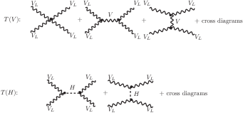
     (b)

Figure 1: (a) symbolic diagrams for weak boson scatterings. (b) the two kinds of scattering amplitudes $T(V)$ and $T(H)$ in weak boson scatterings.

In weak boson scatterings (cf. FIG. 1(a)), a quark $q_{1}$ in a proton becomes a forward jet $j^{f}_{1}$ (from the outgoing quark $q^{\prime}_{1}$) after emitting a weak boson. It can be seen from helicity analysis that, if $j^{f}_{1}$ and $j^{f}_{2}$ are sufficiently forward, the emitted weak bosons are mainly longitudinal. So that the ”initial state” weak bosons in FIG. 1 are $V_{L}$’s. Let us look at the longitudinal weak boson scatterings $V_{L}V_{L}\to V_{L}V_{L}$. At tree level, there are two kinds of weak boson scattering amplitudes shown in FIG. 1(b), namely the amplitude containing only gauge bosons $T(V)$, and the amplitude containing Higgs boson exchanges $T(H)$. Since the longitudinal polarization vector depends on the momentum of $V_{L}$, the two amplitudes $T(V)$ and $T(H)$ all depend on the center of mass energy $E$ as $E^{2}$. In the SM, the coupling constant between the Higgs boson and weak bosons in $T(H)$ is the same as the gauge coupling constant $g$ in $T(V)$. This makes the $E^{2}$-dependence terms in $T(V)$ and $T(H)$ exactly cancel in the total amplitude $T(V)+T(H)$, leading to a $E^{0}$-dependence of the total amplitude, which guarantees the unitarity of the $S$ matrix. In the case that the $HVV$ couplings in $T(H)$ are anomalous, the cancellation will not be exact, which leads to a $E^{2}$-dependence of the total amplitude. The magnitude of the remained $E^{2}$-dependence depends on the size of the anomalous couplings. So far as the anomalous couplings are within the unitarity bounds (4), there is no violation of the unitarity of the $S$ matrix below the new physics scale $\Lambda$. Thus in the high energy region of the LHC, the cross section is quite different from that in the SM. This is the reason why weak boson scatterings provide sensitive tests of the anomalous couplings. Different from the case of testing the strongly interacting EWSB mechanism in Ref. Bagger9495 , the signal in the present case is defined as the cross section with anomalous couplings $f_{n}\neq 0$ rather than the longitudinal cross section. So the $V_{L}V_{L}\to V_{L}V_{T},V_{T}V_{T}$ contributions with $f_{n}\neq 0$ are also signals. However, the transverse polarization vector is not momentum dependent, so that the $V_{L}V_{L}\to V_{L}V_{L}$ contribution with $f_{n}\neq 0$ is the most sensitive signal.

At the parton level, the signals and backgrounds in the gold-plated pure leptonic modes of weak boson scatterings have been studied systematically in Ref. Bagger9495 . Studying at the parton level, Ref. ZKHY03 showed that the $W^{+}_{L}W^{+}_{L}\to W^{+}_{L}W^{+}_{L}$ process is the most sensitive one for testing the anomalous couplings (6). Now we are going to study the semileptonic mode with $W^{+}W^{+}\to l^{+}\nu_{l}j_{1}j_{2}$. Since it is not possible to distinguish the jets from $W^{+}_{L}\to j_{1}j_{2}$ and $W^{-}_{L}\to j_{1}j_{2}$ experimentally, we have to take account of both the $W^{+}_{L}W^{+}_{L}$ and $W^{+}_{L}W^{-}_{L}$ productions and tag the final state $W^{+}_{L}W^{\pm}_{L}\to l^{+}\nu_{l}j_{1}j_{2}$. So we are going to calculate the full tree level contributions to the process

$$pp\to W^{+}W^{\pm}j^{f}_{1}j^{f}_{2}\to l^{+}\nu_{l}j_{1}j_{2}j^{f}_{1}j^{f}_{2},$$ (8)

where $W^{+}$ and $W^{\pm}$ are on-shell. Now the final state contains four jets, namely the two forward jets $j^{f}_{1}j^{f}_{2}$ and the two jets $j_{1}j_{2}$ from $W^{\pm}$ decays, so that the parton level study is not sufficient for finding out the suitable kinematic cuts to suppress the large backgrounds.

In the following, we shall work at the hadron level, calculating the full tree level contributions to the signal and backgrounds using the helicity amplitude methods helicity and the package PYTHIA PYTHIA with its default fragmentation model. For the parton distribution functions, we take CTEQ6L CTEQ6L . For the reconstruction of the $W$ boson from the two jets $j_{1}j_{2}$, we take the cluster-type jet algorithm Catani , and using the package ALPGEN ALPGEN . We shall develop suitable kinematic cuts to suppress the backgrounds and save the signal as much as possible.

The backgrounds to $V_{L}V_{L}$ scatterings can be classified into three kinds, namely the EW background, the QCD background, and the top quark background Bagger9495 . The irreducible EW background amplitudes (with the same final state particles as the signal) should be calculated together with the signal amplitude to guarantee gauge invariance. Other backgrounds with different initial or final state particles can be calculated separately.

Let $\sigma(f_{n}\neq 0)$ and $\sigma_{B}\equiv\sigma(f_{n}=0)$ be the total and background cross sections, respectively. We define the signal cross section $\sigma_{S}$ by

$$\sigma_{S}\equiv\sigma(f_{n}\neq 0)-\sigma_{B}.$$ (9)

Now the main experimental interest is to find out new physics effect beyond the SM background. Let $N_{S}$ and $N_{B}$ be the numbers of the signal events and background events, respectively. For large values of $N_{S}$ and $N_{B}$, we determine the statistical significance $\sigma_{stat}$ according to

$$\sigma_{stat}=\frac{N_{S}}{\sqrt{N_{B}}}.$$ (10)

However, the simple expression (10) holds only when $N_{S}$ and $N_{B}$ are large. For general values of $N_{S}$ and $N_{B}$, (10) is not precise enough, and we should take the general Poisson probability distribution approach

$$\displaystyle P_{B} = \sum_{N}\displaystyle e^{-N_{B}}\frac{N_{B}^{N}}{N!},$$ (11)

$$N=N_{S}+N_{B},N_{S}+N_{B}+1,\cdots,\infty.$$

From the obtained value of $1-P_{B}$, we can find out the corresponding value of $\sigma_{stat}$ PDG . The value of $\sigma_{stat}$ obtained in this way approaches to that given in (10) when $N_{S}$ and $N_{B}$ are sufficiently large. We shall take the approach (11) throughout this paper.

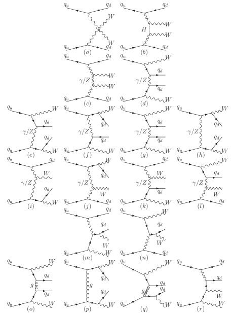
Figure 2: Typical Feynman diagrams for the signal and irreducible backgrounds in $W^{+}W^{+}$ scattering.

III Backgrounds and Cuts

Now we consider all the three kinds of backgrounds to $pp\to W^{+}W^{\pm}j^{f}_{1}j^{f}_{2}\to l^{+}\nu_{l}j_{1}j_{2}j^{f}_{1}j^{f}_{2}$, and study suitable kinematic cuts for suppressing them.

Considering the actual acceptance of the detectors at the LHC, we always require all the final state particles to be in the following rapidity range throughout this paper

$$|\eta|<4.5.$$ (12)

Recently, Ref. Butterworth provided a systematic hadron level study of the semileptonic modes in $WW$ scatterings at the LHC for testing the EW chiral Lagrangian coefficients when there are heavy resonances enhancing the scattering cross section at high energies. Although we assume there is no heavy resonances in our present case, the cross section is also enhanced at high energies by the energy dependence arising from the anomalous couplings. Thus the new techniques developed in Ref. Butterworth are also useful in our case. We shall apply some of their techniques to our study of testing the anomalous couplings of the light Higgs boson.

III.1 Signal and Irreducible Backgrounds

As mentioned above that the signal and irreducible background amplitudes should be put together in the calculation to guarantee gauge invariance. Take the $pp\to W^{+}W^{+}J^{f}_{1}j^{f}_{2}$ process as an example. The typical Feynman diagrams for these amplitudes are shown in FIG. 2 in which FIG. 2(b) (containing Higgs boson exchange) is the signal, and the total contribution of these diagrams with $f_{n}=0$ is the irreducible backgrounds.

The final state particles in the signal process contains two forward jets $j^{f}_{1}j^{f}_{2}$, two jets $j_{1}j_{2}$ from $W^{\pm}$ decays, a positively charged lepton $l^{+}$ and a missing neutrino $\nu_{l}$. Let us consider the cuts for each of the final state particles for extracting the signal.

III.1.1 Charged Lepton and Forward Jets

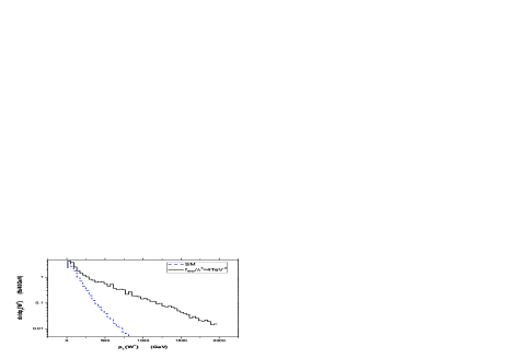
Figure 3: $d\sigma/dp_{T}(W^{+})$ distributions: The solid and dashed curves stand for the cases of $f_{WW}/\Lambda^{2}=4~{}{\rm TeV}^{-2},~{}f_{W}/\Lambda^{2}=0$ and $f_{WW}/\Lambda^{2}=f_{W}/\Lambda^{2}=0$, respectively.

Let us first consider the cut for the transverse momentum of the charged lepton $l^{+}$. Since the $W^{+}$ boson is quite energetic, the charged lepton $l^{+}$ moves almost along the direction of $W^{+}$. So we can look at the transverse momentum distribution of $W^{+}$. Take the case of $f_{WW}$ dominant as an example. FIG. 3 shows the transverse momentum distributions of the $W^{+}$ decaying into leptons with $f_{WW}/\Lambda^{2}=4~{}{\rm TeV}^{-2},f_{W}/\Lambda^{2}=0$ and with $f_{WW}/\Lambda^{2}=f_{W}/\Lambda^{2}=0$ (the irreducible background), respectively. We see that the distribution including the signal is significantly harder than that of the irreducible background. Thus we know that the transverse momentum distribution of the signal $l^{+}$ is significantly harder than that of the background $l^{+}$. From FIG. 3, we see that imposing the following $p_{T}(l^{+})$ cut can suppress the irreducible background and keep the signal as much as possible,

$$p_{T}(l^{+})>200~{}{\rm GeV}.$$ (13)

After the cut (13), the jets in most of the irreducible background processes are mainly in the low $|\eta|$ region. Thus imposing the requirement of the forward jets will effectively suppress this backgrounds. The observation of the tagging forward jets do not depend on whether we are testing the strongly interacting EWSB mechanism or testing the anomalous couplings of a light Higgs boson. So we can follow Ref. Butterworth to impose the following cuts on the transverse momentum $p_{T}(j^{f})$, the energy $E(j^{f})$, and the pseudorapidity $\eta(j^{f})$ of the two tagging forward jets Butterworth .

$$p_{T}(j^{f}_{i})>20~{}{\rm GeV},~{}~{}~{}~{}E(j^{f}_{i})>300~{}{\rm GeV},$$

$$2.0<|\eta(j^{f}_{i})|<4.5,~{}~{}i=1,2,$$

$$\eta(j^{f}_{1})\eta(j^{f}_{2})<0.$$ (14)

The rapidity cuts in (14) guarantee the two forward jets moving almost back-to-back. Later, we shall see that this forward jet cut will also suppress the $W+jets$ QCD background and the top quark background effectively. The efficiency of these cuts are listed in the second and third rows in TABLE 1. We see that the cuts (13) and (14) can suppress the irreducible background quite effectively.

III.1.2 Hadronic Decay of the $W$ boson

Now we come to the issue of extracting the $W^{\pm}\to j_{1}j_{2}$ events. Since the final state $W^{\pm}$ is very energetic, $98\%$ of the two jets $j_{1}j_{2}$ behave like a “single” energetic jet $J$ along the $W^{\pm}$ direction Butterworth , we first use the $k_{T}$ algorithm (the ALPGEN package ALPGEN ) with $E$ combination to pick up the most energetic “single jet”. Since $W^{\pm}$ and $W^{+}$ are almost back-to-back, we can impose the following cuts

$$p_{T}(J)>200~{}{\rm GeV},~{}~{}~{}~{}~{}~{}\eta(J)\eta(l^{+})<0,$$ (15)

and requiring the invariant mass $M_{J}$ to reconstruct the $W^{\pm}$ mass, i.e.

$$65~{}{\rm GeV}<M_{J}<95~{}{\rm GeV},$$ (16)

in which we have considered the realistic detection resolution $\pm 15$ GeV ATLAS .

III.2 QCD Backgrounds

One of the important QCD backgrounds is $pp\to W+\hat{n}$-parton which may leads to the final state $W+n$-jet at the hadron level. The case that three of the $n$ jets are detected (with other jets undetected), will be a background to the signal. We have examined the cases for $\hat{n}=1,2,3,4$ and found that the most important background comes from $\hat{n}=2$. Thus the main QCD background of this kind is

$$pp\to W+2{\rm-parton}\to W+3{\rm-jet}.$$ (17)

The typical Feynman diagrams for $qq,qg\to W+2{\rm-parton}$ are depicted in FIG. 4.

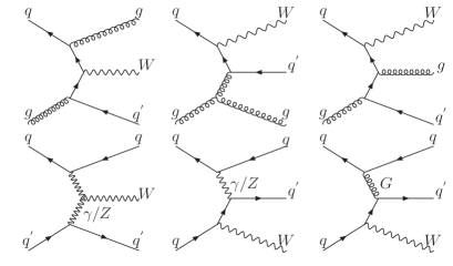
Figure 4: Typical diagrams for $W+$ 2-parton.

Another similar QCD background is

$$q\bar{q},qg,gg\to WW+n{\rm-jet}.$$ (18)

As mentioned above, the jets in the backgrounds (17) and (18) are less forward than the forward jets in the signal process when the lepton $l^{+}$ is constrained by (13). So imposing the cuts (13) and (14) can suppress these two kinds of QCD backgrounds effectively. Furthermore, the requirements (15) and (16) can significantly suppress this kind of background.

We can further impose a cut to suppress the above QCD backgrounds. The $y$ cut method (imposing a cut on $\log(p_{T}\sqrt{y})$) developed in Ref. Butterworth is very effective for this purpose. FIG. 5 shows the $\log(p_{T}\sqrt{y})$ distributions for the $pp\to W^{+}W^{\pm}j^{f}_{1}j^{f}_{2}$ (with $f_{W}/\Lambda^{2}=4$ GeV^-2) and $pp\to W+3{\rm-jet}$ processes.

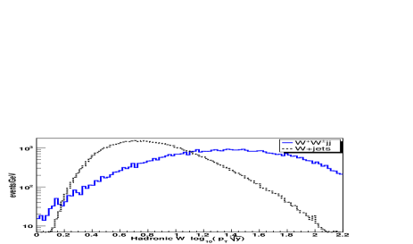
Figure 5: $\log(p_{T}\sqrt{y})$ distributions for the $pp\to W^{+}W^{\pm}j^{f}_{1}j^{f}_{2}$ and $pp\to W+3{\rm-jet}$ processes with $f_{W}/\Lambda^{2}=4$ TeV^-2, $f_{W}/\Lambda^{2}=0$.

From FIG. 5 we see that a cut Butterworth

$$1.6<\log(p_{T}\sqrt{y})<2.0$$ (19)

can effectively suppress the backgrounds. Indeed, after the cut (15), (16) and (19), the above QCD backgrounds are significantly reduced (cf. the fourth and fifth rows in TABLE 1).

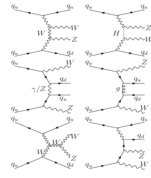
Figure 6: Typical diagrams for the $WZ+2$-$jet$ background.

There is also a kind of important QCD background which is the $WZjj$ process (cf. FIG. 6) since $M_{Z}$ is within the range in (16). This includes the $WZ$ scattering process, $pp\to W^{+}Zj^{f}_{1}j^{f}_{2}$, which is quite similar to the signal process $pp\to W^{+}W^{\pm}j^{f}_{1}j^{f}_{2}$. However, $M_{Z}$ is close to the upper bound in (16), i.e., a large portion of the tail of the $M_{Z}$ resonance higher than the peak is cut away by (16), so that the $WZ$ scattering background is significantly smaller than the signal. However, there are processes of this kind other than $WZ$ scattering (cf. FIG. 6) which can be large. We see from the fourth column of TABEL 1 that all the cuts imposed above can effectively suppress this kind of background.

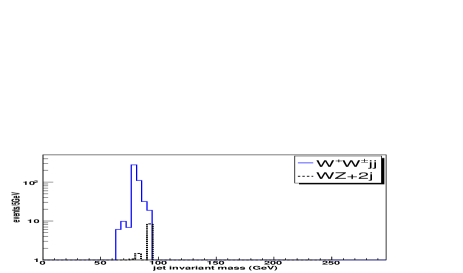
Figure 7: Reconstruction of the $W^{\pm}$ boson after the cuts (15) and (16). The solid curve is the $W^{\pm}$ peak in the signal process; the dashed curve shows the $Z$ boson peak in the $WZ+2{\rm-jet}$ background.

FIG. 7 shows the reconstructed $W$ boson peak in the signal process and the $Z$ boson peak in the $WZ$ scattering background after imposing the above cuts. We see that the $W$ boson peak is clearly reconstructed, and the $Z$ boson peak is significantly suppressed by the condition (16).

III.3 Top Quark Background

$W$ boson productions from the decay of top quarks in $t\bar{t}$ production (cf. FIG. 8) is an important background which mimics the signal.

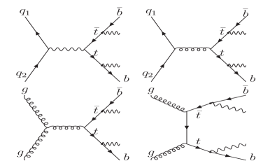
Figure 8: Typical diagrams for the $t\bar{t}$ background $gg\to t\bar{t}\to bW^{+}\bar{b}W^{-}$.

As mentioned above, the jets in this background are less forward than the two forward jets in the signal, so that the forward jet cuts (14) can suppress this background.

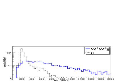
Figure 9: Invariant mass $M_{Jj}$ distributions for the top quark background (dashed curve) and the $pp\to W^{+}W^{\pm}j^{f}_{1}j^{f}_{2}$ process (solid curve).

However, further effective suppression is still needed. In the case of pure leptonic mode, this can be significantly suppressed by vetoing the central jets Bagger9495 . But in the semileptonic mode, the signal $W^{\pm}\to j_{1}j_{2}$ is in the central rapidity region, so that central jet veto cannot be applied. Ref. Butterworth considered the reconstruction of top quark, and eliminated this background by vetoing the events containing a top quark. Since we have already extracted the “single jet” $J$ of $j_{1}j_{2}$ satisfying the conditions (16) and (19), the momentum of the “single jet” can be measured. Then we can combine this “single jet” with the remaining jets $j$ (the $b$ jets) to reconstruct the top quark mass. FIG. 9 depicts the invariant mass $M_{Jj}$ distributions for the top quark background and the $pp\to W^{+}W^{\pm}j^{f}_{1}j^{f}_{2}$ process, which shows that we can extract the top quark peak by requiring Butterworth

$$130~{}{\rm GeV}<M_{Jj}<240~{}{\rm GeV}.$$ (20)

We do it event by event, and veto the events containing the top quark. This top quark veto requirement can further suppress the top quark background. The effect of this veto is listed in the sixth row in TABLE 1.

III.4 Additional Cuts

There are two commonly imposed additional cuts to suppress the backgrounds. The first one is the $p_{T}$ balance requirement TU-MSU08 (it is called hard $p_{T}$ in Ref. Butterworth ). Note that the signal process is a hard process in which the sum of the transverse momenta ($p_{T}$) of the final state particles vanishes ($p_{T}$ ballance). In the mentioned QCD backgrounds, there are undetected missing jets which carry $p_{T}$, so that summing up the $p_{T}$ of the detected final state particles will not vanish. Therefore imposing the requirement of $p_{T}$ balance can further suppress this kind of background. Considering the resolution of $p_{T}$ measurement ATLAS , we impose the following $p_{T}$ balance requirement TU-MSU08

$$\sum_{i}p^{i}_{T}<\pm 15~{}{\rm GeV},$$ (21)

where $p^{i}_{T}$ is the transverse momentum of the $i$th final state particle.

Another additional cut commonly used is called minijet veto. For the signal process, there is no color exchange between the forward jet quarks and the $W^{\pm}$ decay jet $J$. However, color exchange is expected in the background processes due to the remnant-remnant interactions, which can produce minijets. Therefore one can impose the additional cut of minijet veto by vetoing the events containing jets other than the signal jet $J$ from $W^{\pm}$ decay [satisfying (15) and (16)] in the central rapidity region, $|\eta|<2$ Butterworth .

The efficiencies of these additional cuts are shown in the last two rows in TABLE 1.

Table 1: Cut efficiency of the cross sections (in fb) for the signal with irreducible background (IB) and other backgrounds with the Higgs boson mass $m_{H}=115$ GeV, and the anomalous coupling $f_{W}/\Lambda^{2}=4.0~{}\text{TeV}^{-2}$ (with other anomalous couplings vanishing) as an example.

Cuts signal with IB IB ($f_{W}=0$) WZ+2-jet W+3-jet $t\bar{t}$ Without cuts 210.66 338.82 1431.67 2908923 407776.84 Eq. (13) 34.55 36.08 36.93 9630.86 2586.47 Eq. (14) 11.29 9.44 2.40 104.25 61.77 Eqs. (15) and (16) 7.01 4.12 0.12 0.10 1.09 Eq. (19) 2.42 1.29 2.7$\times{10^{-2}}$ 6.1$\times{10^{-3}}$ 0.09 Eq. (20) and top quark veto 2.39 1.27 2.3$\times{10^{-2}}$ 4.7$\times{10^{-3}}$ 0.06 Eq. (21) 2.28 1.26 5$\times{10^{-4}}$ 2$\times{10^{-4}}$ 2$\times{10^{-3}}$ Minijet veto 2.28 1.26 - - -

To illustrate the efficiencies of all these cuts, we list the cross sections (in fb) for the signal with irreducible background (IB), IB (obtained from the same process but with $f_{W}=0$), the QCD backgrounds, and the top quark background in TABLE 1 for $m_{H}=115$ GeV and $f_{W}/\Lambda^{2}=4$ TeV^-2 (with other anomalous couplings vanishing) as an example. We see that the cuts can significantly suppress the backgrounds. TABLE 1 shows that minijet veto does not affect the results much because the above cuts have already very efficiently suppressed the backgrounds. After the cuts, the main remained background is the irreducible background which is similar to the signal but is not enhanced at high energies by the momentum dependence of the anomalous couplings.

IV Numerical Results

From (6) we see that the anomalous couplings $g^{(i)}_{HVV}$ ($i=1,2$, $V$ stands for $\gamma,~{}W^{\pm},~{}Z^{0}$) are related to four parameters, namely $f_{W},~{}f_{WW},~{}f_{B},~{}f_{BB}$. For the process $pp\to W^{+}W^{\pm}j^{f}_{1}j^{f}_{2}$, except for the small contributions related to the photon, the main contributions are from the anomalous couplings of the Higgs boson to the weak gauge bosons, which is mainly contributed by $f_{W}$ and $f_{WW}$ since the contributions from $f_{B}$ and $f_{BB}$ are suppressed by a factor of $\sin^{2}\theta_{W}$ or $\sin^{4}\theta_{W}$ [cf. Eq. (6)]. In the following, we only take account of the contributions related to $f_{W}$ and $f_{WW}$, and neglect the $f_{B}$ and $f_{BB}$ contributions (setting $f_{B},f_{BB}=0$). With the above kinematic cuts, We give a full tree level calculation of the signal and background cross sections, event numbers, statistical significance [using Eq. (11)] for several values of integrated luminosity with various values of $f_{W}/\Lambda^{2}$ and $f_{WW}/\Lambda^{2}$ for $m_{H}$=115, 160, and 200 GeV. In this paper, we only take into account the statistical uncertainty. The issue related to the systematic error is beyond the scope of this paper, and we leave it to the experimentalists.

For simplicity, we first make a one-parameter study, i.e., considering the cases of $f_{W}/\Lambda^{2}$ dominant and $f_{WW}/\Lambda^{2}$ dominant separately. We shall discuss the two-parameter study in the end of this section.

Table 2: Cross sections (in fb) for $pp\rightarrow W^{+}W^{\pm}j^{f}_{1}j^{f}_{2}\rightarrow l^{+}\nu_{l}j_{1}j_{2}j^{f}_{1}j^{f}_{2}$ ($l^{+}=e^{+},\mu^{+}$) at the LHC with various values of $f_{W}/\Lambda^{2}$ and $\ f_{WW}/\Lambda^{2}$ (in TeV^-2) for $m_{H}=115,~{}160$ and 200 GeV.

$m_{H}$ (GeV)					$\displaystyle\frac{f_{W}}{\Lambda^{2}}$ (TeV-2)
	-4.0	-3.0	-2.0	-1.0	0	1.0	2.0	3.0	4.0
115	3.23	2.91	1.26	1.06	1.19	1.18	1.51	1.82	2.28
160	1.65	1.32	1.15	1.13	1.22	1.43	1.65	1.77	2.18
200	1.93	1.86	1.80	1.79	1.82	2.30	2.43	2.53	2.66
$m_{H}$ (GeV)					$\displaystyle\frac{f_{WW}}{\Lambda^{2}}$ (TeV${}^{-2})$
	-4.0	-3.0	-2.0	-1.0	0	1.0	2.0	3.0	4.0
115	4.88	3.11	1.66	1.37	1.19	1.34	2.04	3.34	5.36
160	12.35	4.48	2.10	1.36	1.22	1.64	2.70	4.12	6.90
200	11.50	5.61	3.27	2.11	1.82	2.26	2.74	4.46	6.94

First, we list in TABLE 2 the obtained cross sections with various values of $f_{W}/\Lambda^{2}$ and $f_{WW}/\Lambda^{2}$ (in TeV^-2) for $m_{H}$=115, 160, and 200 GeV. Note that the positive and negative regions of $f_{W}/\Lambda^{2}$ and $f_{WW}/\Lambda^{2}$ are not symmetric due to the interference between the signal and irreducible background amplitudes. We see that the cross sections are of the order of 1 fb which are larger than those in the pure leptonic mode [$O(0.1~{}{\rm fb})$] ZKHY03 by and order of magnitude. The largeness of the cross sections is due to: (i) the branching ratio for $W\to j_{1}j_{2}$ is larger than that for $W\to l^{+}\nu_{l}$, and (ii) we have included the process $pp\to W^{+}W^{-}j^{f}_{1}j^{f}_{2}\to l^{+}\nu_{l}j_{1}j_{2}j^{f}_{1}j^{f}_{2}$ as well, and with the improved cuts.

From TABLE 2 we see that for an integrated luminosity of 100 fb^-1, there can be of $O(10^{2})$ events detected at the LHC. This not only reduces the statistical uncertainty relative to that in the pure leptonic mode, but also provides the possibility of measuring the differential cross sections. This is the advantage of the semileptonic mode.

Next, we take an integrated luminosity of ${\cal L}_{int}\equiv\int dt{\cal L}=100$ fb^-1 to calculated the event numbers and using the approach of Eq. (11) to find out the sensitivities of $f_{W}/\Lambda^{2}$ and $\ f_{WW}/\Lambda^{2}$ (in TeV^-2) [and the related $g^{(i)}_{HVV}$ (in TeV^-1) in Eq. (6)] corresponding to the statistical significance of $1\sigma,~{}2\sigma$ and $3\sigma$ for $m_{H}=115,~{}160$ and 200 GeV. The results are listed in Eqs. (22), (23), and (24).

For $m_{H}=115$ GeV and ${\cal L}_{int}=100$ fb^-1 ($f_{W}/\Lambda^{2}$, $f_{WW}/\Lambda^{2}$ in TeV^-2, $g^{(i)}_{HVV}$ in TeV^-1), the results are:

$$\hbox{}1\sigma:$$

$$\hbox{}-2.0<f_{W}/\Lambda^{2}<1.2,~{}~{}-0.4<f_{WW}/\Lambda^{2}<0.8,~{}~{}~{}~{}$$

$$\hbox{}-0.053<g^{(1)}_{HWW}<0.032,~{}-0.042<g^{(2)}_{HWW}<0.021,$$

$$\hbox{}-0.053<g^{(1)}_{HZZ}<0.032,~{}~{}-0.016<g^{(2)}_{HZZ}<0.008,$$

$$\hbox{}-0.029<g^{(1)}_{HZ\gamma}<0.017,~{}~{}-0.018<g^{(2)}_{HZ\gamma}<0.009,$$

$$\hbox{}-0.005<g_{H\gamma\gamma}<0.002.$$

$$\hbox{}2\sigma:$$

$$\hbox{}-2.2<f_{W}/\Lambda^{2}<1.6,~{}~{}-1.1<f_{WW}/\Lambda^{2}<1.1,$$

$$\hbox{}-0.058<g^{(1)}_{HWW}<0.042,~{}-0.058<g^{(2)}_{HWW}<0.058,$$

$$\hbox{}-0.058<g^{(1)}_{HZZ}<0.042,~{}~{}-0.022<g^{(2)}_{HZZ}<0.022,$$

$$\hbox{}-0.032<g^{(1)}_{HZ\gamma}<0.023,~{}~{}-0.024<g^{(2)}_{HZ\gamma}<0.024,$$

$$\hbox{}-0.007<g_{H\gamma\gamma}<0.007.$$

$$\hbox{}3\sigma:$$

$$\hbox{}-2.4<f_{W}/\Lambda^{2}<1.9,~{}~{}-1.5<f_{WW}/\Lambda^{2}<1.3,$$

$$\hbox{}-0.063<g^{(1)}_{HWW}<0.050,~{}-0.068<g^{(2)}_{HWW}<0.079,$$

$$\hbox{}-0.063<g^{(1)}_{HZZ}<0.050~{}~{}-0.026<g^{(2)}_{HZZ}<0.030,$$

$$\hbox{}-0.035<g^{(1)}_{HZ\gamma}<0.027,~{}~{}-0.029<g^{(2)}_{HZ\gamma}<0.033,$$

$$\hbox{}-0.008<g_{H\gamma\gamma}<0.009.$$ (22)

For $m_{H}=160$ GeV and ${\cal L}_{int}=100$ fb^-1 ($f_{W}/\Lambda^{2}$, $f_{WW}/\Lambda^{2}$ in TeV^-2, $g^{(i)}_{HVV}$ in TeV^-1), the results are:

$$\hbox{}1\sigma:$$

$$\hbox{}-2.7<f_{W}/\Lambda^{2}<0.3,~{}~{}-0.9<f_{WW}/\Lambda^{2}<0.2,$$

$$\hbox{}-0.071<g^{(1)}_{HWW}<0.008,~{}-0.011<g^{(2)}_{HWW}<0.047,$$

$$\hbox{}-0.071<g^{(1)}_{HZZ}<0.008,~{}~{}-0.004<g^{(2)}_{HZZ}<0.018,$$

$$\hbox{}-0.039<g^{(1)}_{HZ\gamma}<0.004,~{}~{}-0.004<g^{(2)}_{HZ\gamma}<0.020,$$

$$\hbox{}-0.001<g_{H\gamma\gamma}<0.005.$$

$$\hbox{}2\sigma:$$

$$\hbox{}-3.4<f_{W}/\Lambda^{2}<0.9,~{}~{}-1.1<f_{WW}/\Lambda^{2}<0.5,$$

$$\hbox{}-0.089<g^{(1)}_{HWW}<0.024,~{}-0.026<g^{(2)}_{HWW}<0.058,$$

$$\hbox{}-0.089<g^{(1)}_{HZZ}<0.024,~{}~{}-0.010<g^{(2)}_{HZZ}<0.022,$$

$$\hbox{}-0.049<g^{(1)}_{HZ\gamma}<0.013,~{}~{}-0.011<g^{(2)}_{HZ\gamma}<0.024,$$

$$\hbox{}-0.003<g_{H\gamma\gamma}<0.007.$$

$$\hbox{}3\sigma:$$

$$\hbox{}-3.8<f_{W}/\Lambda^{2}<1.5,~{}~{}-1.3<f_{WW}/\Lambda^{2}<0.8,$$

$$\hbox{}-0.100<g^{(1)}_{HWW}<0.039,~{}-0.042<g^{(2)}_{HWW}<0.068,$$

$$\hbox{}-0.100<g^{(1)}_{HZZ}<0.039~{}~{}-0.016<g^{(2)}_{HZZ}<0.026,$$

$$\hbox{}-0.055<g^{(1)}_{HZ\gamma}<0.022,~{}~{}-0.018<g^{(2)}_{HZ\gamma}<0.029,$$

$$\hbox{}-0.005<g_{H\gamma\gamma}<0.008.$$ (23)

For $m_{H}=200$ GeV and ${\cal L}_{int}=100$ fb^-1 ($f_{W}/\Lambda^{2}$, $f_{WW}/\Lambda^{2}$ in TeV^-2, $g^{(i)}_{HVV}$ in TeV^-1), the results are:

$$\hbox{}1\sigma:$$

$$\hbox{}-3.2<f_{W}/\Lambda^{2}<0.2,~{}~{}-0.7<f_{WW}/\Lambda^{2}<0.2,$$

$$\hbox{}-0.084<g^{(1)}_{HWW}<0.005,~{}-0.011<g^{(2)}_{HWW}<0.037,$$

$$\hbox{}-0.084<g^{(1)}_{HZZ}<0.005~{}~{}-0.004<g^{(2)}_{HZZ}<0.014,$$

$$\hbox{}-0.046<g^{(1)}_{HZ\gamma}<0.003,~{}~{}-0.004<g^{(2)}_{HZ\gamma}<0.015,$$

$$\hbox{}-0.001<g_{H\gamma\gamma}<0.004.$$

$$\hbox{}2\sigma:$$

$$\hbox{}-4.1<f_{W}/\Lambda^{2}<0.6,~{}~{}-1.0<f_{WW}/\Lambda^{2}<0.7,$$

$$\hbox{}-0.108<g^{(1)}_{HWW}<0.016,~{}-0.037<g^{(2)}_{HWW}<0.053,$$

$$\hbox{}-0.108<g^{(1)}_{HZZ}<0.016,~{}~{}-0.014<g^{(2)}_{HZZ}<0.020,$$

$$\hbox{}-0.059<g^{(1)}_{HZ\gamma}<0.009,~{}~{}-0.015<g^{(2)}_{HZ\gamma}<0.022,$$

$$\hbox{}-0.004<g_{H\gamma\gamma}<0.006.$$

$$\hbox{}3\sigma:$$

$$\hbox{}-4.3<f_{W}/\Lambda^{2}<0.8,~{}~{}-1.2<f_{WW}/\Lambda^{2}<1.0,$$

$$\hbox{}-0.113<g^{(1)}_{HWW}<0.021,~{}-0.053<g^{(2)}_{HWW}<0.063,$$

$$\hbox{}-0.113<g^{(1)}_{HZZ}<0.021~{}~{}-0.020<g^{(2)}_{HZZ}<0.024,$$

$$\hbox{}-0.062<g^{(1)}_{HZ\gamma}<0.012,~{}~{}-0.022<g^{(2)}_{HZ\gamma}<0.027,$$

$$\hbox{}-0.006<g_{H\gamma\gamma}<0.007.$$ (24)

Eq. (22) is to be compared with the sensitivities in the pure leptonic mode with $m_{H}=115$ GeV for an integrated luminosity of 300 fb ^-1 ($f_{W}/\Lambda^{2}$ and $f_{WW}/\Lambda^{2}$ are in TeV^-2) ZKHY03 .

$$\hbox{}1\sigma:$$

$$\hbox{}-1.0<f_{W}/\Lambda^{2}<0.85,~{}~{}-1.6<f_{WW}/\Lambda^{2},1.6,$$

$$\hbox{}2\sigma:$$

$$\hbox{}-1.4<f_{W}/\Lambda^{2}<1.2,~{}~{}-2.2<f_{WW}/\Lambda^{2}<2.2,$$

$$\hbox{}3\sigma:$$

$$\hbox{}-1.7<f_{W}/\Lambda^{2}<1.6,~{}~{}-2.9<f_{WW}/\Lambda^{2}<2.9.$$ (25)

Note that $f_{W}/\Lambda^{2}$ is more sensitive in the pure leptonic mode, while $f_{WW}/\Lambda^{2}$ is more sensitive in the semileptonic mode. This is because that the process considered in the pure leptonic mode is only $pp\to W^{+}W^{+}j^{f}_{1}j^{f}_{2}$, while it is $pp\to W^{+}W^{\pm}j^{f}_{1}j^{f}_{2}$ in the semileptonic mode. Anyway, the $2\sigma$ sensitivities in the two modes are of the same level. Since the required integrated luminosity in the pure leptonic mode is 300 fb^-1 while it is only 100 fb^-1 in the semileptonic mode, the semileptonic mode can reduce the required integrated luminosity by a factor of 3 relative to the pure leptonic mode. So the anomalous couplings can be measured to this sensitivity when the LHC reaches its designed luminosity, 100 fb^-1/year, or even earlier. This is quite promising.

Table 3: Numbers of events for $pp\rightarrow W^{+}W^{\pm}j^{f}_{1}j^{f}_{2}\rightarrow l^{+}\nu_{l}j_{1}j_{2}j^{f}_{1}j^{f}_{2}$ ($l^{+}=e^{+},\mu^{+}$) at the LHC for an integrated luminosity of 50 fb^-1 with various values of $f_{W}/\Lambda^{2}$ and $\ f_{WW}/\Lambda^{2}$ (in TeV^-2) for $m_{H}=115,~{}160$ and 200 GeV. The values of the statistical significance $\sigma_{stat}$ are shown in the parentheses.

$m_{H}$ (GeV)					$\displaystyle\frac{f_{W}}{\Lambda^{2}}$ (TeV-2)
	-4.0	-3.0	-2.0	-1.0	0	1.0	2.0	3.0	4.0
115	162 (13.21)	146 (11.16)	63 (0.81)	53 (-)	60 (0)	59 (-)	76 (2.12)	91 (4.05)	114 (7.09)
160	83 (2.75)	66 (1.09)	58 (-)	57 (-)	61 (0)	72 (1.58)	83 (2.75)	89 (3.50)	109(6.09)
200	96 (1.01)	93 (0.79)	90 (-)	89 (-)	91 (0)	115 (2.54)	121 (3.18)	126 (3.71)	133 (4.39)
$m_{H}$ (GeV)					$\displaystyle\frac{f_{WW}}{\Lambda^{2}}$ (TeV-2)
	-4.0	-3.0	-2.0	-1.0	0	1.0	2.0	3.0	4.0
115	244 (23.89)	156 (12.41)	83 (3.06)	69 (1.39)	60 (0)	67 (1.28)	102 (5.51)	167 (13.91)	268 (26.99)
160	618 (71.13)	224 (20.85)	105 (5.61)	68 (1.18)	62 (0)	82 (2.75)	135 (9.42)	206 (18.52)	345 (36.30)
200	575 (50.14)	281 (19.56)	164 (7.39)	106 (1.56)	93 (0)	113 (2.17)	137 (4.64)	223 (13.56)	347 (26.44)

So far we have concentrated on the study of the detection sensitivities. In the real world, the actual anomalous coupling(s) might be larger than the sensitivity bound(s) given above. So nonvanishing anomalous coupling(s) might even be detected for lower integrated luminosities at the LHC. Let us take the integrated luminosity of 50 fb^-1 as an example. In TABLE 3, we list the numbers of events for $pp\rightarrow W^{+}W^{\pm}j^{f}_{1}j^{f}_{2}\rightarrow l^{+}\nu_{l}j_{1}j_{2}j^{f}_{1}j^{f}_{2}$ at the LHC for an integrated luminosity of 50 fb^-1 with various values of $f_{W}/\Lambda^{2}$ and $\ f_{WW}/\Lambda^{2}$ (in TeV^-2) for $m_{H}=115,~{}160$ and 200 GeV. The values of the statistical significance $\sigma_{stat}$ are shown in the parentheses.

Our calculation shows that the sensitivity bounds for $m_{H}=115\--200$ GeV and ${\cal L}_{int}=50$ fb^-1 are:

$$1\sigma:$$

$$~{}~{}~{}~{}-3.5~{}{\rm TeV}^{-2}\leq f_{W}/\Lambda^{2}\leq 1.3~{}{\rm TeV}^{-2},$$

$$~{}~{}~{}~{}-0.9~{}{\rm TeV}^{-2}\leq f_{WW}/\Lambda^{2}\leq 0.8~{}{\rm TeV}^{-2},$$

$$3\sigma:$$

$$~{}~{}~{}~{}-4.5~{}{\rm TeV}^{-2}\leq f_{W}/\Lambda^{2}\leq 2.4~{}{\rm TeV}^{-2},$$

$$~{}~{}~{}~{}-2.0~{}{\rm TeV}^{-2}\leq f_{WW}/\Lambda^{2}\leq 1.5~{}{\rm TeV}^{-2}.$$ (26)

If the anomalous coupling constants in the nature are beyond the $1\sigma$ bounds in (26), the LHC can already detect their effect with several tens to a hundred of events when the integrated luminosity reaches 50 fb^-1. This is quite promising since it can be started within the first couple of years run of the LHC. If they are beyond the $3\sigma$ bounds, the LHC can perform a $3\sigma$ detection for an integrated luminosity of 50 fb^-1. If the experiment does not find the evidence of the anomalous couplings at the LHC for an integrated luminosity of 50 fb^-1, it means that $f_{W}/\Lambda^{2}$ and $f_{WW}/\Lambda^{2}$ are within the $1\sigma$ sensitivity bounds given in (26), and further detection with higher integrated luminosity is needed.

Finally we show some results of the two-parameter study.

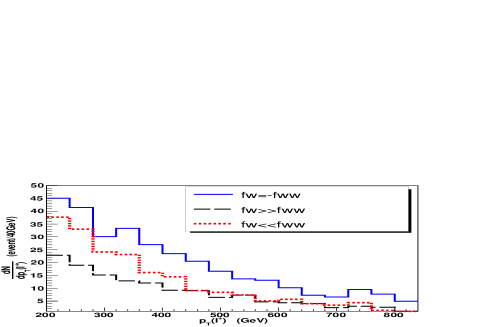
Figure 10: Leptom transverse momentum distributions in the case of $m_{H}=115$ GeV for an integrated luminosity of 100 fb^-1 taking the cases of $f_{W}/\Lambda^{2}=2~{}{\rm TeV}^{-2}\gg f_{WW}/\Lambda^{2},~{}f_{WW}/\Lambda^{2}=2~{}{\rm TeV}^{-2}\gg f_{W}/\Lambda^{2}$ and $f_{W}/\Lambda^{2}=-f_{WW}/\Lambda^{2}=2~{}{\rm TeV}^{-2}$ as examples.

As mentioned above, with the large cross sections in the semileptonic mode, we can study differential cross sections which behave differently for different values of $f_{W}$ and $f_{WW}$, so that we can determine $f_{W}$ and $f_{WW}$ separately from this information. As an example, we plot, in FIG. 10, the $p_{T}(l^{+})$ distributions for $m_{H}=115$ GeV and ${\cal L}_{int}$=100 fb^-1 contributed by three different sets of $f_{W}/\Lambda^{2}$ and $f_{WW}/\Lambda^{2}$ from different regions in the two-parameter space, namely the cases of $f_{W}/\Lambda^{2}=2~{}{\rm TeV}^{-2}\gg f_{WW}/\Lambda^{2},~{}f_{WW}/\Lambda^{2}=2~{}{\rm TeV}^{-2}\gg f_{W}/\Lambda^{2}$, and $f_{W}/\Lambda^{2}=-f_{WW}/\Lambda^{2}=2~{}{\rm TeV}^{-2}$. We see that the three $p_{T}(l^{+})$ distributions are different and quite distinguishable especially in the region near 200 GeV. Since the cross section is more sensitive to $f_{WW}/\Lambda^{2}$ than to $f_{W}/\Lambda^{2}$, the curve of the $f_{WW}/\Lambda^{2}=2~{}{\rm TeV}^{-2}\gg f_{W}/\Lambda^{2}$ case lies significantly higher than that of the $f_{W}/\Lambda^{2}=2~{}{\rm TeV}^{-2}\gg f_{WW}/\Lambda^{2}$ case. From Eq. (6) we see that $f_{W}/\Lambda^{2}$ appears in the formulae always with a positive sign, while $f_{WW}/\Lambda^{2}$ appears always with a negative sign. So that in the case of $f_{W}/\Lambda^{2}=-f_{WW}/\Lambda^{2}=2~{}{\rm TeV}^{-2}$, these two contributions are constructive, and thus this curve lies well above the two former curves. Therefore measuring both the cross section and the the $p_{T}(l^{+})$ distribution may help to separately determine the two parameters $f_{W}$ and $f_{WW}$ to a certain precision. If there is no characteristic signal for new physics model found before this measurement, the values of $f_{W}$ and $f_{WW}$ may serve as a clue for probing the underlying theory of new physics. This is an advantage of the semileptonic mode over the pure leptonic mode.

V Conclusion

In this paper, we have given a full tree level study of the test of anomalous gauge couplings [cf. Eqs. (1) and (6)] at the LHC via the $WW$ scattering processes $pp\to W^{+}W^{+}j^{f}_{1}j^{f}_{2}$ and $pp\to W^{+}W^{-}j^{f}_{1}j^{f}_{2}$ in the semileptonic mode $W^{+}\to l^{+}\nu_{l},~{}W^{+}~{}(W^{-})\to j_{1}j_{2}$. Through out this paper, we take into account only the statistical uncertainty. The issue of systematic error is beyond the scope of this paper, and we leave it to the experimentalists.

Both signals and backgrounds are calculated at the hadron level with suitably imposed kinematic cuts to suppress the backgrounds. As we mentioned in Sec. III-A, the signal and irreducible background should to calculated together to guarantee gauge invariance. The efficiencies of the cuts are shown in TABLE 1 which shows that the cuts (13)$\--$(21) can suppress the QCD backgrounds and the $t\bar{t}$ background quite efficiently. After the cuts, the main background remained is the irreducible background.

The obtained cross sections for $m_{H}=115,~{}160$ and 200 GeV in the ranges $|f_{W}/\Lambda^{2}|\leq 4$ and $|f_{WW}/\Lambda^{2}|\leq 4$ are listed in TABLE 2. Because of the largeness of the branching ratio $B(W^{\pm}\to j_{1}j_{2})$, the contributions of both $pp\to W^{+}W^{+}j^{f}_{1}j^{f}_{2}$ and $pp\to W^{+}W^{-}j^{f}_{1}j^{f}_{2}$, and the improved cuts, the cross sections are as large as of $O({\rm 1\,fb})\--O(10\,{\rm fb})$. So that for an integrated luminosity of 100 fb^-1, hundreds of events can be detected at the LHC.

As mentioned in Sec. IV that the $pp\to W^{+}W^{\pm}j^{f}_{1}j^{f}_{2}$ processes are mainly sensitive to two anomalous coupling constants, $f_{W}/\Lambda^{2}$ and $f_{WW}/\Lambda^{2}$. We first made a one-parameter study, i.e., considering the cases of $f_{W}/\Lambda^{2}$ dominant and $f_{WW}/\Lambda^{2}$ dominant separately. Taking the integrated luminosity of 100 fb^-1 as an example, the obtained results of the sensitivity ranges of $f_{W}/\Lambda^{2}$, $f_{WW}/\Lambda^{2}$ and the corresponding $g^{(i)}_{HVV}$’s for $1\sigma,~{}2\sigma$ and $3\sigma$ detections are listed in Eqs. (22) to (24) for $m_{H}=115$ GeV, 160 GeV and 200 GeV. These are of the same level as those in the pure leptonic mode for an integrated luminosity of 300 fb^-1. Thus for the same level of sensitivity, the semileptonic mode can reduce the required integrated luminosity by a factor of 3.

If the actual anomalous coupling constants in nature are not so small, it can even be measured with a low luminosity as 50 fb^-1. The obtained event numbers and statistical significance $\sigma_{stat}$ for an luminosity of 50 fb^-1 are listed in TABLE 3 which shows that a detection with around $O(100)$ events can be performed at the LHC for an integrated luminosity of 50 fb^-1 if the anomalous coupling constants in the nature are larger than the $1\sigma$ bounds given in Eq. (26). This can be done within the first couple of years run of the LHC. So it is quite promising. If the detected result is consistent with the SM value at the LHC for an integrated luminosity of 50 fb^-1, it means that $f_{W}/\Lambda^{2}$ and $f_{WW}/\Lambda^{2}$ are within the $1\sigma$ sensitivity bounds (26), and further detection with higher integrated luminosity is needed.

We have also made a simple two-parameter study considering $f_{W}/\Lambda^{2}$ and $f_{WW}/\Lambda^{2}$ simultaneously. With the hundreds of events for ${\cal L}_{int}=100$ fb^-1, it is possible to measure the $p_{T}$ distribution of the charged lepton experimentally. We plotted in FIG. 10 the $p_{T}(l^{+})$ distributions for $m_{H}=115$ GeV and ${\cal L}_{int}=100$ fb^-1 corresponding to $f_{W}/\Lambda^{2}=2\,{\rm TeV}^{-2}\gg f_{WW}/\Lambda^{2},~{}f_{WW}/\Lambda^{2}=2\,{\rm TeV}^{-2}\gg f_{W}/\Lambda^{2}$, and $f_{W}/\Lambda^{2}=-f_{WW}/\Lambda^{2}=2\,{\rm TeV}^{-2}$ as examples. It shows that the three distributions are quite distinguishable. Therefore measuring both the total cross section and the $p_{T}(l^{+})$ distribution may determine the two parameters $f_{W}/\Lambda^{2}$ and $f_{WW}/\Lambda^{2}$ separately to certain precision. This may provide a clue for figuring out the underlying theory of new physics beyond the SM if no other characteristic signal of the new physics is found before that measurement.

In summary, the process $pp\to W^{+}W^{\pm}j^{f}_{1}j^{f}_{2}\to l^{+}\nu_{l}j_{1}j_{2}j^{f}_{1}j^{f}_{2}$ at the LHC can provide a sensitive test of the anomalous gauge couplings of the Higgs boson showing the effect of new physics beyond the SM. The experiment can start the test for an integrated luminosity around 50 fb^-1, and can measure the total cross section and the $p_{T}$ distributions of the charged lepton to certain precision for an integrated luminosity of 100 fb^-1. With such measurements, it is possible to determine the two main parameters $f_{W}/\Lambda^{2}$ and $f_{WW}/\Lambda^{2}$ of the anomalous couplings separately, which may provide a clue for figuring out the underlying theory of new physics.

ACKNOWLEDGMENTS

We would like to thank Yuanning Gao for useful discussions. This work is supported by National Natural Science Foundation of China under Grant Nos. 10635030, 10875064, 10705017 and 10435040.

References

• (1) C. Amsler et al., (Particle Data Group), Phys. Lett. B 667, 1 (2008).
• (2) R. Dashen and H. Neuberger, Phys. Rev. Lett. 50, 1897 (1983).
• (3) L.Susskind, Phys. Rev. D 20, 2619 (1979).
• (4) K. Hagiwara, S. Ishihara, R. Szalapski, and D. Zeppenfeld, Phys. Rev. D 48, 2182 (1993).
• (5) W. Buchmüller and D. Wyler, Nucl. Phys. B 268, 621 (1986); C.J.C. Burgess and H.J. Schnitzer, Nucl. Phys. B 228, 464 (1983); C.N. Leung, S.T. Love, and S. Rao, Z. Phys. C 31, 433 (1986).
• (6) For a review, see M.C. Gonzalez-Garcia, Int. J. Mod. Phys. A 14, 3121 (1999).
• (7) R. Sekhar Chivukula and V. Koulovassilopouplos, Phys. Lett. B 309, 371 (1993).
• (8) Bin Zhang, Yu-Ping Kuang, Hong-Jian He, and C.-P. Yuan, Phys. Rev. D 67, 114024 (2003).
• (9) V. Barger, T. Han, P. Langacker, B. McEltrath, and P.M. Zerwas, Phys. Re. D 67, 115001 (2003).
• (10) G.J. Gounaris, J. Layssac, and F.M. Renard, Phys. Lett. B 332,146 (1994); G.J. Gounaris, J. Layssac, J.E. Pascalis, and F.M. Renard, Z. Phys. C 66, 619 (1995).
• (11) O.J.P. Éboli, M.C. Gonzalez-Garcia, S.M. Lietti, and S.F. Novaes, Phys. Lett. B 478, 199 (2000); F. de Campos, M.C. Ganzalez-Garcia, S.M. Lietti, S.F. Novaes, and R. Rosenfeld, Phys. Lett. B 435, 407 (1998).
• (12) T. Plehn, D. Rainwater, and D. Zeppenfeld, Phys. Rev. Lett. 88, 051801 (2002).
• (13) E.g, V. Barger, K. Cheung, A. Djouadi, B.A. Kniel, and P. M. Zerwas, Phys. Rev. D 49, 79 (1994); M. Kramer, J. Kuhn, M. L. Stong and P. M. Zerwas, Z. Phys. C 64, 21 (1994); K. Hagiwara and M. Stong, Z. Phys. C 62, 99 (1994); J.F. Gunion, T. Han, and R. Sobey, Phys. Lett. B 429, 79 (1998); K. Hagiwara, S. Ishihara, J. Kamoshita, and B.A. Kniel, Eur. Phys. J. 14, 457 (2000).
• (14) T. Han, Y.-P. Kuang, and B. Zhang, Phys. Rev. D 73, 055010 (2006).
• (15) J.Bagger, V.Barger, K.Cheung, J.Gunion, T.Han, G.A.Ladinsky,R.Rosenfeld and C.-P.Yuan, Phys. Rev. D 49, 1246 (1994).Phys. Rev. D 52, 3878 (1995).
• (16) K.Hagiwara and D.Zeppenfeld, Nucl. Phys. B 313, 560 (1989); V. Barger, T. Han, and D. Zeppenfeld, Phys. Rev. D 41, 2782 (1990).
• (17) T. Sjöstrand, P. Ed en, C. Friberg, L. Lönnblad, G. Miu, S. Mrenna and E. Norrbin, Computer Physics Commun 135, 238 (2001).
• (18) J. Pumplin, D.R. Stump, J. Huston, H.L. Lai, P. Nadolsky, W.K. Tung, J. High Energy Phys. 07, 012 (2002).
• (19) S. Cantani et al., Nucl. Phys. B 406, 187 (1993).
• (20) M.H.Seymour, Z. Phys. C 62, 127 (1994).
• (21) J.M. Butterworth, B.E. Cox, and J.R. Forshaw, Phys. Rev. D 65, 096014 (2002).
• (22) ATLAS Physics TDR, Detector and Physics Performance —Technical Design Reports. CERN/LHCC/99-15, vol. 1.
• (23) H.-J. He, Y.-P. Kuang, Y.-H. Qi, B. Zhang, A. Belyaev, R.S. Chivukula, N.D. Christensen, A. Pukhov, and E.H. Simmons, Phys. Rev. D 78, 031701(R) (2008).