Cross-correlations in scaling analyses of phase transitions

Abstract

Thermal or finite-size scaling analyses of importance sampling Monte Carlo time series in the vicinity of phase transition points often combine different estimates for the same quantity, such as a critical exponent, with the intent to reduce statistical fluctuations. We point out that the origin of such estimates in the same time series results in often pronounced cross-correlations which are usually ignored even in high-precision studies, generically leading to significant underestimation of statistical fluctuations. We suggest to use a simple extension of the conventional analysis taking correlation effects into account, which leads to improved estimators with often substantially reduced statistical fluctuations at almost no extra cost in terms of computation time.

With the advent of the renormalization group in the 1960s, the notions of scaling and universality have been combined into the solid basis of our understanding of critical phenomena in statistical physics, field theory and a wealth of applications in areas ranging from solid-state physics Chaikin and Lubensky (2000) to cosmology Bergström and Goobar (2004). It is through the remarkable fact that the most important properties of a continuous phase transition are independent of many microscopic details and, instead, only depend on a small number of fundamental characteristics of a system, such as the dimensionality and the symmetries of the order parameter, that we can accurately describe such different situations as, e.g., the liquid-vapor phase transition and the ferromagnetic transition of uniaxial magnets, with one and the same scaling theory. Recently, the investigation of quantum phase transitions has opened up a new Pandora’s box with a wealth of transitions partially defining novel universality classes Vojta (2003). The direct applicability of results from simple models to a range of experimentally realized systems implied by the principle of universality renders high-precision determinations of critical parameters for the most common universality classes a rewarding goal.

Particularly through the conception of advanced finite-size scaling (FSS) approaches and novel efficient algorithms Binder and Landau (2005), Monte Carlo (MC) simulations have grown up to become a tool for the determination of universal critical quantities clearly competitive compared to the more traditional approaches of high-temperature and field-theoretic expansions Pelissetto and Vicari (2002). Likewise, the detailed investigation of systems undergoing first-order phase transitions has become a classic application of the MC simulation technique Janke (2003). Major advances in the competitiveness of the MC method for these purposes came with the advent of histogram methods Ferrenberg and Swendsen (1988) and generalized-ensemble simulation techniques such as the multicanonical method Berg and Neuhaus (1992), both of which allow for extracting estimates of thermal averages for a continuous range of temperatures or other external parameters from a single MC simulation. It is only through this effective continuity of information that high-precision investigations of phase transitions have come into the reach of simulation methods. For arriving at high-precision estimates, however, all possible sources of error must be put under close scrutiny. This is often done to a high degree of sophistication concerning the systematic errors resulting from corrections to scaling Pelissetto and Vicari (2002) and the statistical errors resulting from the stochastic nature of MC time series (including their timewise autocorrelations for the case of the most commonly used Markov chain MC techniques) Berg (2004); Efron and Tibshirani (1998). It has not been systematically discussed previously, however, that the extraction of different estimates from a single time series in thermal or FSS analyses must entail cross-correlations. As will be shown below, neglecting their effect not only results in systematically wrong estimates of statistical errors, but also fails to fully exploit the available time-series data to yield the maximum statistical precision obtainable.

Although our considerations apply generally to all situations where a number of different estimates from the same (set of) simulation(s) are combined to a final result, for specificity we consider the FSS analysis of simulation data in the vicinity of a critical point. For the purpose of illustration we choose the technique outlined in Ref. Ferrenberg and Landau (1991), but very similar considerations apply to alternative approaches, see, e.g., Refs. Ballesteros et al. (1996); Hasenbusch (1999). To be specific, we here use a magnetic language and first consider the maxima of the derivative of the magnetization cumulants $U_{2k}=1-\langle|m|^{2k}\rangle/3\langle|m|^{k}\rangle^{2}$ for $k=1$, $2$, $\ldots$:

$$\left.\frac{\mathrm{d}U_{2k}}{\mathrm{d}\beta}\right|_{\mathrm{max}}=U_{k,0}L^{1/\nu}(1+U_{k,c}L^{-w}+\cdots),$$ (1)

where $L$ denotes the linear size of the system and $\beta$ is the inverse temperature. This relation allows for a precise determination of the correlation length exponent $\nu$ without previous knowledge of the critical temperature. In many cases at least some of the scaling corrections, such as an effective leading correction with exponent $w$ as indicated in Eq. (1), need to be taken into account to achieve the desired level of accuracy. An analogous relation holds for the scaling of the maxima of the logarithmic derivative of magnetization moments,

$$\left.\frac{\mathrm{d}\ln\langle|m|^{k}\rangle}{\mathrm{d}\beta}\right|_{\mathrm{max}}=D_{k,0}L^{1/\nu}(1+D_{k,c}L^{-w}+\cdots).$$ (2)

These scaling relations for determining $\nu$ only become useful as soon as the maximum values $\left.(\mathrm{d}U_{2k}/\mathrm{d}\beta)\right|_{\mathrm{max}}$ and $\left.(\mathrm{d}\ln\langle|m|^{k}\rangle/\mathrm{d}\beta)\right|_{\mathrm{max}}$ can be computed to high accuracy without the need for repeated simulations manually tracking their locations in $\beta$. In case of a histogram or reweighting analysis of a single canonical simulation, this is effected through the continuous family of estimates

$$\hat{A}(\beta)=\frac{\sum_{i}A_{i}e^{-(\beta-\beta_{0})E_{i}}}{\sum_{i}e^{-(\beta-\beta_{0})E_{i}}}$$ (3)

for the thermal average $\langle A\rangle_{\beta}$ from a time series $\{A_{i}\}$ of measurements resulting from an importance sampling simulation at inverse temperature $\beta_{0}$. Conventional techniques of numerical analysis such as a golden section search then allow for an efficient determination of the maxima of Eqs. (1) and (2) to high precision. Once $\nu$ has been determined, the scaling of the shifts of the location of the maxima of quantities such as $\mathrm{d}U_{2k}/\mathrm{d}\beta$ and $\mathrm{d}\ln\langle|m|^{k}\rangle/\mathrm{d}\beta$ as well as the specific heat, susceptibility etc. allow to locate the transition coupling $\beta_{c}$. Finally, the remaining critical exponents may be estimated from the FSS of the maxima of the specific heat to yield $\alpha/\nu$, of the susceptibility to yield $\gamma/\nu$ etc. Since the exponent $\nu$ enters all FSS relations, it clearly is of utmost importance to exploit the available data to their fullest for a precise estimate of $\nu$. In view of the family of relations (1) and (2), this certainly includes a combination of estimates from $\mathrm{d}U_{2k}/\mathrm{d}\beta$ and $\mathrm{d}\ln\langle|m|^{k}\rangle/\mathrm{d}\beta$ as well as from the different choices of the parameter $k$ Ferrenberg and Landau (1991).

To see how this combination should be performed, consider a number $n$ of different estimators $\hat{x}_{i}$ with the same expectation value (e.g., $\hat{x}_{i}=\hat{\nu}_{i}$). A combined average results from a linear combination $\bar{x}=\sum_{i}\alpha_{i}\hat{x}_{i}$ with $\sum_{i}\alpha_{i}=1$. While any such combination yields a valid estimator of $\langle x\rangle$, e.g., the arithmetic mean $\bar{x}_{\mathrm{plain}}$ with $\alpha_{i}=1/n$, the ensuing statistical fluctuations will be larger than necessary. For uncorrelated estimates $\hat{x}_{i}$ minimal variance of $\bar{x}$ is achieved for the error-weighted mean $\bar{x}_{\mathrm{err}}$ with Brandt (1998)

$$\alpha_{i}=Z^{-1}\frac{1}{\sigma^{2}(\hat{x}_{i})},$$ (4)

where $\sigma^{2}(\hat{x}_{i})$ denotes the variance of $\hat{x}_{i}$ and $Z=\sum_{i}1/\sigma^{2}(\hat{x}_{i})$. In general, however, the estimates $\hat{x}_{i}$, stemming from a reweighting analysis of the same MC time series, will be substantially correlated. Under these circumstances, the optimum choice is a covariance-weighted mean $\bar{x}_{\mathrm{cov}}$ with weights Brandt (1998); Janke and Sauer (1997)

$$\alpha_{i}=Z^{-1}\sum_{j}[\Gamma(\hat{x})^{-1}]_{ji},$$ (5)

where $\Gamma(\hat{x})^{-1}$ denotes the inverse of the covariance matrix $\Gamma_{ij}(\hat{x})=\langle\hat{x}_{i}\hat{x}_{j}\rangle-\langle\hat{x}_{i}\rangle\langle\hat{x}_{j}\rangle$ and $Z=\sum_{ij}[\Gamma(\hat{x})^{-1}]_{ij}$. Since for uncorrelated estimates $[\Gamma(\hat{x})^{-1}]_{ij}=\delta_{ij}/\sigma^{2}(\hat{x}_{i})$, Eq. (4) is recovered in this special case. Even more dramatically affected by correlations are the statistical errors of averages, where the standard formula $\sigma^{2}_{\mathrm{uncorr}}(\bar{x})=\sum_{i}\alpha_{i}^{2}\sigma^{2}(\hat{x}_{i})$ is no longer valid and must be modified to read $\sigma^{2}_{\mathrm{corr}}(\bar{x})=\sum_{i,j}\alpha_{i}\alpha_{j}\Gamma_{ij}(\hat{x})$, generically leading to an underestimate of fluctuations via the naive (and wrong) estimator $\sigma^{2}_{\mathrm{uncorr}}$.

To check for the strength of such correlation effects and their influence on finding optimal averages endowed with valid estimates of statistical errors, we performed a FSS analysis of the critical points of the ferromagnetic Ising model in two (2D) and three (3D) dimensions. Time series data for the configurational energy and magnetization were produced from one single-cluster update simulation Binder and Landau (2005) per system size at a fixed temperature. Estimates for the exponent $\nu$ were extracted from FSS fits of the relations (1) resp. (2) to the maxima of $\mathrm{d}U_{2k}/\mathrm{d}\beta$ with $k=1$ and $k=2$ as well as $\mathrm{d}\ln\langle|m|^{k}\rangle/\mathrm{d}\beta$ with $k=1$, $2$, and $3$ extracted from a reweighting analysis. Statistical errors for the individual estimates were calculated via a jackknife analysis Efron and Tibshirani (1998) over the reweighting procedure, taking timewise autocorrelations into account. Likewise, the covariance matrix $\Gamma$ was determined from the non-parametric jackknife estimator known to be especially robust Efron and Tibshirani (1998),

$$\widehat{\mathrm{COV}}(\hat{\nu}_{i},\hat{\nu}_{j})=\frac{n-1}{n}\sum_{s=1}^{n}[\hat{\nu}_{i(s)}-\hat{\nu}_{i(\cdot)}][\hat{\nu}_{j(s)}-\hat{\nu}_{j(\cdot)}].$$ (6)

Here, $n$ denotes the number of jackknife blocks, $\hat{\nu}_{i(s)}$ denotes the value for jackknife block $s$ and $\hat{\nu}_{i(\cdot)}$ is the arithmetic average of the $\hat{\nu}_{i(s)}$. For the results presented here, $n=100$ blocks were used, where we checked that the results are invariant, at the level of statistical fluctuations, to the choice of a significantly larger number of blocks.

Table 1: Estimates of the correlation length exponent $\nu$ for the 2D and 3D Ising models from the scaling of the maxima (1) and (2), as well as different averages and error estimates explained in the main text. The 2D reference value is exact, whereas in 3D it is taken from the recent review Pelissetto and Vicari (2002).

		2D		3D
		$\nu$	$\sigma$	$\nu$	$\sigma$
$\displaystyle\frac{\mathrm{d}\ln\langle|m|\rangle}{\mathrm{d}\beta}$		$1.0085$	$0.0183$	$0.6358$	$0.0127$
$\displaystyle\frac{\mathrm{d}\ln\langle m^{2}\rangle}{\mathrm{d}\beta}$		$1.0128$	$0.0194$	$0.6340$	$0.0086$
$\displaystyle\frac{\mathrm{d}\ln\langle|m|^{3}\rangle}{\mathrm{d}\beta}$		$1.0175$	$0.0201$	$0.6326$	$0.0062$
$\displaystyle\frac{\mathrm{d}U_{2}}{\mathrm{d}\beta}$		$1.0098$	$0.0281$	$0.6313$	$0.0020$
$\displaystyle\frac{\mathrm{d}U_{4}}{\mathrm{d}\beta}$		$1.0149$	$0.0511$	$0.6330$	$0.0024$
$\bar{x}_{\mathrm{plain}}$	$\sigma_{\mathrm{uncorr}}$	$1.0127$	$0.0141$	$0.6334$	$0.0038$
	$\sigma_{\mathrm{corr}}$		$0.0269$		$0.0067$
$\bar{x}_{\mathrm{err}}$	$\sigma_{\mathrm{uncorr}}$	$1.0123$	$0.0102$	$0.6322$	$0.0015$
	$\sigma_{\mathrm{corr}}$		$0.0208$		$0.0024$
$\bar{x}_{\mathrm{cov}}$	$\sigma_{\mathrm{corr}}$	$0.9935$	$0.0078$	$0.6300$	$0.0017$
reference value		$1$		$0.6301$	$0.0004$

For the case of the 2D model, simulations were performed at the asymptotic critical coupling $\beta_{c}=\frac{1}{2}\ln(1+\sqrt{2})=0.440686794\ldots$, using a series of square lattices of linear size $L=16$, $24$, $\ldots$, $192$. For this model, and the considered range of system sizes, we do not find corrections to scaling to be very pronounced, such that high-quality fits can be achieved while ignoring the terms proportional to $L^{-w}$ in (1) and (2) and restricting the range of system sizes to $L\geq 32$. The resulting estimates are collected in the left part of Table 1. Table 2 shows the matrix of correlation coefficients $\rho_{ij}=\Gamma_{ij}/\sigma_{i}\sigma_{j}$ for these estimates as computed from the jackknife approach (6). It maybe does not come unexpected that all of the estimates for $\nu$, resulting from structurally similar observables in the magnetic sector, are highly correlated with $\rho_{ij}\gtrsim 0.8$. One might naturally wonder, then, if it is indeed worthwhile to consider all of these different estimators instead of, say, the single most precise one. The different averages discussed above are listed in the lower part of Table 1 together with the error estimates $\sigma_{\mathrm{uncorr}}$ neglecting correlations and $\sigma_{\mathrm{corr}}$ taking them into account. For the plain average as well as the error-weighted mean it is apparent that, although $\sigma_{\mathrm{uncorr}}$ seems to indicate smaller fluctuations than for any single estimate, using the proper error $\sigma_{\mathrm{corr}}$ the situation is reversed and the uncertainties of some of the single estimates, namely those stemming from the logarithmic derivatives, are smaller than the true fluctuation of these averages. For the full covariance-weighted mean, on the other hand, one arrives at $\bar{\nu}_{\mathrm{cov}}=0.9935(78)$, which has clearly smaller fluctuations than any of the individual estimates. As is apparent from the lower part of Table 2, this improvement is effected through a dramatically different choice of weights for the individual estimates as compared to the error-weighting or plain-average schemes. Comparing the standard deviations of the most commonly used average $\bar{\nu}_{\mathrm{err}}$ and the new $\bar{\nu}_{\mathrm{cov}}$, it is striking that statistical precision is increased by almost a factor of three merely by using different weights in the average. Against our usual intuition developed from statistics of uncorrelated events, the average $\bar{\nu}_{\mathrm{cov}}$ is here found to be smaller than all individual estimates. This is illustrated in Fig. 1, where $\bar{\nu}_{\mathrm{cov}}$ can also be interpreted as a correlated fit to a constant (see also Ref. Michael (1994)).

Table 2: Correlation coefficients $\rho_{ij}=\Gamma_{ij}/\sigma_{i}\sigma_{j}$ between estimates of the critical exponent $\nu$ of the 2D Ising model extracted from the maxima (1) and (2). The lower part of the table shows the weights $\alpha_{i}$ of the individual estimates in the plain, error-weighted and covariance-weighted averages, respectively.

	$\displaystyle\frac{\mathrm{d}\ln\langle|m|\rangle}{\mathrm{d}\beta}$	$\displaystyle\frac{\mathrm{d}\ln\langle m^{2}\rangle}{\mathrm{d}\beta}$	$\displaystyle\frac{\mathrm{d}\ln\langle|m|^{3}\rangle}{\mathrm{d}\beta}$	$\displaystyle\frac{\mathrm{d}U_{2}}{\mathrm{d}\beta}$	$\displaystyle\frac{\mathrm{d}U_{4}}{\mathrm{d}\beta}$
$\displaystyle\frac{\mathrm{d}\ln\langle|m|\rangle}{\mathrm{d}\beta}$	$1.000$	$0.974$	$0.939$	$0.920$	$0.897$
$\displaystyle\frac{\mathrm{d}\ln\langle m^{2}\rangle}{\mathrm{d}\beta}$	$0.974$	$1.000$	$0.991$	$0.817$	$0.869$
$\displaystyle\frac{\mathrm{d}\ln\langle|m|^{3}\rangle}{\mathrm{d}\beta}$	$0.939$	$0.991$	$1.000$	$0.743$	$0.820$
$\displaystyle\frac{\mathrm{d}U_{2}}{\mathrm{d}\beta}$	$0.920$	$0.817$	$0.743$	$1.000$	$0.860$
$\displaystyle\frac{\mathrm{d}U_{4}}{\mathrm{d}\beta}$	$0.897$	$0.869$	$0.820$	$0.860$	$1.000$
$\alpha_{i,\mathrm{plain}}$	$1.000$	$1.000$	$1.000$	$1.000$	$1.000$
$\alpha_{i,\mathrm{err}}$	$0.315$	$0.271$	$0.248$	$0.034$	$0.132$
$\alpha_{i,\mathrm{cov}}$	$5.007$	$-2.426$	$-0.281$	$-0.104$	$-1.196$

Simulations of the 3D Ising model were performed for simple cubic lattices of edge lengths $L=8$, $12$, $16$, $\ldots$, $128$ at the fixed coupling $\beta=0.22165459$ reported in a high-precision study as estimate for the transition point Blöte et al. (1999). Here, scaling corrections for the logarithmic derivatives of magnetization moments are sufficiently pronounced to warrant the inclusion of the $L^{-w}$ correction term of Eq. (2). For the cumulants, corrections are so small that, instead, fits of the uncorrected form were used on the range $L\geq 32$. The resulting estimates of $\nu$ are collected on the right side of Table 1. Concerning the various averages, it is again found that errors are clearly underestimated when neglecting correlations, and for the plain and error-weighted means the true fluctuations are indeed larger than the errors of the single most precise estimate. In contrast, the covariance-weighted mean yields $\bar{\nu}_{\mathrm{cov}}=0.6300(17)$, significantly more precise than the single estimates as well as the averages not taking correlations into account.

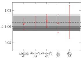
Figure 1: (Color online) Estimates of the critical exponent $\nu$ of the 2D Ising model from the FSS of the indicated observables. The horizontal lines indicate the plain average $\bar{\nu}_{\mathrm{plain}}$ (dotted), the error-weighted mean $\bar{\nu}_{\mathrm{err}}$ (dashed), and the covariance-weighted mean $\bar{\nu}_{\mathrm{cov}}$ (solid). The shaded areas indicate the corresponding one-sigma environments $\bar{\nu}\pm\sigma_{\mathrm{corr}}$.

Similar considerations apply to the correlations between estimates of different exponents. In particular, taking the scaling relations for critical exponents into account, the magnetic and energetic scaling dimensions might be estimated from different observables. For instance, the magnetic scaling dimension can be estimated via the relations $x_{\sigma}=\beta/\nu$ and $x_{\sigma}=d/2-\gamma/2\nu$ from the FSS of the magnetization at its inflection point and the magnetic susceptibility at its maximum via the relations $\langle|m|\rangle_{\mathrm{inf}}(L)=m_{0}L^{-\beta/\nu}$ and $\chi_{\mathrm{max}}(L)=\chi_{0}L^{\gamma/\nu}$, respectively. Table 3 summarizes the correlation analysis for $x_{\sigma}$ in the 2D model, where through the pronounced anti-correlation of the two estimates of $x_{\sigma}$ the uncorrelated error $\sigma_{\mathrm{uncorr}}$ over-estimates statistical fluctuations, and already the error-weighted mean is somewhat more precise than either of the two single estimates. Still, the covariance-weighted mean is even more precise, yielding $\bar{x}_{\sigma,\mathrm{cov}}=0.125(1)$, directly at the exact value $x_{\sigma}=1/8$. For the 3D model, on the other hand, (only) the correlation analysis reveals that both estimates of $x_{\sigma}$ are nearly uncorrelated such that, for this specific case, the full result approximately coincides with the naive approach neglecting correlations.

To summarize, we have seen that substantial cross-correlations exist between quantities estimated via histogram analyses from time series of Markov chain MC simulations. Taking these into account by a straightforward extension of the common data analysis reveals a generic underestimation of statistical error by the conventional approach. On the other hand, it suggests improved estimators with often substantially reduced statistical fluctuation resulting, for some examples, in a threefold reduction of statistical error which could otherwise only be achieved with an about tenfold increase of simulation time with the conventional analysis. While these effects have been illustrated here for the case of the critical exponents of the Ising model, very similar behavior is expected for non-universal quantities, including properties of first-order transitions Janke (2003), and for different applications, including the problems in soft-matter systems Holm and Kremer (2005), for quantum critical points Vojta (2003), or the extremely costly simulations of disordered systems Holovatch (2007). These applications, together with the flexibility in choosing different thermal or FSS approaches, render the outlined technique quite generic.

Table 3: Correlation analysis and averages of estimates of the magnetic scaling dimension $x_{\sigma}$ of the 2D Ising model from the scaling of the magnetization at its inflection point and the magnetic susceptibility at its maximum.

		fits		corr. coeff./weights
		$x_{\sigma}$	$\sigma$	$\displaystyle\langle|m|\rangle_{\mathrm{inf}}$	$\displaystyle\chi_{\mathrm{max}}$
$\displaystyle\langle|m|\rangle_{\mathrm{inf}}$		$0.1167$	$0.0054$	$1.0000$	$-0.6414$
$\displaystyle\chi_{\mathrm{max}}$		$0.1271$	$0.0020$	$-0.6414$	$1.0000$
$\bar{x}_{\mathrm{plain}}$	$\sigma_{\mathrm{uncorr}}$	$0.1219$	$0.0027$	$1.0000$	$1.0000$
	$\sigma_{\mathrm{corr}}$		$0.0021$
$\bar{x}_{\mathrm{err}}$	$\sigma_{\mathrm{uncorr}}$	$0.1261$	$0.0016$	$0.0944$	$0.9056$
	$\sigma_{\mathrm{corr}}$		$0.0013$
$\bar{x}_{\mathrm{cov}}$	$\sigma_{\mathrm{corr}}$	$0.1250$	$0.0010$	$0.2050$	$0.7950$
reference value		$0.125$

M.W. acknowledges support by the DFG through the Emmy Noether Programme under contract No. WE4425/1-1.

References

- Chaikin and Lubensky (2000) P. M. Chaikin and T. C. Lubensky, Principles of Condensed Matter Physics (Cambridge University Press, Cambridge, 2000).
- Bergström and Goobar (2004) L. Bergström and A. Goobar, Cosmology and Particle Astrophysics (Springer, Berlin, 2004).
- Vojta (2003) M. Vojta, Rep. Prog. Phys. 66, 2069 (2003).
- Binder and Landau (2005) K. Binder and D. P. Landau, A Guide to Monte Carlo Simulations in Statistical Physics (Cambridge University Press, Cambridge, 2005), 2nd ed.
- Pelissetto and Vicari (2002) A. Pelissetto and E. Vicari, Phys. Rep. 368, 549 (2002).
- Janke (2003) W. Janke, in Computer Simulations of Surfaces and Interfaces, edited by B. Dünweg, D. P. Landau, and A. I. Milchev (Kluwer, Dordrecht, 2003), vol. 114 of NATO Science Series, II. Mathematics, Physics and Chemistry, p. 111.
- Ferrenberg and Swendsen (1988) A. M. Ferrenberg and R. H. Swendsen, Phys. Rev. Lett. 61, 2635 (1988); 63, 1195 (1989).
- Berg and Neuhaus (1992) B. A. Berg and T. Neuhaus, Phys. Rev. Lett. 68, 9 (1992).
- Efron and Tibshirani (1998) B. Efron and R. J. Tibshirani, An Introduction to the Bootstrap (Chapman and Hall, Boca Raton, 1998).
- Berg (2004) B. A. Berg, Markov Chain Monte Carlo Simulations and Their Statistical Analysis (World Scientific, Singapore, 2004).
- Ferrenberg and Landau (1991) A. M. Ferrenberg and D. P. Landau, Phys. Rev. B 44, 5081 (1991).
- Ballesteros et al. (1996) H. G. Ballesteros, L. A. Fernández, V. Martín-Mayor, and A. Muñoz Sudupe, Phys. Lett. B 378, 207 (1996).
- Hasenbusch (1999) M. Hasenbusch, J. Phys. A 32, 4851 (1999).
- Brandt (1998) S. Brandt, Data Analysis: Statistical and Computational Methods for Scientists and Engineers (Springer, Berlin, 1998), 3rd ed.
- Janke and Sauer (1997) W. Janke and T. Sauer, J. Chem. Phys. 107, 5821 (1997).
- Michael (1994) C. Michael, Phys. Rev. D 49, 2616 (1994).
- Blöte et al. (1999) H. W. J. Blöte, L. N. Shchur, and A. L. Talapov, Int. J. Mod. Phys. C 10, 1137 (1999).
- Holm and Kremer (2005) C. Holm and K. Kremer, eds., Advanced Computer Simulation Approaches for Soft Matter Sciences, vol. 1 and 2 (Springer, Berlin, 2005).
- Holovatch (2007) Y. Holovatch, ed., Order, Disorder and Criticality, vol. 1 and 2 (World Scientific, Singapore, 2007).