Pattern formation in systems with competing interactions

Abstract

There is a growing interest, inspired by advances in technology, in the low temperature physics of thin films. These quasi-2D systems show a wide range of ordering effects including formation of striped states, reorientation transitions, bubble formation in strong magnetic fields, etc. The origins of these phenomena are, in many cases, traced to competition between short ranged exchange ferromagnetic interactions, favoring a homogeneous ordered state, and the long ranged dipole-dipole interaction, which opposes such ordering on the scale of the whole sample. The present theoretical understanding of these phenomena is based on a combination of variational methods and a variety of approximations, e.g., mean-field and spin-wave theory. The comparison between the predictions of these approximate methods and the results of MonteCarlo simulations are often difficult because of the slow relaxation dynamics associated with the long-range nature of the dipole-dipole interactions. In this note we will review recent work where we prove existence of periodic structures in some lattice and continuum model systems with competing interactions. The continuum models have also been used to describe micromagnets, diblock polymers, etc.

1 Introduction

The formation of mesoscopic (nano/micro) scale patterns (interpreted broadly) in equilibrium systems is often due to a competition between interactions favoring different microscopic structures. As an example suppose we begin with a short ranged potential favoring local “alignment” of the microscopic constituents of the system, e.g. nearest neighbor ferromagnetic interactions of an Ising spin system. At low temperature this would lead to essentially all spins pointing in the same direction. If we now add a long range interaction which does not like this ordering then the system will do the best it can by forming mesoscopic domains with different aligments.

Such a competition occurs in many systems. It is well illustrated in patterns observed in the low temperature structure of thin films. These quasi-2D systems show a wide range of ordering effects including formation of striped states, reorientation transitions, etc. DMW00 ; Seul and Wolfe (1992), see Figure 1.

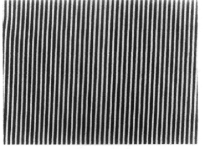
Figure 1: Ferrimagnetic garnet film on GGG at zero magnetic field and $T=0.6$$T_{c}$, with $T_{c}=192^{\circ}C$. From M. Seul and R. Wolfe, PRA (1992)

The origins of these phenomena can, in many cases, be traced to the competition between short ranged exchange (ferromagnetic) interactions, favoring a homogeneous ordered state, and long ranged dipole-dipole type interactions, which oppose such ordering on the scale of the whole sample DMW00 ; Seul and Wolfe (1992); TKNV05 ; Spivak and Kivelson (2006).

This type of competitive interaction is believed responsible for many of the observed patterns in a great variety of systems, including thin magnetic films Seul and Wolfe (1992), micromagnets Brazovskii (1975); DKMO ; Garel and Doniach (1982), diblock copolymers Hohenberg and Swift (1995); Leibler (1980); Ohta and Kawasaki (1986), anisotropic electron gases Spivak and Kivelson (2004, 2006), Langmuir monolayers Mohwald (1988), lipid monolayers Keller and McConnell (1999), liquid crystals Maclennan and Seul (1992), polymer films Harrison et al. (2000), polyelectrolytes Borue and Erukhimovich (1988), charge-density waves in layered transition metals McMillian (1975), superconducting films Emery and Kivelson (1993), colloidal suspensions and cell membranes Destainville1 ; Destainville2 . Many of these systems are characterized by low temperature phases displaying periodic mesoscopic patterns, such as stripes or bubbles.

The simplest models to describe such systems are Ising or “soft spin” models with a short range ferromagnetic interaction and a power law long range antiferromagnetic pair potential MacIsaac et al. (1995); Arlett et al. (1996); Stoycheva and Singer (1999); Low et al. (1994); Grousson et al. (2000); Garel and Doniach (1982); Chayes et al. (1996). The zero temperature phase diagram of these models has been thoroughly investigated over the last decade and a sequence of transitions from an antiferromagnetic homogeneous state to periodic striped or lamellar phases with domains of increasing sizes has been predicted, as the strength of the ferromagnetic coupling is increased from zero to large positive values. These theoretical predictions are mostly based on a combination of variational techniques and stability analysis: they start by assuming a periodic structure, proceed by computing the corresponding energy and finally by comparing that energy to the energy of other candidate structures, usually by a combination of analytical and numerical tools. These calculations give an excellent account of some of the observed “universal” patterns displayed by the aforementioned systems. However they run the risk of overlooking complex microphases that have not been previously identified Bates and Fredrickson (1999). This risk is particularly significant in cases, as those under analysis, where dynamically (e.g. in Monte Carlo simulations) the domain walls separating different microphases are very long lived as the temperature is lowered MacIsaac et al. (1995).

To develop a complete ab initio theory of pattern formations it is necessary to be able to first prove periodicity of the ground state and then proceed with a variational computation within the given ansatz. The problem is not simple. Most of the mathematically rigorous techniques developed for obtaining the low temperature phase diagram of spin systems, e.g., the Pirogov–Sinai theory Pirogov and Sinai (1975), depend on the interaction being short range. Only methods based on reflection positivity Frohlich et al. (1978) or on convexity Hubbard (1978); Pokrovsky and Uimin (1978); Jedrzejewski and Miekisz (2000a, b); Kerimov (1999) seem applicable to the kind of potentials considered here.

In this paper we review recent progress on the construction of periodic ground states in one and two dimensional spin systems, both in the case of discrete and continuum systems GLL1 ; GLL2 ; GLL3 . The analysis is based on reflection positivity methods Frohlich et al. (1978). In the cases where it applies, it gives a full justification of the variational calculations based on the periodicity assumption.

The paper is organized as follows: in the next section we describe the class of discrete and continuum spin models we will be concerned with; next, we present our main results about the zero temperature phase diagram of these models; then we give a sketch of the proof and, finally, we draw our conclusions.

2 The models

2.1 Discrete models

The simplest discrete spin model describing the class of systems we are interested in is an Ising model with the following Hamiltonian:

$$H^{(1)}_{\Lambda}=-J\sum_{<{\bf x},{\bf y}>}\sigma_{\bf x}\sigma_{\bf y}+K\sum_{{\bf x}\neq{\bf y}}\frac{\sigma_{\bf x}\sigma_{\bf y}}{|{\bf x}-{\bf y}|^{p}}\;,$$ (1)

where: $\Lambda\subset\hbox{\msytw Z}^{d}$ is a $d$-dimensional cubic box with (say) open boundary conditions; the first summation is over all pairs of nearest neighbor sites in $\Lambda$, while the second summation is over pairs of distinct sites of $\Lambda$; if ${\bf x}\in\Lambda$, $\sigma_{\bf x}\in\{\pm 1\}$ is the Ising spin variable; $p>d$, in order to guarantee the summability of the long range potential. A physically interesting case is the one corresponding to $d=2$ and $p=3$, in which case the long range term mimics the effect of the 3D dipolar interactions among out-of-plane magnetic moments constrained to a two–dimensional surface as in a thin magnetic film.

The ground states of (1) are well understood in two limiting cases: if $K=0$, the ground state is ferromagnetic, consisting of spins all aligned either up or down; if $J=0$, then the ground state is antiferromagnetic, displaying Néel order of period 2. For general $J$ and $K$ the ground state is not known. A variational calculation supports the conjecture that in $d=2$, $p=3$, the ground state is periodic and striped for all $J,K>0$ with $J/K$ larger than a critical value $j_{0}$. In particular, it is remarkable that the checkerboard state has higher energy than the striped one.

Another natural class of discrete spin models is described by the following Hamiltonian:

$$H^{(2)}_{\Lambda}=-J\sum_{\langle{\bf x},{\bf y}\rangle}\vec{S}_{{\bf x}}\cdot\vec{S}_{{\bf y}}+K\sum_{{\bf x}\neq{\bf y}}\vec{S}_{\bf x}\hat{W}^{dip}({\bf x}-{\bf y})\vec{S}_{{\bf y}}\;,$$ (2)

where $\vec{S}$ are classical Heisenberg spins and

$$W^{dip}_{ij}({\bf x})=-\partial_{i}\partial_{j}\frac{1}{|{\bf x}|}=\frac{1}{|{\bf x}|^{3}}\Big{(}\delta_{ij}-3\frac{x_{i}x_{j}}{|x|^{2}}\Big{)}\;.$$ (3)

Also in this case, in the limiting cases $J=0$ or $K=0$ the ground state can be determined exactly: it is ferromagnetic if $K=0$; it displays an in-plane uniaxial AF order and is continuously degenerate if $J=0$. In the general case the ground state is unknown.

On the mathematical side, the problem of proving periodicity is very difficult GLL1 ; GLL2 ; GLL3 ; Mueller (1993); CO . There are very few models where one can demonstrate rigorously that energy minimizers are periodic. Note that the problem is not trivial already in 1D.

2.2 Continuum models

It is sometimes convenient to consider effective continuum descriptions of the same spin system. If $\sigma(x)$ $\in\{\pm 1\}$ and $X_{+}$ is the region where $\sigma(x)=+$, one can consider the following model:

$$H^{(3)}_{\Lambda}=2J|\partial X_{+}|+K\int_{\Lambda\times\Lambda}d{\bf x}d{\bf y}\frac{\sigma(x)\sigma(y)}{|x-y|^{p}+a}\;,\qquad p>d\;.$$ (4)

The case of “soft” local magnetization $\phi(x)\in\hbox{\msytw R}$ is often considered, too:

$$H^{(4)}_{\Lambda}=\int_{\Lambda}dx\Big{[}|\nabla\phi|^{2}+F(\phi(x))\Big{]}+K\int_{\Lambda\times\Lambda}d{\bf x}d{\bf y}\frac{\phi(x)\phi(y)}{|x-y|^{p}+a}\;.$$ (5)

In the two equations above $a>0$ is an ultraviolet regulator, playing the role of the lattice spacing in the previous discrete model. In the case of the soft spin model, $F$ is a symmetric double well potential, with two minima located at $\phi=\pm\phi_{0}\neq 0$: typical examples to keep in mind are $F(\phi)=(\phi^{2}-\phi_{0}^{2})^{2}$ or $F(\phi)=(|\phi|-|\phi_{0}|)^{2}$ or

$$F(\phi)=\left\{\matrix{-\frac{\phi^{2}}{2}-\frac{1}{\beta}I(\phi)\,,\hskip 28.45274pt{\rm if}\ |\phi|<1\,,\cr+\infty\;,\hfill\hskip 34.14322pt{\rm if}\ |\phi|\geq 1\;,\cr}\right.\qquad$$ (6)

where $I(\phi)=-\frac{1-\phi}{2}\log\frac{1-\phi}{2}-\frac{1+\phi}{2}\log\frac{1+\phi}{2}$. The gradient term in (5) represents the cost of a transition between two phases (the homogeneous magnetized phases induced by the short range exchange interaction), while the term $F$ represents the local free energy density of a homogeneous system in a mean field approximation.

Similarly to the discrete case, the minimizers of (4) and (5) can be easily determined in the limiting cases where only the attractive or only the repulsive interactions are present. In the presence of a competition, it is again conjectured, on the basis of variational computations, that the minimizers are periodic and that they display periodic striped (or lamellar) order Spivak and Kivelson (2004).

Both the models in this and in the previous section can be extended to the case of non zero magnetic field, in which case the expected phase diagram is even more complex, e.g., periodic bubbled states are expected at high enough magnetic field Garel and Doniach (1982). The rigorous results concerning these more complicated cases are still very partial, and we will not consider them explictly in this paper.

3 Main results

We have proven a number of results in the 1D case, both for the discrete and the continuum models. The higher dimensional case is in many respects still open. Partial results include an example of a 2D dipole system with in-plane dipoles, reminiscent of model (2), that, in the presence of a special nearest neighbor ferromagentic interaction, has periodic ground states displaying striped periodic order. In the following we want to describe these results, starting from the case of one dimension.

3.1 One dimension

In one spatial dimension, we have a quite complete picture of the ground states of models $H^{(1)}_{\Lambda}$, $H^{(3)}_{\Lambda}$ and $H^{(4)}_{\Lambda}$. Regarding the models with Hamiltonian $H^{(1)}_{\Lambda}$ and $H^{(3)}_{\Lambda}$, our main result can be summarized as follows GLL1 .

Theorem 1. Let $d=1$. For any $J,K\geq 0$ and any $p>1$, the specific ground state energies $E_{0}^{(1)}(\Lambda)$ and $E^{(3)}(\Lambda)$ of, respectively, $H_{\Lambda}^{(1)}$ and $H^{(3)}_{\Lambda}$ in the thermodynamic limit are given by:

$$\lim_{|\Lambda|\rightarrow\infty}\frac{1}{|\Lambda|}E_{0}^{(1)}(\Lambda)=\inf_{h\in\hbox{\msytw N}}e_{1}(h)\;,$$

$$\lim_{|\Lambda|\rightarrow\infty}\frac{1}{|\Lambda|}E_{0}^{(3)}(\Lambda)=\inf_{h\in\hbox{\msytw R}_{+}}e_{3}(h)\;,$$ (7)

where $e_{1}(h)$ and $e_{3}(h)$ are the specific energies of a striped periodic configuration of period $2h$, obtained by extending periodically over the whole line the functions $\sigma_{x}={\rm sgn}(x)$, $x=-h+1,\ldots,h$, and $\sigma(x)={\rm sgn}(x)$, $x\in(-h,h]$, respectively. In the presence of periodic boundary conditions, the only ground states of $H^{(3)}_{\Lambda}$ are the optimal periodic striped configurations; in the case of the discrete Ising model, the same conclusion is valid, if the ring has a length divisible by the optimal period.

Remarks.
1) The optimal period $2h$ increases with $J$; when $J=0$, $h=1$ in the discrete and $h=0$ in the continuum, i.e., as $J\to 0$ the oscillations become wild and the period shrinks to zero. Depending on the values of $p$, $J$ and $K$, the ground state has finite periodicity or is ferromagnetic: if $p>2$ and $J/K$ smaller than a suitable $j_{c}$ the period is finite and diverges at $j_{c}$; if $J/K\geq j_{c}$ the ground state is FM. If $1<p\leq 2$, then $j_{c}=\infty$ and the period will increase as $J/K$ increases, becoming mesoscopic/macroscopic.
2) The proofs are based on a generalized notion of reflection positivity (RP), see Frohlich et al. (1978) and below for the description of reflection positivity. In the present case one needs first to describe the states as collections of blocks, and then apply RP to the effective model of interacting blocks.
3) The proof works equally well for a larger class of long range potentials $v(r)$: it is enough that $v(r)$ is the Laplace transform of a positive measure, i.e., $v(r)=\int_{0}^{\infty}d\alpha\,\mu(\alpha)e^{-\alpha|r|}$. This class of interactions include, besides the power laws, the exponentials and arbitrary positive linear combinations of exponentials.
4) Inclusion of temperature is not trivial: block RP is lost for $\beta<+\infty$. One expects for $p>1$ a unique Gibbs measure, whose typical configurations are close to the periodic ground states determined above. This is “easy” to prove for $J=0$ and $p>2$ and is probably not true for $p<1$ when the potential is not absolutely summable. (Note: for purely ferromagnetic power law potentials $v(r)\sim-1/r^{p}$, there is a finite temperature spontaneous magnetization for $1<p\leq 2$).
5) As mentioned above, we are unable at present to extend our results to the case where there is a magnetic field acting on the system or there is a non zero specified magnetization. This is true both for the lattice, where very complex structures are expected (e.g., for $J=0$ the existence of a “devil’s staircase” has been proved PerBak ), and for the continuum where one expects simple periodic structures with blocks of alternate lengths Huse08 .

The proof of Theorem 1 works exactly in the same way both for $H_{\Lambda}^{(1)}$ and for $H_{\Lambda}^{(3)}$. The extension to $H_{\Lambda}^{(4)}$ requires a refinement of the block RP ideas, see GLL3 . The final result, stated in an informal way, is the following (see GLL3 for a mathematically rigorous statement, making precise the choice of boundary conditions and the notion of infinite volume minimizers).

Theorem 2. If $d=1$, all the minimizers of $H_{\Lambda}^{(4)}$ are either simply periodic, of finite period $T$, with zero average, or of constant sign (and are constant if $F$ is convex on $\hbox{\msytw R}^{+}$). By “simply periodic” we mean that within a period the minimizer has only one positive and one negative region, with the negative part obtained by a reflection from the positive part.

Remarks.
1) Similarly to the “hard” spin case, the proof works even if the power law potential is replaced by a $v(r)$ that is the Laplace transform of a positive measure, in particular in the case of an exponential interaction. Of course, as in Theorem 1, the value of the period and, in this case, the shape of the minimizer within one period, is obtained by a variational computation, whose result depends on $v(r)$, $J$ and $K$.
2) One can provide explicit examples of cases where the system displays a transition from a homogeneous to a periodic non homogeneous state. For instance, if $F(\phi)=(|\phi|-1)^{2}$ and $v(x)=\lambda e^{-|x|}$, the previous result combined with an explicit computation imply that the minimizer is constant for $\lambda\leq 3/2$ and periodic with zero average for $\lambda>3/2$.
3) The result of Theorem 2 can be extended to a larger class of free energy functionals. In particular, it can be applied to the study of effective 1D models for martensitic phase transitions, see Kohn and Mueller. (1992); Mueller (1993).

3.2 Two dimensions

As mentioned above, the case of two or more dimensions is in many respects still open. Partial results include:
1) lower bounds on the specific ground state energy of (1) and (4), agreeing at lowest order with the energy of the striped case;
2) an example of a 2D dipole system with in-plane dipoles and a special exchange interaction, whose ground states can be proved to be striped and periodic.

For the precise statement and the proof of claim (1), we refer to GLL1 (let us just mention that the proof is based on apriori bounds on the energy of Peierls contours). Here we want to describe in more detail the result mentioned in item (2), which is, as far as we know, the only example of a spin model in two or more dimensions with real dipole interactions, for which existence of periodic striped order has been proved.

The two dimensional spin model that we consider is a modification of model $H^{(2)}_{\Lambda}$, defined by the following Hamiltonian:

$$\widetilde{H}^{(2)}_{\Lambda}=\sum_{{\bf x}\neq{\bf y}}\vec{S}_{\bf x}\hat{W}^{dip}({\bf x}-{\bf y})\vec{S}_{\bf y}-\sum_{\langle{\bf x},{\bf y}\rangle}\Big{(}J\vec{S}_{x}\cdot\vec{S}_{y}+\lambda(\vec{S}_{x}\cdot\vec{S}_{y})^{2}\Big{)}\;,$$ (8)

where $\Lambda$ is a 2D square lattice, $\lambda\geq 0$ and $\vec{S}_{\bf x}$ are in-plane spins, whose allowed directions are only $\uparrow$, $\downarrow$, $\rightarrow$ and $\leftarrow$. Note that the $\lambda$ term has the effect of encouraging alignment or antialignment but this term alone cannot create periodic order. Our main result can be summarized as follows.

Theorem 3. Let $d=2$. For $J\geq 0$ and $\lambda$ large enough, the specific ground state energy of $\widetilde{H}^{(2)}_{\lambda}$ in the thermodynamic limit is given by:

$$\lim_{|\Lambda|\rightarrow\infty}\frac{1}{|\Lambda|}\widetilde{E}^{(2)}_{0}(\Lambda)=\min_{h\in\hbox{\msytw Z}+}\tilde{e}_{2}(h)\;,$$ (9)

where $\tilde{e}_{2}(h)$ is the specific energy of a striped configuration of period $2h$, consisting of stripes of uniformly polarized columns, all of size $h$, and with alternate up/down polarization. On a torus of side divisible by the optimal period, the only ground states are the optimal periodic striped configurations, either displaced vertically or horizontally.

Remarks.
1) The condition on $\lambda$ is not uniform in $J$. It is unclear whether the same result should be valid for large $\lambda$, uniformly in $J$, or even up to $\lambda=0$.
2) The proof of Theorem 3 is based on an extension of the ideas of the proof of Theorem 1. We first show that, for $\lambda=+\infty$, the system preferes to have the columns all completely polarized (because of the anisotropy of the dipolar potential); this means that, for the purpose of computing the ground state energy, we can restrict to 1D confirgurations of up or down columns, and at this point we can apply Theorem 1. Next we show that if $\lambda$ is sufficiently large, then in the ground state there are no perpendicular neighboring spins, and this concludes the proof. See GLL2 for details.

4 Reflection positivity

As mentioned in previous sections, the proofs of Theorem 2 and 3 extend the ideas of the proof of Theorem 1, which is based on a generalized notion of reflection positivity. Let us clarify here what we mean by reflection positivity, and how can one apply it to the problem of determining the ground state of $H^{(1)}_{\Lambda}$, at least in the simple case $J=0$.

Let us consider the Hamiltonian

$$H_{\Lambda}=\sum_{-N<x<y\leq N}\sigma_{x}\sigma_{y}\,v(y-x)\;,$$ (10)

in the presence of periodic boundary conditions and with $v(x)=\sum_{n\in\hbox{\msytw Z}}|x+2nN|^{-p}$. Note that, if $x>0$, using that $x^{-p}=\Gamma(p)^{-1}\int_{0}^{\infty}d\alpha\alpha^{p-1}e^{-\alpha x}$, we can rewrite:

$$v(x)=\int_{0}^{\infty}\frac{d\alpha}{\Gamma(p)}\frac{\alpha^{p-1}}{1-e^{-2\alpha N}}(e^{-\alpha x}+e^{-\alpha(2N-x)})\;.$$ (11)

Therefore,

$$H_{\Lambda}(\underline{\sigma})=H_{L}(\underline{\sigma})+H_{R}(\underline{\sigma})+\sum_{x=-N+1}^{0}\sum_{y=1}^{N}\int_{0}^{\infty}d\alpha\,\mu(\alpha)\sigma_{x}\sigma_{y}\,(e^{-\alpha(y-x)}+e^{-\alpha(2N-y+x)})\;,$$ (12)

where: $\mu(\alpha)=\frac{1}{\Gamma(p)}\frac{\alpha^{p-1}}{1-e^{-2\alpha N}}$, $\underline{\sigma}=(\sigma_{-N+1},\ldots,\sigma_{-1},\sigma_{0},\ldots,\sigma_{N})$ and

$$H_{L}(\underline{\sigma})=\sum_{-N<x<x^{\prime}<0}\sigma_{x}\sigma_{x^{\prime}}\,v(x^{\prime}-x)\;,$$

$$H_{R}(\underline{\sigma})=\sum_{0\leq y<y^{\prime}\leq N}\sigma_{y}\sigma_{y^{\prime}}\,v(y^{\prime}-y)\;.$$ (13)

If $\theta\underline{\sigma}$ is the configuration with $(\theta\underline{\sigma})_{i}=-\sigma_{-i+1}$ and $A_{\alpha}(\underline{\sigma})$ is defined as

$$A_{\alpha}(\underline{\sigma})=\sum_{y=0}^{N}\sigma_{y}e^{-\alpha y}\;,$$ (14)

we can rewrite (12) in the form:

$$H_{\Lambda}(\underline{\sigma})=H_{L}(\underline{\sigma})+H_{R}(\underline{\sigma})-\int_{0}^{\infty}d\alpha\mu(\alpha)e^{\alpha}\big{[}A_{\alpha}(\underline{\sigma})A_{\alpha}(\theta\underline{\sigma})+e^{-2\alpha N}A_{-\alpha}(\underline{\sigma})A_{-\alpha}(\theta\underline{\sigma})\big{]}\;,$$ (15)

Now the crucial remark is that the integral in the right hand side of (15) defines a scalar product between the configurations $\underline{\sigma}$ and $\theta\underline{\sigma}$. Therefore, defining

$$\langle{\underline{\sigma}_{1},\underline{\sigma}_{2}}\rangle=\int_{0}^{\infty}d\alpha\,\mu(\alpha)e^{\alpha}\big{[}A_{\alpha}(\underline{\sigma}_{1})A_{\alpha}(\underline{\sigma}_{2})+e^{-2\alpha N}A_{-\alpha}(\underline{\sigma}_{1})A_{-\alpha}(\underline{\sigma}_{2})\big{]}$$ (16)

and using that, for any scalar product,

$$\langle{\underline{\sigma}_{1},\underline{\sigma}_{2}}\rangle\leq\frac{1}{2}\Big{(}\langle{\underline{\sigma}_{1},\underline{\sigma}_{1}}\rangle+\langle{\underline{\sigma}_{2},\underline{\sigma}_{2}}\rangle\Big{)}\;,$$ (17)

we get

$$H_{\Lambda}(\underline{\sigma})\geq\frac{1}{2}\Big{(}H_{L}(\underline{\sigma})-\langle{\theta\underline{\sigma},\theta\underline{\sigma}}\rangle+H_{R}(\theta\underline{\sigma})\Big{)}+\frac{1}{2}\Big{(}H_{L}(\theta\underline{\sigma})-\langle{\underline{\sigma},\underline{\sigma}}\rangle+H_{R}(\underline{\sigma})\Big{)}\;,$$ (18)

which means

$$H_{\Lambda}(\underline{\sigma})\geq\frac{1}{2}\big{(}H_{\Lambda}(\underline{\sigma}_{L})+H_{\Lambda}(\underline{\sigma}_{R})\big{)}\;,$$ (19)

with $\underline{\sigma}_{L}=(\sigma_{-N+1},\ldots,\sigma_{0},-\sigma_{0},\ldots,\-\sigma_{-N+1})$ and $\underline{\sigma}_{R}=(-\sigma_{N},\ldots,-\sigma_{1},\sigma_{1},\ldots,\sigma_{N})$. In other words, given any configuration $\underline{\sigma}$, at least one of the two configurations obtained from $\underline{\sigma}$ by reflection around $(0,1)$ has better (or equal) energy than the original configuration. So, if we want to reduce the energy, we can keep reflecting about all possible bonds; proceeding like this we end up with the configuration $\cdots+-+-+-\cdots$

In the presence of a nearest neighbor ferromagnetic interaction, we proceed in a similar fation, but we only reflect about the bonds separating a plus from a minus spin. After repeated refelctions we are left with a configuration consisting of a sequence of blocks of polarized spins, all of the same size and with alternate polarization. For more details, see GLL1 (see also GLL2 and GLL3 for a corrected discussion about the checkerboard estimate).

5 Conclusions

In this note we reviewed some recent rigorous results about existence of periodic striped states for a number of 1D and 2D spin systems, described by discrete or continuum models. The proofs are based on a generalized notion of reflection positivity, and require the long range interaction to be reflection positive, i.e., the Laplace transform of a positive measure. The short range interaction needs to be among nearest neighbor sites. The proof applies to 1D systems or higher dimensional systems which can be proven to display 1D ground states by apriori energy estimates. Open problems include the inclusion of magnetic fields, of a non zero temperature and, most importantly, the proof that the ground states of the $d$–dimensional spin systems described by Eqs. (1), (2), (4) and (5) are translational invariant in $d-1$ coordinate directions. So far, this claim has only been proven for $\widetilde{H}_{\Lambda}^{(2)}$ in (8). There are good hopes to extend the proof to a new class of 2D models, relevant for the description of martensitic phase transitions Kohn and Mueller. (1992).

Let us also mention that these models with competing interactions are closely related to a class of systems considered by Lebowitz and Penrose in LP . They considered the case when the pair potential is the sum of a short range interaction, $\phi(r)$, favoring phase segregation on the macroscopic scale and a long range (Kac type) interaction favoring a uniform density, e.g. $v_{\gamma}(r)=\alpha\gamma^{d}\exp\{-\gamma r\},\alpha>0$, $d$ the space dimension. Lebowitz and Penrose proved that, in the limit $\gamma\rightarrow 0$, this competition will result in the system breaking up into a “foam” consisting of mesoscopic regions of the different phases. These will have a characteristic length large compared to that of the short range potential and small compared to that of the long range potential $\gamma^{-1}$. This may give rise to the different kinds of patterns observed experimentally in many systems. We have shown in GLL2 that in one dimension when the long range Kac potential is of the exponential type, or more generally is reflection-positive, then these droplets will form a periodic ground states with period of order $\gamma^{-2/3}$. A heuristic argument suggests that the scaling of the patterns in three dimensions will be like $\gamma^{-4/5}$ SF03 .

As pointed out in SF03 the effect of the long range repulsive interaction is similar to that of surfactants which lower the surface tension between the two phases. We plan to explore further the general phenomena of pattern formation due to competing interactions which occurs in many systems beyond those described earlier, e.g. Langmuir monolayers, lipid monolayers, liquid crystals, two dimensional electron gases, diblock copolymers, etc. This type of competition may also be responsible for some of the phenomona observed in confined water 38 and in aqueous surfactant solutions 39 . A related kind of competition, due to geometric frustration, can induce the formation of striped periodic patterns in buckled collodial monolayers 40 . As pointed out in 40 ; SL08 , this is related to stripe formation in compressible antiferromagnents on a triangular lattice 41 .

References

- Arlett et al. (1996) J. Arlett, J. P. Whitehead, A. B. MacIsaac, and K. De’Bell, Phys. Rev. B 54, 3394 (1996).
- (2) P. Bak and R. Bruinsma, Phys. Rev. Lett. 49, 249–251 (1982).
- Ball (2001) P. Ball, The self–made tapestry: pattern formation in nature (Oxford Univ. Press, 2001).
- Bates and Fredrickson (1999) F. S. Bates and G. H. Fredrickson, Physics Today 52-2, 32 (1999).
- Borue and Erukhimovich (1988) V. Y. Borue and I. Y. Erukhimovich, Macromolecules 21, 3240 (1988).
- Bowman and Newell (1998) C. Bowman and A. C. Newell, Rev. Mod. Phys. 70, 289 (1998).
- Brazovskii (1975) S. A. Brazovskii, Zh. Eksp. Teor. Fiz. 68, 175 (1975).
- Chayes et al. (1996) L. Chayes, V. Emery, S. Kivelson, Z. Nussinov, and G. Tarjus, Phys. A 225, 129 (1996).
- (9) X. Chen and Y. Oshita, SIAM J. Math. Anal. 37, 1299-1332 (2005).
- (10) A. DeSimone, R. V. Kohn, F. Otto and S. Müller, in The Science of Hysteresis II: Physical Modeling, Micromagnetics, and Magnetization Dynamics, G. Bertotti and I. Mayergoyz eds., pp. 269–381, Elsevier (2001).
- (11) K. De’Bell, A.B. Mac Issac and J.P. Whitehead, Rev. Mod. Phys. 72, 225 (2000).
- (12) N. Destainville, Phys. Rev. E 77, 011905 (2008).
- (13) N. Destainville and L. Foret, Phys. Rev. E 77, 051403 (2008).
- Emery and Kivelson (1993) V. J. Emery and S. A. Kivelson, Physica C 209, 597 (1993).
- Frohlich et al. (1978) J. Frohlich, R. Israel, E. Lieb, and B. Simon, Comm. Math. Phys. 62, 1 (1978).
- Garel and Doniach (1982) T. Garel and S. Doniach, Phys. Rev. B 26, 325 (1982).
- (17) A. Giuliani, J. L. Lebowitz and E. H. Lieb, Phys. Rev. B 74, 064420 (2006).
- (18) A. Giuliani, J. L. Lebowitz and E. H. Lieb, Phys. Rev. B 76, 184426 (2007).
- (19) A. Giuliani, J. L. Lebowitz and E. H. Lieb, Comm. Math. Phys. 286, 163–177 (2009).
- Grousson et al. (2000) M. Grousson, G. Tarjus, and P. Viot, Phys. Rev. E 62, 7781 (2000).
- (21) L. Gu, B. Chakraborty, P.L. Garrido, M. Phane and J.L. Lebowitz, Phys. Rev. B 53, 11985 (1996).
- (22) Y. Han, Y. Shokef, A.M. Alsayed, P. Yunker, T.C. Lubensky, A.G. Yodh, Nature 456, 898–903 (2008).
- Harrison et al. (2000) C. Harrison, D. H. Adamson, Z. Cheng, J. M. Sebastian, S. Sethuraman, D. A. Huse, R. A. Register, and P. M. Chaikin, Science 290, 1558 (2000).
- Hohenberg and Swift (1995) P. C. Hohenberg and J. B. Swift, Phys. Rev. E 52, 1828 (1995).
- Hubbard (1978) J. Hubbard, Phys. Rev. B 17, 494 (1978).
- Jedrzejewski and Miekisz (2000a) J. Jedrzejewski and J. Miekisz, Europhys. Lett. 50, 307 (2000a).
- Jedrzejewski and Miekisz (2000b) J. Jedrzejewski and J. Miekisz, Jour. Stat. Phys. 98, 589 (2000b).
- Keller and McConnell (1999) S. L. Keller and H. M. McConnell, Phys. Rev. Lett. 82, 1602 (1999).
- Kerimov (1999) A. Kerimov, Jour. Math. Phys. 40, 4956 (1999).
- (30) M.L. Klein and W. Shinoda, Science 321, 798 (2008).
- Kohn and Mueller. (1992) R. V. Kohn and S. Müller: Branching of twins near an austenite–twinned-martensite interface, Phil. Mag. A 66:5, 697-715 (1992).
- (32) J.L. Lebowitz and O. Penrose, J. Math. Phys. 7, 98 (1966).
- Leibler (1980) L. Leibler, Macromolecules 13, 1602 (1980).
- Low et al. (1994) U. Low, V. J. Emery, K. Fabricius, and S. A. Kivelson, Phys. Rev. Lett. 72, 1918 (1994).
- MacIsaac et al. (1995) A. B. MacIsaac, J. P. Whitehead, M. C. Robinson, and K. De’Bell, Phys. Rev. B 51, 16033 (1995).
- Maclennan and Seul (1992) J. Maclennan and M. Seul, Phys. Rev. Lett. 69, 2082 (1992).
- Malescio and Pellicane (2003) G. Malescio and G. Pellicane, Nature Materials 2, 97 (2003).
- McMillian (1975) W. L. McMillian, Phys. Rev. B 12, 1187 (1975).
- Mohwald (1988) H. Mohwald, Thin Solid Films 159, 1 (1988).
- Mueller (1993) S. Müller: Singular perturbations as a selection criterion for periodic minimizing sequences, Calc. Var. Partial Differential Equations 1, 169-204 (1993).
- Muratov (2002) C. B. Muratov, Phys. Rev. E 66, 066108 (2002).
- (42) E. Nielsen, R.N. Bhatt and D.A. Huse, Phys. Rev. B 77, 054432 (2008).
- Ohta and Kawasaki (1986) T. Ohta and K. Kawasaki, Macromolecules 19, 2621-2632 (1986).
- Pirogov and Sinai (1975) S. A. Pirogov and Y. G. Sinai, Theor. Math. Phys. 25, 358 (1975).
- Pokrovsky and Uimin (1978) V. L. Pokrovsky and G. V. Uimin, J. Phys. C: Solid State Phys. 11, 3535 (1978).
- (46) J.M. Rodgers and J.D. Weeks, Interplay of local hydrogen-banding and long-ranged dipolar forces in simulations of confining water, Univ. of Maryland, preprint 2008.
- (47) R.P. Sear and D. Frenkel, Phys. Rev. Lett 90, 195701 (2003).
- Seul and Andelman (1995) M. Seul and D. Andelman, Science 267, 476 (1995).
- Seul and Wolfe (1992) M. Seul and R. Wolfe, Phys. Rev. A 46, 7519 (1992).
- (50) Y. Shokef, T.C. Lubensky, Phys. Rev. Lett. 102, 048303 (2009).
- Spivak and Kivelson (2004) B. Spivak and S. A. Kivelson, Phys. Rev. B 70, 155114 (2004).
- Spivak and Kivelson (2006) B. Spivak and S. A. Kivelson, Ann. Phys. (N.Y.) 321, 2071 (2006).
- Stoycheva and Singer (1999) A. D. Stoycheva and S. J. Singer, Phys. Rev. Lett. 84, 4657 (1999).
- (54) G. Tarjus, S.A. Kivelson, Z. Nussinov and P. Viot, J. Phys.: Condens. Matter 17, R1143 (2005).