Black Holes in the Dilatonic Einstein-Gauss-Bonnet Theory in Various Dimensions II
– Asymptotically AdS Topological Black Holes –

Abstract

We study asymptotically AdS topological black hole solutions with $k=0$ (plane symmetric) in the Einstein gravity with Gauss-Bonnet term, the dilaton and a “cosmological constant” in various dimensions. We derive the field equations for suitable ansatz for general $D$ dimensions. We determine the parameter regions including dilaton couplings where such solutions exist and construct black hole solutions of various masses numerically in $D=4,5,6$ and 10 dimensional spacetime with $(D-2)$-dimensional hypersurface of zero curvature.

1 Introduction

This is the second of a series of papers about the black hole solutions in dilatonic Einstein-Gauss-Bonnet theory in higher dimensions. [1]

The primary motivation for the work is the following. Many works have been done on black hole solutions in dilatonic gravity, and various properties have been studied since the work in Refs. GM and GHS. On the other hand, it is known that there are higher-order quantum corrections from string theories. [4] It is then natural to ask how these corrections may modify the results. Several works have studied the effects of higher order terms, [5, 6, 7, 8, 9] but most of the work done so far considers theories without dilaton, [10, 11, 12] which is one of the most important ingredients in the string effective theories. Hence it is important to study black hole solutions and their properties in the theory with the higher order corrections and dilaton. The simplest higher order correction is the Gauss-Bonnet (GB) term, which may appear in heterotic string theories.

In our previous paper, [1] we have studied black hole solutions with the GB correction term and dilaton for asymptotically flat solutions in various dimensions from 4 to 10 with $(D-2)$-dimensional hypersurface of positive curvature. A natural next problem is then to study such solutions with hypersurface of zero curvature. It turns out that there do not exist solutions in such theories, as we will discuss later. To construct such solutions, we find that it is necessary to add a cosmological constant. In the string perspective, it may be also more interesting to examine asymptotically anti-de Sitter (AdS) black hole solutions with possible application to AdS/CFT correspondence in mind. In this paper, we present our results for asymptotically AdS solutions with a negative cosmological constant. The class of solutions considered in this paper with $(D-2)$-dimensional hypersurface of zero curvature are known as topological black holes.

It may appear odd to add a cosmological constant in a low-energy effective theory of the superstring theories, but actually it may be present in such theories. For example, it is known that type IIA theories have a 10-form whose expectation value may give rise to such a cosmological constant. [13] Other possible sources include generation of such a term at one-loop in non-supersymmetric heterotic string. [17] There are also various forms in superstrings which could produce similar terms with various dilaton dependences, so we will simply suppose that such terms are present.

At this point, we should be careful about what we mean by a cosmological constant. The above 10-form in type IIA theories gives a real cosmological constant in the string frame. When transformed into the Einstein frame, this gives rise to a term with dilaton coupling, i.e., a Liouville type of potential for the dilaton. When we consider asymptotically AdS type behavior of the metric, the dilaton coupling to the GB term produces another effective potential of Liouville type. With only one of these terms, there would be no asymptotically constant solution for dilaton, and the desirable black hole solutions cannot be obtained. We find, however, that there are interesting black hole solutions for suitable range of parameters of these dilaton couplings. We discuss the allowed parameter range where this potential together with GB contribution can give asymptotically AdS black hole solutions. For some choice of these couplings in the allowed region, we then construct asymptotically AdS solutions in $D=4,5,6$ and 10 and discuss their properties.

This paper is organized as follows. In § 2, we first present the action of our consideration with GB and cosmological terms, and give basic equations to solve. We then discuss symmetry properties of the theory which will be useful in our following analysis. In § 3, we discuss the boundary conditions and asymptotic behaviors of the black hole solutions and identify the allowed parameter range for the existence of the black hole solutions by looking at the asymptotic expansion of various fields. Here we also show that there is no black hole solution if we do not have cosmological constant. In § 4, we first discuss how to generate black hole solutions with different horizon radii and cosmological constants, given a solution for a certain parameters. For comparison, we also summarize results for non-dilatonic case. We then present our black hole solutions in $D=4,5,6$ and 10 dimensions for some typical choices of the allowed parameters, together with physical quantities of the solutions. Using the scaling properties of the theory, we determine the gravitational mass in terms of the cosmological constant and horizon radius. We conclude this paper with summary of our results and discussions of remaining problems in § 5.

2 Dilatonic Einstein-Gauss-Bonnet theory

2.1 The action and basic equations

We consider the following low-energy effective action for a heterotic string

$$S=\frac{1}{2\kappa_{D}^{2}}\int d^{D}x\sqrt{-g}\left[R-\frac{1}{2}(\partial_{\mu}\phi)^{2}+\alpha_{2}e^{-\gamma\phi}R^{2}_{\rm GB}-\Lambda e^{\lambda\phi}\right],$$ (1)

where $\kappa_{D}^{2}$ is a $D$-dimensional gravitational constant, $\phi$ is a dilaton field, $\alpha_{2}=\alpha^{\prime}/8$ is a numerical coefficient given in terms of the Regge slope parameter $\alpha^{\prime}$, and $R^{2}_{\rm GB}=R_{\mu\nu\rho\sigma}R^{\mu\nu\rho\sigma}-4R_{\mu\nu}R^{\mu\nu}+R^{2}$ is the GB correction. In this paper we leave the coupling constant of dilaton $\gamma$ arbitrary as much as possible, while the ten-dimensional critical string theory predicts $\gamma=1/2$. We have also included the negative cosmological constant $\Lambda=-(D-1)_{2}/\ell^{2}$ with possible dilaton coupling $\lambda$. The RR 10-form in type IIA theory can produce “cosmological constant” in the string frame, but that will carry such dilaton couplings with $\lambda=\frac{5}{2}$ in the Einstein frame. [13] Note that this “cosmological term” gives a Liouville type of potential. If this is the only potential, there is no stationary point and the dilaton cannot have a stable asymptotic value. However, for asymptotically AdS solutions, the Gauss-Bonnet term produces an additional potential in the asymptotic region, and we will see that it is possible to have the solutions where the dilaton takes finite constant value at infinity. There may be other possible sources of “cosmological terms” with different dilaton couplings, so we leave $\lambda$ arbitrary and specify it in the numerical analysis.

Varying the action (1) with respect to $g_{\mu\nu}$, we obtain the gravitational equation:

$$G_{\mu\nu}-\frac{1}{2}\biggl{[}\nabla_{\mu}\phi\nabla_{\nu}\phi-\frac{1}{2}g_{\mu\nu}(\nabla\phi)^{2}\biggr{]}$$

$$~{}~{}~{}~{}~{}~{}~{}~{}~{}~{}~{}+\alpha_{2}e^{-\gamma\phi}\Bigl{[}H_{\mu\nu}+4(\gamma^{2}\nabla^{\rho}\phi\nabla^{\sigma}\phi-\gamma\nabla^{\rho}\nabla^{\sigma}\phi)P_{\mu\rho\nu\sigma}\Bigr{]}+\frac{1}{2}g_{\mu\nu}\Lambda e^{\lambda\phi}=0,$$ (2)

where

$$G_{\mu\nu}\equiv R_{\mu\nu}-{1\over 2}g_{\mu\nu}R,$$ (3)

$$H_{\mu\nu}\equiv 2\Bigl{[}RR_{\mu\nu}-2R_{\mu\rho}R^{\rho}_{~{}\nu}-2R^{\rho\sigma}R_{\mu\rho\nu\sigma}+R_{\mu}^{~{}\rho\sigma\lambda}R_{\nu\rho\sigma\lambda}\Bigr{]}-{1\over 2}g_{\mu\nu}R^{2}_{\rm GB},$$ (4)

$$P_{\mu\nu\rho\sigma}\equiv R_{\mu\nu\rho\sigma}+2g_{\mu[\sigma}R_{\rho]\nu}+2g_{\nu[\rho}R_{\sigma]\mu}+Rg_{\mu[\rho}g_{\sigma]\nu}.$$ (5)

$P_{\mu\nu\rho\sigma}$ is the divergence free part of the Riemann tensor, i.e.

$$\nabla_{\mu}P^{\mu}_{~{}\nu\rho\sigma}=0.$$ (6)

The equation of the dilaton field is

$$\kern 1.0pt\vbox{\hrule height=0.9pt\hbox{\vrule width=0.9pt\hskip 2.0pt\vbox{\vskip 5.5pt}\hskip 3.0pt\vrule width=0.3pt}\hrule height=0.3pt}\kern 1.0pt\phi-\alpha_{2}\gamma e^{-\gamma\phi}R^{2}_{\rm GB}-\lambda\Lambda e^{\lambda\phi}=0,$$ (7)

where        is the $D$-dimensional d’Alembertian.

We parametrize the metric as

$$ds_{D}^{2}=-Be^{-2\delta}dt^{2}+B^{-1}dr^{2}+r^{2}h_{ij}dx^{i}dx^{j},$$ (8)

where $h_{ij}dx^{i}dx^{j}$ represents the line element of a $(D-2)$-dimensional hypersurface with constant curvature $(D-2)(D-3)k$ and volume $\Sigma_{k}$ for $k=\pm 1,0$. We consider the plane symmetric case $k=0$ for the black hole solutions in this paper.

The metric function $B=B(r)$ and the lapse function $\delta=\delta(r)$ depend only on the radial coordinate $r$. The field equations can be read off from Ref. GOT or BGO as

$$\bigl{[}(k-B)\tilde{r}^{D-3}\bigr{]}^{\prime}\frac{D-2}{\tilde{r}^{D-4}}h-\frac{1}{2}B\tilde{r}^{2}{\phi^{\prime}}^{2}-(D-1)_{4}\,e^{-\gamma\phi}\frac{(k-B)^{2}}{\tilde{r}^{2}}$$

$$\hskip 28.45274pt+4(D-2)_{3}\,\gamma e^{-\gamma\phi}B(k-B)(\phi^{\prime\prime}-\gamma{\phi^{\prime}}^{2})$$

$$\hskip 28.45274pt+2(D-2)_{3}\,\gamma e^{-\gamma\phi}\phi^{\prime}\frac{(k-B)[(D-3)k-(D-1)B]}{\tilde{r}}-\tilde{r}^{2}\tilde{\Lambda}e^{\lambda\phi}=0\,,$$ (9)

$$\delta^{\prime}(D-2)\tilde{r}h+\frac{1}{2}\tilde{r}^{2}{\phi^{\prime}}^{2}-2(D-2)_{3}\,\gamma e^{-\gamma\phi}(k-B)(\phi^{\prime\prime}-\gamma{\phi^{\prime}}^{2})=0\,,$$ (10)

$$(e^{-\delta}\tilde{r}^{D-2}B\phi^{\prime})^{\prime}=\gamma(D-2)_{3}e^{-\gamma\phi-\delta}\tilde{r}^{D-4}\Big{[}(D-4)_{5}\frac{(k-B)^{2}}{\tilde{r}^{2}}+2(B^{\prime}-2\delta^{\prime}B)B^{\prime}$$

$$\hskip 28.45274pt-4(k-B)BU(r)-4\frac{D-4}{\tilde{r}}(B^{\prime}-\delta^{\prime}B)(k-B)\Big{]}+e^{-\delta}\tilde{r}^{D-2}\lambda\tilde{\Lambda}e^{\lambda\phi},$$ (11)

where we have defined the dimensionless variables: $\tilde{r}\equiv r/\sqrt{\alpha_{2}}$, $\tilde{\Lambda}=\alpha_{2}\Lambda$, and the primes in the field equations denote the derivatives with respect to $\tilde{r}$. Namely we measure our length in the unit of $\sqrt{\alpha_{2}}$. We have kept $k$ in these equations and defined

$$(D-m)_{n} \equiv (D-m)(D-m-1)(D-m-2)\cdots(D-n),$$

$$h \equiv 1+2(D-3)e^{-\gamma\phi}\Big{[}(D-4)\frac{k-B}{\tilde{r}^{2}}+\gamma\phi^{\prime}\frac{3B-k}{\tilde{r}}\Big{]},$$ (12)

$$\tilde{h} \equiv 1+2(D-3)e^{-\gamma\phi}\Big{[}(D-4)\frac{k-B}{\tilde{r}^{2}}+\gamma\phi^{\prime}\frac{2B}{\tilde{r}}\Big{]},$$ (13)

$$U(r) \equiv (2\tilde{h})^{-1}\Bigg{[}(D-3)_{4}\frac{k-B}{\tilde{r}^{2}B}-2\frac{D-3}{\tilde{r}}\Big{(}\frac{B^{\prime}}{B}-\delta^{\prime}\Big{)}-\frac{1}{2}\phi^{\prime 2}$$ (14)

$$+(D-3)e^{-\gamma\phi}\Bigg{\{}(D-4)_{6}\frac{(k-B)^{2}}{\tilde{r}^{4}B}-4(D-4)_{5}\frac{k-B}{\tilde{r}^{3}}\Big{(}\frac{B^{\prime}}{B}-\delta^{\prime}-\gamma\phi^{\prime}\Big{)}$$

$$-4(D-4)\gamma\frac{k-B}{\tilde{r}^{2}}\Big{(}\gamma\phi^{\prime 2}+\frac{D-2}{\tilde{r}}\phi^{\prime}-\Phi\Big{)}+8\frac{\gamma\phi^{\prime}}{\tilde{r}}\biggl{[}\Big{(}\frac{B^{\prime}}{2}-\delta^{\prime}B\Big{)}\Big{(}\gamma\phi^{\prime}-\delta^{\prime}+\frac{2}{\tilde{r}}\Big{)}$$

$$-\frac{D-4}{2\tilde{r}}B^{\prime}\biggr{]}+4(D-4)\Big{(}\frac{B^{\prime}}{2B}-\delta^{\prime}\Big{)}\frac{B^{\prime}}{\tilde{r}^{2}}-\frac{4\gamma}{\tilde{r}}\Phi(B^{\prime}-2\delta^{\prime}B)\Bigg{\}}-\frac{1}{B}\tilde{\Lambda}e^{\lambda\phi}\Biggr{]},$$

$$\Phi \equiv \phi^{\prime\prime}+\Big{(}\frac{B^{\prime}}{B}-\delta^{\prime}+\frac{D-2}{\tilde{r}}\Big{)}\phi^{\prime}.$$ (15)

2.2 symmetry and scaling

It is useful to consider several symmetries of our field equations (or our model). Firstly the field equations are invariant under the transformation:

$$\gamma\to-\gamma,~{}~{}\lambda\to-\lambda,~{}~{}\phi\to-\phi\,.$$ (16)

By this symmetry, we can restrict the parameter range of $\gamma$ to $\gamma\geq 0$.

For $k=0$, the field equations (9)–(11) are invariant under the scaling transformation

$$B\to a^{2}B,~{}~{}\tilde{r}\to a\tilde{r},$$ (17)

with an arbitrary constant $a$. If a black hole solution with the horizon radius $\tilde{r}_{H}$ is obtained, we can generate solutions with different horizon radii but the same $\tilde{\Lambda}$ by this scaling transformation.

The field equations (9)–(11) have a shift symmetry:

$$\phi\to\phi-\phi_{\ast},~{}~{}\tilde{\Lambda}\to e^{(\lambda-\gamma)\phi_{\ast}}\tilde{\Lambda},~{}~{}B\to e^{-\gamma\phi_{\ast}}B\,,$$ (18)

where $\phi_{\ast}$ is an arbitrary constant. This changes the magnitude of the cosmological constant. Hence this may be used to generate solutions for different cosmological constants but with the same horizon radius, given a solution for some cosmological constant and $\tilde{r}_{H}$.

The final one is another shift symmetry under

$$\delta\to\delta-\delta_{\ast},~{}~{}t\to e^{-\delta_{\ast}}t,$$ (19)

with an arbitrary constant $\delta_{\ast}$, which may be used to shift the asymptotic value of $\delta$ to zero.

The model (1) has several parameters $D$, $\alpha_{2}$, $\Lambda$, $\gamma$, and $\lambda$. The black hole solutions have also physical independent parameters such as the horizon radius $\tilde{r}_{H}$ and the value of $\delta$ at infinity. However, owing to the above symmetries (including the scaling by $\alpha_{2}$), we can reduce the number of the parameters and are left only with $D$, $\gamma\geq 0$, $\lambda$, and $\tilde{r}_{H}$.

3 Boundary conditions and asymptotic behavior

We study plane symmetric solution with $k=0$ and a negative cosmological constant $\tilde{\Lambda}<0$. In this section, we discuss the boundary conditions and asymptotic behaviors of the metric and the dilaton fields. In this process, we will see that there is no black hole solution for $k=0$ without the cosmological constant.

3.1 Regular horizon

Let us first examine the boundary conditions of the black hole spacetime. We assume the following boundary conditions for the metric functions:

1. The existence of a regular horizon $\tilde{r}_{H}$:

   $$B(\tilde{r}_{H})=0,~{}~{}|\delta_{H}|<\infty,~{}~{}|\phi_{H}|<\infty\,.$$ (20)

2. The nonexistence of singularities outside the event horizon ($\tilde{r}>\tilde{r}_{H}$):

   $$B(\tilde{r})>0,~{}~{}|\delta|<\infty,~{}~{}|\phi|<\infty\,.$$ (21)

Here and in what follows, the values of various quantities at the horizon are denoted with subscript $H$. At the horizon, it follows from (9)–(15) that

$$B_{H}=0,~{}~{}h_{H}=\tilde{h}_{H}=1,$$

$$B_{H}^{\prime}=-\frac{\tilde{\Lambda}}{D-2}\tilde{r}_{H}e^{\lambda\phi_{H}},$$

$$\phi_{H}^{\prime}=-\frac{1}{\tilde{r}_{H}}\Bigl{[}2\gamma(D-3)\tilde{\Lambda}e^{(\lambda-\gamma)\phi_{H}}+(D-2)\lambda\Bigr{]},$$

$$\delta_{H}^{\prime}=-\frac{1}{2(D-2)}\tilde{r}_{H}(\phi_{H}^{\prime})^{2}.$$ (22)

From these equations, we see that all the derivatives of these quantities vanish at the horizon for $\tilde{\Lambda}=0$, and our basic equations (9)–(11) tells us that these fields are constant, giving no nontrivial solutions. This is the basic reason why we consider these topological solutions with cosmological constant.

3.2 Asymptotic behavior at infinity and the effective potential

At infinity we assume the condition that the leading term of the metric function $B$ comes from AdS radius $\tilde{\ell}_{AdS}$, i.e.,

1. “AdS asymptotic behavior” ($\tilde{r}\to\infty$):

   $$B\sim\tilde{b}_{2}\tilde{r}^{2}-\frac{2\tilde{M}}{\tilde{r}^{\mu}},~{}~{}~{}\delta(r)\sim\delta_{0}+\frac{\delta_{1}}{\tilde{r}^{\sigma}},~{}~{}\phi\sim\phi_{0}+\frac{\phi_{1}}{\tilde{r}^{\nu}}\,,$$ (23)

   with finite constants $\tilde{b}_{2}>0$, $\tilde{M}$, $\delta_{0}$, $\delta_{1}$, $\phi_{0}$, $\phi_{1}$ and positive constant $\mu$, $\sigma$, $\nu$.

The coefficient of the first term $\tilde{b}_{2}$ is related to the AdS radius as $\tilde{b}_{2}=\ell_{\rm AdS}^{-2}$. However, this condition is not sufficient for the spacetime to be the exactly AdS asymptotically. Strictly speaking, the asymptotically AdS spacetime is left invariant under $SO(D-1,2)$. [19] Whether the solution satisfies the AdS-invariant boundary condition or not depends on the value of the power indices $\mu$, $\sigma$, and $\nu$.

If $\phi\to-\infty$ and curvature tensors of the spacetime becomes small enough asymptotically at infinity, the model can be well approximated by Einstein gravity with a single scalar field with potential. However, we will not consider such solution in this paper but briefly comment on such possibility in § 5.

Let us now briefly analyze the effective potential picture which is helpful to understand the asymptotic behaviors of our dilatonic system. We write the equation of the dilaton field as

$$\tilde{\kern 1.0pt}\vbox{\hrule height=0.9pt\hbox{\vrule width=0.9pt\hskip 2.0pt\vbox{\vskip 5.5pt}\hskip 3.0pt\vrule width=0.3pt}\hrule height=0.3pt}\kern 1.0pt\phi-\frac{d\tilde{V}_{\rm eff}}{d\phi}=0,$$ (24)

where the “effective potential” is defined by

$$\tilde{V}_{\rm eff}=-e^{-\gamma\phi}\tilde{R}^{2}_{\rm GB}+\tilde{\Lambda}e^{\lambda\phi}.$$ (25)

Here the tilde over GB term means that it is evaluated using $\tilde{r}$. The constant $\lambda$ is determined by the way how the cosmological constant is introduced. The field equation (24) is written as

$$\frac{1}{e^{-\delta}\tilde{r}^{D-2}}\Big{(}e^{-\delta}\tilde{r}^{D-2}B\phi^{\prime}\Bigr{)}^{\prime}=\frac{d\tilde{V}_{\rm eff}}{d\phi},$$ (26)

and it is pointed out that the dilaton field climbs up the potential slope. [20] (Note that the sign of the r.h.s. is opposite to the homogeneous and time-dependent case where the dilaton field rolls down the potential slope.)

For the asymptotic behavior for $B$ in Eq. (23), this potential reduces asymptotically to

$$\tilde{V}_{\rm eff}=-(D)_{3}\;\tilde{b}_{2}^{\>2}\;e^{-\gamma\phi}+\tilde{\Lambda}e^{\lambda\phi}.$$ (27)

When $\lambda=0$, the cosmological term decouples from the dilaton field but minimally couples through gravity. The effective potential becomes, up to a constant,

$$\tilde{V}_{\rm eff}=-(D)_{3}\;\tilde{b}_{2}^{2}\;e^{-\gamma\phi},$$ (28)

and the dilaton field climbs up the potential and diverges for $\phi\to+\infty$. (Remember that $\gamma>0$.) From the asymptotic expansion, we find that the dilaton field behaves as $\phi\sim\frac{1}{\gamma}\log(\log r)$, and breaks the asymptotic AdS-invariant condition. This will be confirmed in the next subsection.

When $\lambda>0$, the effective potential (27) has a maximum (Fig. 1 (a)), and the dilaton field would approach a finite constant $\phi_{0}$ at $r=\infty$. Thus at infinity, the dilaton field should stay at the maximum of the potential, and it is expected that the spacetime is ordinary AdS asymptotically. For $\lambda<0$, the effective potential monotonically increases (Fig. 1 (b)), and cannot give AdS-invariant spacetime. We do not consider this case and concentrate on $\lambda>0$.

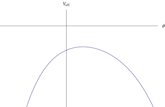
Figure 1: The effective potentials of the dilaton field in the Liouville potential case with (a) $\lambda>0$ and (b) $\lambda<0$.

It should be noted, however, that the “effective potential” is not the ordinary one since it contains metric functions explicitly which depend on $\tilde{r}$. The configuration of the “effective potential” changes depending on $\tilde{r}$, and there is a case where it does not give a right asymptotic behavior, e.g., the dilaton field diverges although the form of the potential is of the type in Fig. 1 (a). Hence we analyse the asymptotic behaviors of the field functions in detail by looking at the asymptotic expansion in the following.

3.3 Asymptotic expansion

Substituting Eqs. (23) into the field equations (9) and (11), one finds the conditions that the leading terms ($\tilde{r}^{2}$ and constant terms in each equation) balance with each other are given by

$$(D)_{3}\gamma\;e^{-\gamma\phi_{0}}\tilde{b}_{2}^{~{}2}+\lambda\tilde{\Lambda}e^{\lambda\phi_{0}}=0\,,$$ (29)

$$(D-1)_{4}\;e^{-\gamma\phi_{0}}\tilde{b}_{2}^{~{}2}-(D-1)_{2}\tilde{b}_{2}-\tilde{\Lambda}e^{\lambda\phi_{0}}=0\,,$$ (30)

which determine $\tilde{b}_{2}$ and $\phi_{0}$, while $\delta_{0}$ can be arbitrary because only its derivative appears in our field equations. Since $\gamma$ is positive and $\tilde{\Lambda}$ is negative, $\lambda$ should be also positive by Eq. (29). This restricts the parameter space to $\lambda>0$. From these equations, we find

$$(D)_{2}\gamma\tilde{b}_{2}+\bigl{[}(D-4)\lambda+D\gamma\bigr{]}\tilde{\Lambda}e^{\lambda\phi_{0}}=0,$$ (31)

$$(D-3)\bigl{[}(D-4)\lambda+D\gamma\bigr{]}\tilde{b}_{2}-\lambda e^{\gamma\phi_{0}}=0.$$ (32)

For $\lambda=\gamma$, the cosmological constant and $\phi_{0}$ are found to be

$$\tilde{\Lambda}=-\frac{(D)_{1}}{4(D-2)_{3}},~{}~{}~{}~{}~{}e^{-\gamma\phi_{0}}\tilde{b}_{2}=\frac{1}{2(D-2)_{3}}.$$ (33)

If we allow the possibility that the dilaton diverges whereas $\tilde{b}_{2}$ becomes infinity, there may be other solutions but the expansion does not give sensible result for such a case. Note that due to the shift symmetry (18), the values of $\phi_{0}$ and $\tilde{b}_{2}$ themselves are not determined individually.

For $\lambda\neq\gamma$, Eqs. (29) and (30) give

$$\tilde{b}_{2}^{~{}2}=\frac{-\lambda\tilde{\Lambda}}{(D)_{3}\gamma}\biggl{[}\frac{D(D-3)}{(D-1)_{2}}(-\tilde{\Lambda})\frac{\gamma}{\lambda}\biggl{(}1+\frac{(D-4)\lambda}{D\gamma}\biggr{)}^{2}\biggr{]}^{\frac{\gamma+\lambda}{\gamma-\lambda}},$$ (34)

$$e^{\phi_{0}}=\biggl{[}\frac{D(D-3)}{(D-1)_{2}}(-\tilde{\Lambda})\frac{\gamma}{\lambda}\biggl{(}1+\frac{(D-4)\lambda}{D\gamma}\biggr{)}^{2}\biggr{]}^{\frac{1}{\gamma-\lambda}}.$$ (35)

The candidates of the next leading terms for Eqs. (9)–(11) are respectively given by

$$2(D-2)\left[\mu-(D-3)\right]\left[1-2(D-3)_{4}\tilde{b}_{2}e^{-\gamma\phi_{0}}\right]\tilde{M}\tilde{r}^{-\mu}$$

$$\hskip 28.45274pt-\Bigl{[}(D-2)_{3}\gamma\tilde{b}_{2}^{2}e^{-\gamma\phi_{0}}\{4\nu^{2}-4(D-2)\nu+(D-1)(D-4)\}+\lambda\tilde{\Lambda}e^{\lambda\phi_{0}}\Bigr{]}\phi_{1}\tilde{r}^{2-\nu}\,,$$ (36)

$$\rule[0.0pt]{0.0pt}{19.91692pt}\Bigl{[}2(D-3)_{4}\tilde{b}_{2}e^{-\gamma\phi_{0}}-1\Bigr{]}\sigma\delta_{1}\tilde{r}^{-\sigma}+2(D-3)\tilde{b}_{2}e^{-\gamma\phi_{0}}\gamma\nu(1+\nu)\phi_{1}\tilde{r}^{-\nu}\,,$$ (37)

$$\rule[0.0pt]{0.0pt}{19.91692pt}4(D-2)_{3}\tilde{b}_{2}^{2}e^{-\gamma\phi_{0}}\gamma\sigma(\sigma-D)\delta_{1}\tilde{r}^{-\sigma}+\Bigl{[}D_{3}\tilde{b}_{2}^{2}e^{-\gamma\phi_{0}}\gamma^{2}-\lambda^{2}\tilde{\Lambda}e^{\lambda\phi_{0}}-\tilde{b}_{2}(D-1)\nu+\tilde{b}_{2}\nu^{2}\Bigr{]}\phi_{1}\tilde{r}^{-\nu}$$

$$\hskip 28.45274pt-4(D-2)_{3}\tilde{b}_{2}e^{-\gamma\phi_{0}}[\mu-(D-2)][\mu-(D-3)]\gamma\tilde{M}\tilde{r}^{-\mu-2}\,,$$ (38)

which should vanish. By use of the leading equations (31) and (32), these equations reduce to

$$\bigl{[}\mu-(D-3)\bigr{]}\bigl{[}(D-4)\lambda-D\gamma\bigr{]}\tilde{M}\tilde{r}^{-\mu}-2\gamma\lambda(\nu+1)\bigl{[}\nu-(D-1)\bigr{]}\tilde{b}_{2}\phi_{1}\tilde{r}^{2-\nu}\,,$$ (39)

$$\rule[0.0pt]{0.0pt}{19.91692pt}\bigl{[}(D-4)\lambda-D\gamma\bigr{]}\sigma\delta_{1}\tilde{r}^{-\sigma}+2\lambda\gamma\nu(\nu+1)\phi_{1}\tilde{r}^{-\nu}\,,$$ (40)

$$\rule[0.0pt]{0.0pt}{19.91692pt}4(D-2)\lambda\gamma\sigma(\sigma-D)\tilde{b}_{2}\delta_{1}\tilde{r}^{-\sigma}$$

$$\hskip 28.45274pt+\Bigl{\{}(D)_{2}\lambda\gamma(\lambda+\gamma)+\bigl{[}(D-4)\lambda+D\gamma\bigr{]}\nu\bigl{[}\nu-(D-1)\bigr{]}\Bigr{\}}\tilde{b}_{2}\phi_{1}\tilde{r}^{-\nu}$$

$$\hskip 28.45274pt+4(D-2)\lambda\gamma\bigl{[}\mu-(D-2)\bigr{]}\bigl{[}\mu-(D-3)\bigr{]}\tilde{M}\tilde{r}^{-\mu-2}\,,$$ (41)

up to overall factors. Now we need to discuss two cases separately.

3.3.1 $(D-4)\lambda-D\gamma\neq 0$ case

Let us first consider the case with $(D-4)\lambda-D\gamma\neq 0$. There are two different classes which give consistent expansions. One is realized when the $\tilde{r}^{-\mu}$ term dominates over other terms. We then find $\mu=D-3$ and $\nu>D-1$ and rename the coefficient $\tilde{M}$ as $\tilde{M}_{0}$.

The other class corresponds to the ordinary modes of the second order differential equation of the dilaton field, where all these terms are of the same order with $\mu=\nu-2=\sigma-2$. From the next leading terms in (39) and (40), we find

$$\bigl{[}(D-4)\lambda-D\gamma\bigr{]}\tilde{M}-2\lambda\gamma(\nu+1)\tilde{b}_{2}\phi_{1}=0\,,$$

$$\rule[0.0pt]{0.0pt}{19.91692pt}\bigl{[}(D-4)\lambda-D\gamma\bigr{]}\delta_{1}+2\lambda\gamma(\nu+1)\phi_{1}=0\,.$$ (42)

Substituting these into the condition obtained from (41)

$$4(D-2)(\nu-D)\lambda\nu\tilde{b}_{2}\delta_{1}+(D)_{2}\lambda\gamma(\lambda+\gamma)\tilde{b}_{2}\phi_{1}$$

$$~{}~{}+\nu(\nu+1-D)\bigl{[}(D-4)\lambda+D\gamma\bigr{]}\tilde{b}_{2}\phi_{1}+4(D-2)(\nu-D)(\nu+1-D)\lambda\gamma\tilde{M}=0,~{}~{}~{}~{}$$ (43)

we find

$$\nu=\nu_{\pm}=\frac{D-1}{2}\left[1\pm\sqrt{1-\frac{4(D)_{2}\lambda\gamma(\lambda-\gamma)\bigl{[}(D-4)\lambda+D\gamma\bigr{]}}{(D-1)^{2}\bigl{[}(D-4)^{2}\lambda^{2}-D^{2}\gamma^{2}-8(D-1)_{2}\lambda^{2}\gamma^{2}\bigr{]}}}\;\right].$$ (44)

The power indices $\nu$, $\mu$ and $\sigma$ do not depend on $\tilde{\Lambda}$. Here we assume

$$(D-4)^{2}\lambda^{2}-D^{2}\gamma^{2}-8(D-1)_{2}\lambda^{2}\gamma^{2}\neq 0,$$ (45)

since otherwise $\nu$ has no solution.

We rewrite the indices $\nu_{\pm}$ as

$$\nu_{\pm}=\frac{D-1}{2}\biggl{[}1\pm\sqrt{1-\frac{{\tilde{m}}^{2}}{{\tilde{m}}_{BF}^{2}}}\biggr{]},$$ (46)

where the mass square of Breitenlohner and Freedman (BF) bound is defined by [21]

$$\tilde{m}_{BF}^{2} =-\frac{(D-1)^{2}}{4\tilde{\ell}_{AdS}^{2}}=-\frac{(D-1)^{2}}{4}\tilde{b}_{2},$$ (47)

and we define the mass square of the dilaton field as

$$\tilde{m}^{2}=-\frac{(D)_{2}\lambda\gamma(\lambda-\gamma)\bigl{[}(D-4)\lambda+D\gamma\bigr{]}}{(D-4)^{2}\lambda^{2}-D^{2}\gamma^{2}-8(D-1)_{2}\lambda^{2}\gamma^{2}}\tilde{b}_{2}.$$ (48)

by the analogy with the discussion in BF bound. This mass is considered to be the second derivative of the potential of the dilaton field where the $\tilde{r}$-dependence of the “effective potential” (25) is taken into account. Not that these equations hold even for the $\gamma=\lambda$ case if the value of the cosmological constant is given by Eq. (33), and $\nu_{\pm}=0,\;D-1$.

Let us now consider the normalizability of the dilaton field. In the ordinary discussion of the BF bound, the normalizable condition [21, 22, 23] is assumed to be $\nu\geq(D-3)/2$. For $\tilde{m}^{2}\geq\tilde{m}_{BF}^{2}+\tilde{\ell}_{AdS}^{-2}$, we find that the $\nu_{-}$ mode is non-normalizable while the $\nu_{+}$ mode is normalizable. Hence the $\nu_{-}$ mode should be tuned to vanish. For $\tilde{m}_{BF}^{2}<\tilde{m}^{2}<\tilde{m}_{BF}^{2}+\tilde{\ell}_{AdS}^{-2}$, both modes are normalizable, and the spacetime has different classes of AdS spacetime asymptotically depending on the ratio of these modes. This normalizability condition does not seem to apply to our case because our dilaton field is not considered to be quantum fluctuations. Nevertheless, we adopt the boundary condition that the $\nu_{-}$ mode vanishes. In the BF bound analysis, it is known that the normalizable modes give finite conserved mass. Although our system is different from such a system due to the GB term and the dilaton coupling, we impose this condition.

We eliminate the $\nu_{-}$ mode by tuning the value of $\phi_{H}$. Hence $\phi_{H}$ is not a free parameter but a kind of shooting parameter and should be chosen suitably for each horizon radius and other theoretical parameters. Also using the symmetry (19), we set $\delta_{0}=0$.

The asymptotic forms of the field functions are then

$$\phi\sim\phi_{0}+\frac{\phi_{+}}{\tilde{r}^{\nu_{+}}}+\cdots\,,$$

$$B\sim\tilde{b}_{2}\tilde{r}^{2}-\frac{2\tilde{M}_{+}}{\tilde{r}^{\nu_{+}-2}}-\frac{2\tilde{M}_{0}}{\tilde{r}^{D-3}}+\cdots\,,$$ (49)

$$\delta\sim\delta_{0}+\frac{\delta_{+}}{\tilde{r}^{\nu_{+}}}+\cdots\,.$$

Note that while $B$ has the term $r^{-\nu_{+}+2}$, the $g_{tt}$ component of the metric behaves as

$$-g_{tt}=Be^{-2\delta}\sim\tilde{b}_{2}\tilde{r}^{2}-\frac{2\tilde{M}_{0}}{\tilde{r}^{D-3}}+\cdots.$$ (50)

(Remember that we have chosen $\delta_{0}=0$.) This value of $\tilde{M}_{0}$ is the gravitational mass of the black holes. Thus it is convenient to define the mass function $\tilde{m}_{g}(\tilde{r})$ by

$$-g_{tt}=\tilde{b}_{2}\tilde{r}^{2}-\frac{2\tilde{m}_{g}(\tilde{r})}{\tilde{r}^{D-3}}.$$ (51)

We will present our results in terms of this function.

3.3.2 $(D-4)\lambda-D\gamma=0$ case

In this case, from Eqs. (42), we find $\nu=-1$. This is a growing mode which means that the expansion is not valid. We have then examined next order equations, but did not obtain any other non-growing modes. Thus this case does not seem to give sensible solutions. Hence we do not consider this case.

3.4 Allowed parameter regions

In this subsection, using the above results, we discuss the parameter regions which give desirable black hole solutions.

The mass of the dilaton field $\tilde{m}$ should satisfy the conditions

$$\tilde{m}_{BF}^{2}\leq\tilde{m}^{2},$$ (52)

which comes from that the stability of the asymptotic structure of the solution against time-dependent perturbations. This implies that the parameters $\gamma$ and $\lambda$ should satisfy

$$\frac{4(D)_{2}\lambda\gamma(\lambda-\gamma)\bigl{[}(D-4)\lambda+D\gamma\bigr{]}}{(D-1)^{2}\bigl{[}(D-4)^{2}\lambda^{2}-D^{2}\gamma^{2}-8(D-1)_{2}\lambda^{2}\gamma^{2}\bigr{]}}\leq 1.$$ (53)

The regions in which these conditions (53) are satisfied is depicted in Fig. 2. Remember that we are considering only the region $\gamma>0$, $\lambda>0$.

We also impose another condition

$$\tilde{m}^{2}<0.$$ (54)

When $\tilde{m}^{2}>0$, the potential of the dilaton field is an ordinary (non-tachyonic) convex potential, and there is a growing mode according to Eq. (46). Such a mode should be eliminated by tuning $\phi_{H}$ at the horizon for the finiteness of the dilaton field. The solution must be stable against time-dependent perturbations since the condition of BF bound (52) is satisfied. By the numerical analysis, however, we find that the growing mode cannot be eliminated just by tuning $\phi_{H}$, and the dilaton field diverges. Although this fact does not mean that there cannot be a solution with $\tilde{m}^{2}<0$ for any parameters $\gamma$ and $\lambda$, we impose the condition (54) in this paper. Then the potential of the dilaton field is tachyonic, and the dilaton field climbs up the potential slope asymptotically. The condition (54) is rewritten as

$$\lambda<\gamma,$$ (55)

or

$$\lambda>\frac{D\gamma}{\sqrt{(D-4)^{2}-8(D-1)_{2}\gamma^{2}}}~{}~{}~{}\mbox{and}~{}~{}~{}0<\gamma<\frac{D-4}{\sqrt{8(D-1)_{2}}}\;.$$ (56)

These regions are depicted in Fig. 3.

By superposing Figs. 2 and 3, we find that there are two separate allowed regions in the parameter space $(\lambda,\gamma)$. This is shown in Fig. 4. There is a narrow region near $\gamma=0$ axis, but we did not find any relevant solutions with parameters in this region when we integrate the basic equations outwards from the event horizon numerically. Since these conditions are obtained by the asymptotic behaviors of the field functions, it is expected that they do not extend there because the spacetime hits singularity before reaching the asymptotic region.

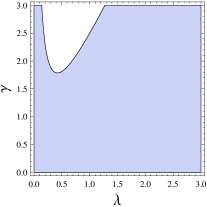
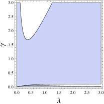
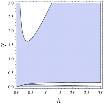
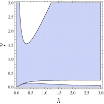
Figure 2: The allowed regions for the parameters $\gamma$ and $\lambda$ from the condition (53) for (a) $D=4$, (b) $D=5$, (c) $D=6$, and (d) $D=10$.

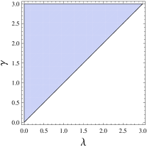
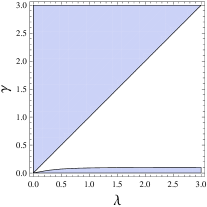
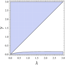
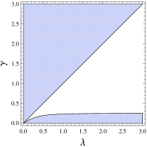
Figure 3: The allowed regions for the parameters $\gamma$ and $\lambda$ from the condition (54) for (a) $D=4$, (b) $D=5$, (c) $D=6$, and (d) $D=10$.

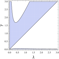
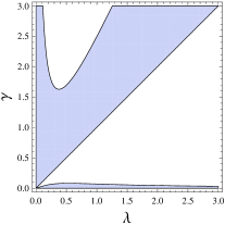
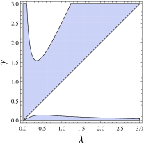
Figure 4: The allowed regions from the conditions (53) and (54) for (a) $D=4$, (b) $D=5$, (c) $D=6$, and (d) $D=10$.

4 Black hole solutions

The basic equations (9)–(11) do not have analytical solutions, so we have to resort to the numerical method. In the numerical analysis, we have to first choose the parameters for our black hole solutions from the allowed regions of $\gamma$ and $\lambda$, and other parameters. Considering the results in the previous section, we choose the following parameters and conditions as a typical example in various dimensions:

$$\gamma=\frac{1}{2},~{}~{}\lambda=\frac{1}{3},~{}~{}\tilde{\Lambda}<0,~{}~{}\phi_{-}=0,~{}~{}\delta_{0}=0,$$ (57)

and expect that this choice gives the typical solutions. In fact, it should not be difficult to get solutions for other choice if it is in the allowed region.

We next fix the radius of the event horizon $\tilde{r}_{H}$ and the cosmological constant $\tilde{\Lambda}$. We then choose the value of the dilaton field $\phi_{H}$ at the horizon, and determine the values of other fields by (22). Among these, $\phi_{H}$ should be tuned such that $\phi_{-}=0$ in the asymptotic behavior (49). Hence there is only one freedom of choosing $\tilde{r}_{H}$, given a cosmological constant.

Once a solution for one $\tilde{r}_{H}$ and a fixed cosmological term is obtained, we can get solutions for different $\tilde{r}_{H}$ but with the same $\tilde{\Lambda}$ by using the transformation (17). Under this transformation, we have

$$\tilde{r} \to \hat{r}\equiv a\tilde{r},$$

$$B(\tilde{r}) \to \hat{B}(\hat{r})\equiv a^{2}B(\tilde{r}),$$ (58)

$$~{}~{}~{}~{}~{}~{}=a^{2}\Bigg{[}\tilde{b}_{2}(\hat{r}/a)^{2}-\frac{2\tilde{M_{+}}}{(\hat{r}/a)^{\nu_{+}-2}}-\frac{2\tilde{M}_{0}}{(\hat{r}/a)^{D-3}}\Bigg{]}$$

$$~{}~{}~{}~{}~{}~{}=\tilde{b}_{2}\hat{r}^{2}-\frac{2a^{\nu_{+}}\tilde{M}_{+}}{\hat{r}^{\nu_{+}-2}}-\frac{2a^{D-1}\tilde{M}_{0}}{\hat{r}^{D-3}}.$$

Thus the gravitational mass scales like $a^{D-1}\tilde{M}_{0}$. This means that the mass $\tilde{M}_{0}$ depends on the horizon radius as

$$\tilde{M}_{0}\propto\tilde{r}_{H}^{\;D-1},$$ (59)

for a fixed cosmological constant.

Given a solution for a cosmological constant, we can generate solutions for different cosmological constants but the same $\tilde{r}_{H}$ by using transformation (18). Suppose that we get a solution for a certain $\tilde{\Lambda}$ and a fixed $\tilde{r}_{H}$. Using Eq. (18), we get a new solution by

$$B\to a^{2\gamma/(\gamma-\lambda)}B,~{}~{}\phi\to\phi+\frac{2}{\gamma-\lambda}\ln a,~{}~{}\tilde{\Lambda}\to a^{2}\tilde{\Lambda}.$$ (60)

Note that this does not shift $\phi_{-}$ in the asymptotic expansion (49), so the condition $\phi_{-}=0$ is not spoiled. Under this transformation, the mass changes as

$$\tilde{M}_{0}\to a^{2\gamma/(\gamma-\lambda)}\tilde{M}_{0}.$$ (61)

This means that when the cosmological constant is changed, the mass scales like

$$\tilde{M}_{0}\propto|\tilde{\Lambda}|^{\gamma/(\gamma-\lambda)},$$ (62)

independently of our spacetime dimension. When the condition (55) is satisfied, the power of $\tilde{\Lambda}$ is positive. Thus the mass becomes larger as the magnitude of the cosmological constant becomes larger. For our choice $\gamma=1/2$ and $\lambda=1/3$, this gives $\tilde{M}_{0}\sim|\tilde{\Lambda}|^{3}$.

As in our previous paper, [1] we present our solutions for $D=4,5,6$ and 10 because those in $D=7,8,9$ are similar to the solution in $D=10$.

4.1 Non-dilatonic case

It will be instructive to compare our results with the non-dilatonic case. So let us derive some physical quantities for this case here. When the dilaton field is absent (i.e., Einstein-Gauss-Bonnet system with cosmological constant), we substitute $\phi\equiv 0$ and $\gamma=0$ into Eqs. (9) and (10), which can then be integrated to yield

$$B(\tilde{r})=\frac{1}{2(D-3)_{4}}\left(1\mp\sqrt{1-\frac{4(D-3)_{4}}{\tilde{\ell}^{2}}+\frac{8(D-3)_{4}\bar{M}}{\tilde{r}^{D-1}}}\,\right)\tilde{r}^{2},$$ (63)

$$\delta({\tilde{r}})\equiv 0$$ (64)

where $\bar{M}$ is an integration constant related to the conserved mass of the black hole. [24] The solutions in minus branch have black hole horizon and approaches the solutions in general relativity in the $\alpha_{2}\to 0$ limit. Hence this is the general relativity (GR) branch. The solutions in the plus branch do not have a event horizon and the spacetime is naked singular. This is called the GB branch. The condition $B(\tilde{r}_{H})=0$ gives the relation between $\tilde{M}$ and $\tilde{r}_{H}$ as

$$\bar{M}=\frac{1}{2\tilde{\ell}^{2}}\tilde{r}_{H}^{\;D-1}.$$ (65)

This dependence is the same as Eq. (59). In the pure vacuum (source-less) spacetime $\bar{M}=0$, we have

$$B(\tilde{r})=\frac{1}{2(D-3)_{4}}\left(1\mp\sqrt{1-\frac{4(D-3)_{4}}{\tilde{\ell}^{2}}}\,\right)\tilde{r}^{2}\equiv\frac{\tilde{r}^{2}}{\bar{\ell}_{\rm AdS}^{2}},$$ (66)

where $\bar{\ell}_{\rm AdS}^{2}$ is square of the AdS curvature radius in the non-dilatonic case given as

$$\bar{\ell}_{\rm AdS}^{2}=\frac{\bar{\ell}^{2}}{2}\left(1\pm\sqrt{1-\frac{4(D-3)_{4}}{\bar{\ell}^{2}}}\>\right).$$ (67)

It is then natural to define the new mass function $\tilde{\mu}$ (gravitational mass) by

$$B(\tilde{r})=\frac{\tilde{r}^{2}}{\bar{\ell}_{\rm AdS}^{2}}-\frac{2\tilde{\mu}(\tilde{r})}{\tilde{r}^{D-3}}\,,$$ (68)

By Eq. (63),

$$\tilde{\mu}(\tilde{r})=\pm\frac{1}{4(D-3)_{4}}\Biggl{[}\sqrt{1-\frac{4(D-3)_{4}}{\tilde{\ell}^{2}}+\frac{8(D-3)_{4}\bar{M}}{\tilde{r}^{D-1}}}-\sqrt{1-\frac{4(D-3)_{4}}{\tilde{\ell}^{2}}}\Biggr{]}\tilde{r}^{D-1},$$ (69)

where the plus and minus signs are for the GR and the GB branches respectively. The asymptotic value $\tilde{\mu}(\infty)$, which corresponds to the gravitational mass, is related to $\bar{M}$ by $\bar{M}=\pm\tilde{\mu}(\infty)\sqrt{1-{4(D-3)_{4}}/{\tilde{\ell}^{2}}}$.

4.2 $D=4$ solution

We first present the black hole solutions for $D=4$. For the horizon radius $\tilde{r}_{H}=1$ and $\tilde{\Lambda}=-3/2$ $(\tilde{\ell}=2)$ with the additional boundary conditions (22) at the horizon, we integrate the field equations from the event horizon to infinity. Then we find $\phi_{H}=2.33422$ in order to obtain $\phi_{-}=0$ as given in Eq. (57), and $\delta_{H}=-0.02893$, $\phi_{0}=2.43279$ and $\tilde{M}_{0}=0.28014$. The behaviors of $\tilde{m}_{g}$ (defined in Eq. (51)), $\delta$ and $\phi$ as functions of $\tilde{r}$ are depicted in Fig. 5. This solution corresponds to the dilatonic version of the minus branch solution in the non-dilatonic case. We cannot find the counterpart of the plus branch in non-dilatonic solution. Solutions for other $\tilde{r}_{H}$ and cosmological constants is obtained from this solution by the transformations (58) and (60), respectively. It follows from Eqs. (59) and (62) that the gravitational mass $\tilde{M}_{0}$ is given by

$$\tilde{M}_{0}=0.28014\biggl{(}\frac{2|\tilde{\Lambda}|}{3}\biggr{)}^{\!3}\tilde{r}_{H}^{\;3}\,.$$ (70)

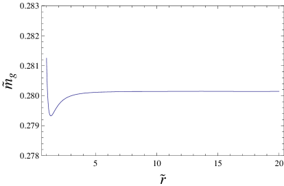
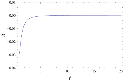
Figure 5: The configurations of the field functions (a) $\tilde{m}_{g}$, (b) $\delta$ and (c) $\phi$ in four dimensions for $\tilde{r}_{H}=1$ and $\tilde{\Lambda}=-3/2$.

4.3 $D=5$ solution

For the horizon radius $\tilde{r}_{H}=1$ and $\tilde{\Lambda}=-3$ $(\tilde{\ell}=2)$ with the additional boundary conditions (22) at the horizon, we find $\phi_{H}=9.35869$ in order to obtain $\phi_{-}=0$. Then we find $\delta_{H}=-0.02188,\phi_{0}=9.43249$ and $\tilde{M}_{0}=3.78189$. The behaviors of $\tilde{m},\delta$ and $\phi$ as functions of $\tilde{r}$ are depicted in Fig. 6. Solutions for other $\tilde{r}_{H}$ and cosmological constants may be obtained from this solution by the transformations (58) and (60), respectively. The gravitational mass $\tilde{M}_{0}$ is given by the rules (59) and (62) as a function of the cosmological constant $\tilde{\Lambda}$ and the horizon radius $\tilde{r}_{H}$:

$$\tilde{M}_{0}=3.7819\biggl{(}\frac{|\tilde{\Lambda}|}{3}\biggr{)}^{\!3}\tilde{r}_{H}^{\;4}\,.$$ (71)

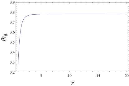
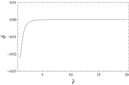
Figure 6: The configurations of the field functions (a) $\tilde{m}_{g}$, (b) $\delta$ and (c) $\phi$ in five dimensions for $\tilde{r}_{H}=1$ and $\tilde{\Lambda}=-3$.

4.4 $D=6$ solution

For the horizon radius $\tilde{r}_{H}=1$ and $\tilde{\Lambda}=-5$ $(\tilde{\ell}=2)$ with the additional boundary conditions (22) at the horizon, we find $\phi_{H}=13.8108$ in order to obtain $\phi_{-}=0$. Then we find $\delta_{H}=-0.01621,\phi_{0}=13.86530$ and $\tilde{M}_{0}=19.93321$. The behaviors of $\tilde{m},\delta$ and $\phi$ as functions of $\tilde{r}$, which are depicted in Fig. 7. Solutions for other $\tilde{r}_{H}$ and cosmological constants may be obtained from this solution by the transformations (58) and (60), respectively. The gravitational mass $\tilde{M}_{0}$ is given by the rules (59) and (62) as a function of the cosmological constant $\tilde{\Lambda}$ and the horizon radius $\tilde{r}_{H}$:

$$\tilde{M}_{0}=19.933\biggl{(}\frac{|\tilde{\Lambda}|}{5}\biggr{)}^{\!3}\tilde{r}_{H}^{\;5}\,.$$ (72)

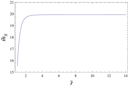
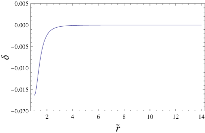
Figure 7: The configurations of the field functions (a) $\tilde{m}$, (b) $\delta$ and (c) $\phi$ in six dimensions for $\tilde{r}_{H}=1$ and $\tilde{\Lambda}=-5$.

4.5 $D=10$ solution

For the horizon radius $\tilde{r}_{H}=1$ and $\tilde{\Lambda}=-18$ $(\tilde{\ell}=2)$ with the additional boundary conditions (22) at the horizon, we find $\phi_{H}=23.6338$ in order to obtain $\phi_{-}=0$ as given in Eq. (57). Then we find $\delta_{H}=-0.0024575,\phi_{0}=23.64366$ and $\tilde{M}_{0}=771.67622$. The behaviors of $\tilde{m},\delta$ and $\phi$ as functions of $\tilde{r}$, are depicted in Fig. 8. Solutions for other $\tilde{r}_{H}$ and cosmological constants may be obtained from this solution by the transformations (58) and (60), respectively. The gravitational mass $\tilde{M}_{0}$ is given by the rules (59) and (62) as a function of the cosmological constant $\tilde{\Lambda}$ and the horizon radius $\tilde{r}_{H}$:

$$\tilde{M}_{0}=771.68\biggl{(}\frac{|\tilde{\Lambda}|}{18}\biggr{)}^{\!3}\tilde{r}_{H}^{\;9}\,.$$ (73)

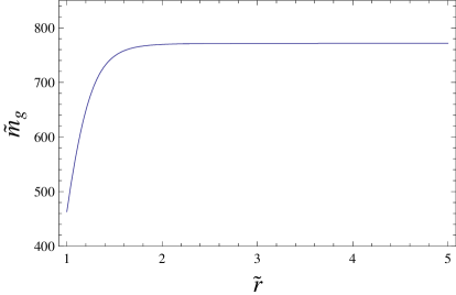
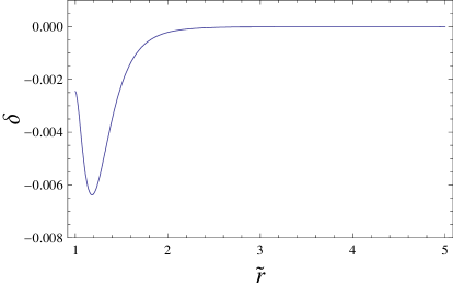
Figure 8: The configurations of the field functions (a) $\tilde{m}$, (b) $\delta$ and (c) $\phi$ in ten dimensions for $\tilde{r}_{H}=1$ and $\tilde{\Lambda}=-18$.

5 Conclusions and Discussions

We have studied the black hole solutions in dilatonic Einstein-GB theory with the negative cosmological constant. The cosmological constant introduces the Liouville type of potential for the dilaton field. We have taken the plane symmetric spacetime, i.e., the $(D-2)$-dimensional hypersurface spanned by the angular coordinates with vanishing constant curvature ($k=0$). The basic equations have some symmetries which are used to generate the black hole solutions with different horizon radius and the cosmological constant.

We have also examined the boundary conditions at the horizon and found that there is no asymptotically AdS solution unless we introduce the cosmological constant. By the asymptotic expansion at infinity, the power decaying rate of the field variables are estimated. We have imposed the condition that the “mass” of the dilaton field satisfies the BF bound, which guarantees the stability of the vacuum solution. By this condition, the values of the dilaton coupling constant and the parameter of the Liouville potential are constrained. For a typical choice of the parameters and boundary conditions, we were able to construct AdS black hole solutions in various dimensions.

In the non-dilatonic case, there are two analytical solutions, one of which is the black hole solutions (GR branch) and the other is the solution with the naked singularity (GB branch). In the dilatonic case, we have chosen $\gamma=1/2$ and $\lambda=1/3$ for the actual numerical analysis. The black hole solutions are constructed in $D=4,5,6$ and $10$. We have checked that the dilaton field climbs up its potential slope and takes constant values at infinity. We have found that the relation of the gravitational mass and the horizon radius of the black hole is

$$\tilde{M}_{0}\propto|\tilde{\Lambda}|^{\gamma/(\gamma-\lambda)}\tilde{r}_{H}^{\;D-1}\,.$$ (74)

There are some remaining issues left for future works. One of them is the thermodynamics of our black holes. The Hawking temperature is given by the periodicity of the Euclidean time on the horizon as

$$\tilde{T}_{H}~{} =\frac{e^{-\delta_{H}}}{4\pi}B_{H}^{\prime}$$ (75)

$$=-\frac{e^{-\delta_{H}}}{4(D-2)\pi}\tilde{\Lambda}\tilde{r}_{H}e^{\lambda\phi_{H}},$$

where the first equality holds for any $k$ but we set $k=0$ in obtaining the second line. It follows from the scaling symmetry (17) that the temperature is proportional to the horizon radius. In the case of GB gravity, the entropy is not obtained by a quarter of the area of the event horizon. Along the definition of entropy in Ref. Wald, which originates from the Noether charge associated with the diffeomorphism invariance of the system, we obtain

$$\tilde{S}=\frac{\tilde{r}_{H}^{D-2}\Sigma_{k}}{4}\left[1+2(D-2)_{3}\frac{ke^{-\gamma\phi_{H}}}{\tilde{r}_{H}^{2}}\right]-\tilde{S}_{min},$$ (76)

where $S_{min}$ is added to make the entropy non-negative[26]. (See also Ref. CNO.) For the plane symmetric case $k=0$, we can set $S_{min}=0$, and the entropy is proportional to $\tilde{r}_{H}^{\>D-2}$. The $\tilde{r}_{H}$ dependence of the temperature and entropy shows that the thermodynamical mass is estimated as $\tilde{M}_{thermo}\propto\tilde{r}_{H}^{\;D-1}$ by the first law of black hole thermodynamics if we assume that the zero size black hole has zero mass. This is same as that of the gravitational mass.

In this paper, we have assumed that $\tilde{m}^{2}<0$, which means that there is no growing mode of the dilaton field asymptotically. However, even for the case with $\tilde{m}^{2}>0$, the growing mode may be turned off by tuning the boundary value $\phi_{H}$. The dilaton field of such solution is normalizable and decays faster than that of the solutions presented in this paper. Furthermore, the solution must be stable by the form of the non-tachyonic potential. Hence it will be physically relevant. The search for this solutions is left for future work. On the other hand, even if the solution has a growing mode, when the dilaton field diverges minus infinity and $\tilde{b}_{2}=0$, the system reduces to GR. This situation is similar to Ref. cai. The relevance of such solution should be investigated further.

It would be also interesting to extend our work to other spacetimes, including $k=1$ and other topological black holes with the cosmological constant. We plan to report our results on these cases in the future publication.

Finally we hope that our asymptotically AdS black hole solutions are useful for examining properties of field theories via AdS/CFT correspondence.

References

- [1] Z. K. Guo, N. Ohta and T. Torii, Prog. Theor. Phys. 120 (2008) 581 [arXiv:0806.2481 [gr-qc]].
- [2] G. W. Gibbons and K. Maeda, Nucl. Phys. B298 (1988) 741.
- [3] D. Garfinkle, G. T. Horowitz, and A. Strominger, Phys. Rev. D 43 (1991) 3140.
-
[4]
D. J. Gross and J. H. Sloan,
Nucl. Phys. B 291 (1987) 41;
M. C. Bento and O. Bertolami, Phys. Lett. B 368 (1996) 198. - [5] P. Kanti, N. E. Mavromatos, J. Rizos, K. Tamvakis and E. Winstanley, Phys. Rev. D 54 (1996) 5049 [arXiv:hep-th/9511071].
- [6] S. O. Alexeev and M. V. Pomazanov, Phys. Rev. D 55 (1997) 2110 [arXiv:hep-th/9605106].
- [7] T. Torii, H. Yajima and K. Maeda, Phys. Rev. D 55 (1997) 739 [arXiv:gr-qc/9606034].
- [8] C. M. Chen, D. V. Gal’tsov and D. G. Orlov, Phys. Rev. D 75 (2007) 084030 [arXiv:hep-th/0701004].
- [9] C. M. Chen, D. V. Gal’tsov and D. G. Orlov, arXiv:0809.1720 [hep-th].
- [10] D. G. Boulware and S. Deser, Phys. Rev. Lett. 55 (1985) 2656.
-
[11]
J. T. Wheeler,
Nucl. Phys. B 268 (1986) 737;
D. L. Wiltshire, Phys. Lett. B 169 (1986) 36;
R. C. Myers and J. Z. Simon, Phys. Rev. D 38 (1988) 2434;
G. Giribet, J. Oliva and R. Troncoso, JHEP 0605 (2006) 007 [arXiv:hep-th/0603177];
R. G. Cai and N. Ohta, Phys. Rev. D 74 (2006) 064001 [arXiv:hep-th/0604088].
For reviews and references, see C. Garraffo and G. Giribet, arXiv:0805.3575 [gr-qc] and C. Charmousis, arXiv:0805.0568 [gr-qc]. - [12] R. G. Cai, Phys. Rev. D 65 (2002) 084014 [arXiv:hep-th/0109133].
- [13] J. Polchinski, “String theory,” Cambridge Univ. Pr. (1998).
-
[14]
S. J. Poletti and D. L. Wiltshire,
Phys. Rev. D 50 (1994) 7260
[Erratum-ibid. D 52 (1995) 3753]
[arXiv:gr-qc/9407021];
S. J. Poletti, J. Twamley and D. L. Wiltshire, Phys. Rev. D 51 (1995) 5720 [arXiv:hep-th/9412076]. - [15] K. C. K. Chan, J. H. Horne and R. B. Mann, Nucl. Phys. B 447 (1995) 441 [arXiv:gr-qc/9502042].
- [16] C. Charmousis, Class. Quant. Grav. 19 (2002) 83 [arXiv:hep-th/0107126].
- [17] L. Alvarez-Gaume, P. H. Ginsparg, G. W. Moore and C. Vafa, Phys. Lett. B 171 (1986) 155.
- [18] K. Bamba, Z. K. Guo and N. Ohta, Prog. Theor. Phys. 118 (2007) 879 [arXiv:0707.4334 [hep-th]].
- [19] M. Henneaux and C. Teitelboim, Comm. Math. Phys. 98 (1985) 391.
- [20] T. Torii, K. Maeda and M. Narita, Phys. Rev. D 64 (2001) 044007.
- [21] P. Breitenlohner and D. Z. Freedman, Annals Phys. 144 (1982) 249.
- [22] T. Hertog and K. Maeda, JHEP 0407 (2004) 051 [arXiv:hep-th/0404261].
- [23] V. Balasubramanian, P. Kraus, and A. Lawrence Phys. Rev. D 59 (1999) 046003 [arXiv:hep-th/9805171].
- [24] S. Deser and B. Tekin, Phys. Rev. D 67 (2003) 084009 [arXiv:hep-th/0212292].
-
[25]
R. M. Wald,
Phys. Rev. D 48 (1993) 3427
[arXiv:gr-qc/9307038];
V. Iyer and R. M. Wald, Phys. Rev. D 50 (1994) 846 [arXiv:gr-qc/9403028]. - [26] T. Clunan, S. F. Ross and D. J. Smith, Class. Quant. Grav. 21 (2004) 3447 [arXiv:gr-qc/0402044].
- [27] M. Cvetic, S. Nojiri and S. D. Odintsov, Nucl. Phys. B 628 (2002) 295 [arXiv:hep-th/0112045].
- [28] R. G. Cai and A. Wang, Phys. Rev. D 70 (2004) 084042 [arXiv:hep-th/0406040].