Also at ]Physics Department, Grupo de Simulacion de Sistemas Fisicos. Universidad Nacional de Colombia.

3D Molecular dynamics simulations using spheropolytopes

Abstract

We present a simple and efficient method to simulate three-dimensional, complex-shaped, interacting bodies. The particle shape is represented by Minkowski operators. A time-continuous interaction between these bodies is derived using simple concepts of computational geometry. The model (particles + interactions) is efficient, accurate and easy to implement, and it complies with the conservation laws of physics. 3D simulations of hopper flow shows that the non-convexity of the particles strongly effects the jamming on granular flow.

Molecular Dynamics, MD is the art of modeling complex systems as a collection of particles interacting each other. MD in three-dimensions using arbitrary particle shape is a fundamental problem in several disciplines: Drug molecules often act as a key in a lock formed by a protein cavity, so that they can be designed using MD simulations Carlson and Mccammon (2000); Liquid crystals consisting of complex-shaped molecules exhibit transition to a nematic phase, which can be investigated from particle-based simulations of complex shaped objectsPelzl et al. (1999); The large scale modeling of geological materials in foundations, landslides and fault zones requires a constitutive equation which can be constructed using MD-like models  Alonso-Marroquin et al. (2005); Computing the motion of rigid and articulated bodies can lead to new advances in robotics, automation Mirtich (1998) and virtual reality applications Ruspini and Khatib (2001).

The most typical approach for these applications is to solve the dynamics of interacting rigid bodies, where their real shapes are approximated by polyhedra Mirtich (1998); Baraff (1993); Hasegawa and Sato (2004). The most difficult aspect for the simulations is to model contact interactions. Contact force methods have been proposed for two-dimensional (2D) models using polygonsAlonso-Marroquin et al. (2005); Poeschel and Schwager (2004). However, the extension of this method to three-dimensional (3D) simulations has proven to be extremely difficult. In the simple case of convex polygons, the force is calculated as a function of their overlap area Alonso-Marroquin et al. (2005). However, the assumption that elastic force is a function of their overlap leads to a non-conservative elastic interaction Poeschel and Schwager (2004). An alternative approach is to assume that the potential elastic energy is a function of the overlap. Then forces and torques are derived from this potential Poeschel and Schwager (2004). Both approaches have still not been extended to 3D, because the calculation of the overlap between two polyhedra is computationally very expensive. This is the main reason why most of the commercial codes for particulate systems are still based on simulations with spheres, or clumps of spheres representing complex shaped objects Lu and McDowell (2007).

An alternative solution for the 2D simulations of complex shaped particles has been proposed recently Alonso-Marroquin (2008). The method introduces the concept of spheropolygons, which is the object resulting from dilating a polygon by an sphere. The method not only guarantees energy balance but also proves to be much more efficient that previous models to represent complex particle shape Alonso-Marroquin and Wang (2008); Galindo-Torres and Alonso-Marroquin (2008). In 3D models, the dilation of a polyhedra by a sphere has a precise mathematical meaning using the Minkowski operator. In our knowledge, Liebling and Pournin were the first to introduce the Minkowski operators in particle-based simulations Pournin et al. (2005); Pournin and Liebling (2005). In order to calculate the interactions, they assumed a single contact point between the particles Pournin et al. (2005). These approach, however, leads to forces discontinuous in time and numerical artifacts such as abrupt creation of mechanical energy. An alternative approach is proposed by Pournin by calculating the overlap area between the particles Pournin (2005). This approach in practice is not feasible due to the high complexity of the boundary of the spheropolyhedra.

Figure 1: The spherotetrahedron (right) is obtained by sweeping an sphere into a tetrahedron (left).

In this Letter we present a solution to this problem by using the concept of spheropolytopes. They are generated from the Minkowski addition of a polytope by an sphere, which is nothing more than the object resulting from sweeping a sphere around a polytope. A polytope is a generic mathematical concepts that can refer to polygons, polyhedra or polygonal curves in 3D. The polytope is regarded as a collection of features in the three-dimensional Euclidian space: vertices, edges and faces. The interaction between two spheropolytopes is calculated as a function of the distance between their features. The molecular dynamics is implemented in a simple, efficient and elegant algorithm, which complies with conservation laws of physics. We believe that this model will lead to a wide range of applications of molecular dynamics, as complex particle shape and realistic interactions can be captured in a unified framework using well established concepts of molecular dynamics and computational geometry.

For the representation of arbitrary shaped particles we introduce the mathematical concept of Minkowski sum. Given two sets of points P and Q in an Euclidean space, their Minkowski sum is given by $P\oplus Q=\{\vec{x}+\vec{y}~{}|~{}\vec{x}\in P,~{}\vec{y}\in Q\}$. This operation is geometrically equivalent to the sweeping of one set around the profile of the other without changing the relative orientation (Fig 1). Examples of Minkowski sums are the spheropolygons (sphere $\oplus$ polygons) Alonso-Marroquin (2008), spherocyllinder (sphere $\oplus$ line segment) Pournin et al. (2005), the spherosimplex (sphere $\oplus$ simplex) Pournin and Liebling (2005) and the spheropolyhedron (sphere $\oplus$ polyhedron) Pournin (2005), All these objects can be enclosed in the generic shape of spheropolytopes, which consists of a set of vertices ${V_{i}}$, edges ${E_{i}}$, polygonal faces ${F_{i}}$ and the radius $r$ of the sweeping sphere wich will be called sphero-radius. The three examples of spheropolytopes we will consider in this letter is the rice, the tetra and the yermis in the Fig. 2.

Figure 2: Spheropolytopes generated as sphere $\oplus$ line segment (rice), sphere $\oplus$ tetrahedron ( tetra) and sphere $\oplus$ polyline (yermis).

For the calculation of the contact force between spheropolytopes, we require expressions for the distance between their features. Given two features $G_{i}$ and $G_{j}$ of the spheropolytopes $i$ and $j$, their distance is defined as $d(G_{i},G_{j})=||\vec{X}_{i}-\vec{X}_{j}||$, where $\vec{X}_{i}$ and $\vec{X}_{j}$ is the closest points belonging to either feature. We start with the formula of the distance between a vertex $V_{i}$ and an edge $E_{j}$. Let’s consider the line $\ell_{i}$ containing the edge. First we calculate the closest point of this line to the vertex. if the point lies on the edge this is the closest point of the edge to the vertex. Otherwise we take the minimal of the distance from the vertex to both endings of the edge.

Next we consider the distance between two edges $E_{i}$ and $E_{j}$. Let’s the lines $\ell_{i}$ and $\ell_{j}$ containing the edges, we find the two points on these lines whose distance is minimal. If both points belong to the edges, they define the minimal distance between the edges. Otherwise the distance between the two edges is calculated as the minimal of the distance between each vertex of one edge and the other edge.

For the calculation of the distance between a vertex $V_{i}$ and and face $F_{j}$ we consider the plane $\Pi_{j}$ containing the face. First we project the point on the plane. If the projection of the point in the plane lies inside the polygon face then the distance is calculated between these two points. If the projection lies outside the polygon then the distance is calculated to the closest point in the polygon boundary.

These formulas of distance are used to calculate the force between two spheropolytopes. the force $\vec{F}_{ij}$ on the i-spheropolytope by the j-spheropolytope is taken as a superposition of the interaction between each pair of edges $\vec{F}(E_{i},E_{j})$ and each pair of vertex-face $\vec{F}(V_{i},F_{j})$ for the spheropolytope pair,

$$\vec{F}_{ij}=\sum_{E_{i},E_{j}}\vec{F}(E_{i},E_{j})+\sum_{V_{i},F_{j}}\vec{F}(V_{i},F_{j})+\sum_{V_{j},F_{i}}\vec{F}(V_{j},F_{i}).$$ (1)

The force $F(G_{i},G_{j})$ associated to the two features (edge-edge or vertex-face) is assumed to depend on the overlapping length $\delta$ between them

$$\delta(G_{i},G_{j})=R_{i}+R_{j}-d(G_{i},G_{j}),$$ (2)

with $d(G_{i},G_{j})$ the distance between the features of the spheropolytopes $R_{i}$ the spheroradius of the i-th spheropolytope. The point of contact between the two features is calculated by taken the spheres of radius $R_{i}$ and $R_{j}$ centered in the closest points $\vec{X}_{i}$ and $\vec{X}_{j}$, and finding the intersection between the line connecting these two points and the line connecting the two intersection points of the spheres. This contact point results as

$$\vec{R}(G_{i},G_{j})=\vec{X}_{i}+\frac{R_{i}^{2}-R_{j}^{2}+d^{2}(G_{i},G_{j})}{2d(G_{i},G_{j})}\vec{n},$$ (3)

where $\vec{n}=\frac{\vec{X}_{j}-\vec{X}_{i}}{||\vec{X}_{j}-\vec{X}_{i}||}$. From the point of application of the contact forces we get the torque on the i-spheropolytope by the j-spheropolytope:

$$\vec{\tau}_{ij}=\sum_{E_{i},E_{j}}\vec{\tau}(E_{i},E_{j})+\sum_{V_{i},F_{j}}\vec{\tau}(V_{i},F_{j})+\sum_{V_{j},F_{i}}\vec{\tau}(V_{j},F_{i}).$$ (4)

where

$$\vec{\tau_{i}}(G_{i},G_{j})=(\vec{R}(G_{i},G_{j})-\vec{r}_{i})\times\vec{F}(G_{i},G_{j})$$ (5)

with $\vec{r}_{i}$ the center of mass of the i-spheropolyhedron.

Since the formulas of distance are continuous functions on the degrees of freedom of the spheropolytopes, the total force is continuous too. This avoids the problems of discontinuity in time of the forces in previous models Mirtich (1998). Different forces can be included in this model: for example, a force derived from a potential function of the distance leads to a conservative systems; forces depending on the relative velocities at the contact points leads to dissipative granular materials; Forces depending on the history of relative velocity at the contacts represent frictional granular systems; more sophisticated forces can be used to simulate biomolecules. The electrostatic interaction between the molecules can be modeled by allowing the force depend on the closest points between the features.

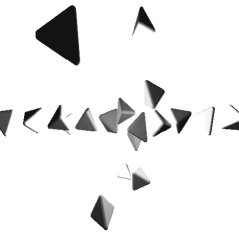
Figure 3: Spherotetrahedra collider for checking the conservation laws.

The first numerical experiment presented in this paper is the spheropolytopes collider (SPC). The simulation consists of colliding opposing beams of spheropolytopes. We consider the three shapes shown in Fig. 2 . The SPC is build with the intention to produce enough collisions to test the basic conservative laws of physics: the conservation of energy, linear and angular momentum. The experimental setup is showed in Fig. 3, two rows of spherotetrahedra are set in a collision course with random orientation and angular velocity. The contact force between features is calculated as

$$\vec{F}(G_{i},G_{j})=-k_{n}\delta(G_{i},G_{j})\vec{n},$$ (6)

where $k_{n}$ is the elastic constant. Once all the forces are calculated we integrate Newton’s second law using the Verlet algorithm for the translation coordinates. The Euler equations form angular momentum is integrated using and the Fincham Leap Frog algorithm, based on the quaternion formalism, for the orientation coordinates Wang et al. (2006). The Table 1 shows the percentage error of the three conservation laws (energy, linear and angular momentum) for two different time steps. The consistency of our numerical method is verify as the error decreases as the time step is smaller. The discretization error is larger in the yermis-particles, because they produce much more collisions than the other particles.

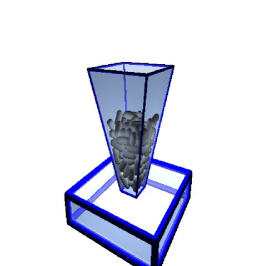
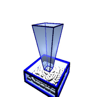
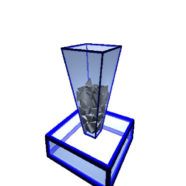
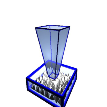
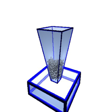
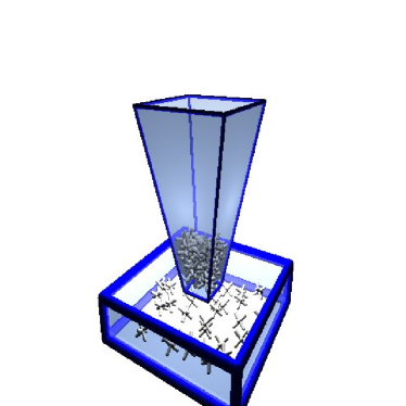
Figure 4: Hopper flow simulations at initial (left) and final (right) stages for rice (above), tetra (center) and yermis (below). The parameters are the same than in the SPC experiment. The coefficient of viscosity $\gamma$ is equal to 0.2 $s^{-1}$

Particle	$\frac{\Delta E}{E}$	$\frac{\Delta p}{p}$	$\frac{\Delta L}{L}$
rice $\Delta t=10^{-4}$	$3.6\times 10^{-3}$	$2.1\times 10^{-9}$	$2.0\times 10^{-4}$
rice $\Delta t=10^{-5}$	$4.0\times 10^{-4}$	$1.1\times 10^{-10}$	$5.8\times 10^{-5}$
tetra $\Delta t=10^{-4}$	$2.2\times 10^{-3}$	$3.2\times 10^{-9}$	$4.6\times 10^{-5}$
tetra $\Delta t=10^{-5}$	$2.0\times 10^{-4}$	$5.3\times 10^{-10}$	$1.5\times 10^{-6}$
yermis $\Delta t=10^{-4}$	$3.1\times 10^{-2}$	$1.9\times 10^{-9}$	$3.5\times 10^{-3}$
yermis $\Delta t=10^{-5}$	$2.6\times 10^{-3}$	$1.8\times 10^{-10}$	$2.3\times 10^{-4}$

Table 1: Percentage error in the numerical simulations calculated from the mechanical energy (E), angular momentum (L) and linear momentum(p) refereed to their initial values. The simulation time is 20 s, the mass of the particles is 1. kg and the stiffness is 10000 N/m

The immediate extension of the model is to include visco-elastic forces:

$$\vec{F}(G_{i},G_{j})=-k_{n}\delta(G_{i},G_{j})\vec{n}+\gamma\vec{v}_{c}$$ (7)

where $\gamma$ is the viscocity force and $\vec{v}_{c}$ is the relative velocity of the particles at the contact. This contact force offers an interesting application of this model: the study of the effect of particle shape on the jamming phenomenon of granular flow. The flow may happen when particles are discharged through a small opening, but particles may became jammed when the opening is smaller than a critical value. Modeling of gravity flow has been done using circular or spherical particles To et al. (2001), but the effect of shape on flow has not been thoughtfully investigated. In particular, non-convex particles is expected to jam more easily than convex, or circular particles.

Granular flow with convex and non-convex particles is presented using the same three particles geometries shown in Fig. 2. The simplicity of our model allow us to represent the hopper and the container as just another example of spheropolytopes, see Fig. 4. Contrary to previous findings Poeschel and Schwager (2004) our convex shaped particles do not become clogged in the hopper. This is because we have not introduced an static frictional force yet. However, as an striking result, the non-convex particles get stuck without static friction, as can be seen in Fig. 5.

Figure 5: Number of particles exiting the hopper in the setup shown in Fig 4. The simulation consider 90 particles. Note that in the yermis case the flow stops at 12 s due to clogging.

Modeling interacting particles using spheropolytopes has several advantages with respect to other existing particle-based models: i) The possibility to model non-convex particles (in our case yermis, hoppers and containers); ii) a realistic representation of the surface curvature of particles; iii) guaranteed compliance with physical laws; iv) numerical consistency, guaranteed by the continuity in the proposed contact law. v) efficiency, given by a simple model for the contact law relying only on distance calculations. This is radically different from previous approaches where the contact forces are calculated in base of overlaps Mirtich (1998); Pournin (2005)

The most interesting aspect of this model is to provide a general framework for generic particle shape and contact interactions. Spheropolytopes is a very general shape which can be uses to represent biomolecules, polymers, rocks, meteors, etc. For the modeling of geological materials, particles with random shapes and tunable roundness can be generated by applying Minkowski operators on Voronoi diagrams Galindo-Torres and Alonso-Marroquin (2008). Comminution processes can be model by solving the continuum stress equation of a given spheropolyhedra and originate from it fracture planes and hence secondary spheropolyhedra.

This work is supported by the Australian Research Council (project number DP0772409 ) and the UQ Early Carrier Research Grant.

References

- Carlson and Mccammon (2000) H. Carlson and A. Mccammon, Molecular Pharmacology 57, 213 (2000).
- Pelzl et al. (1999) G. Pelzl, S. Diele, and W. Weissflog, Advanced Materials 11, 707 (1999).
- Alonso-Marroquin et al. (2005) F. Alonso-Marroquin, S. Luding, H. Herrmann, and I. Vardoulakis, Phys. Rev. E 51, 051304 (2005).
- Mirtich (1998) B. Mirtich, ACM Transactions on Graphics (TOG) 15, 177 (1998).
- Ruspini and Khatib (2001) D. Ruspini and O. Khatib, Journal of Robotic Systems 18, 769 (2001).
- Baraff (1993) D. Baraff, Algorithmica 10, 292 (1993).
- Hasegawa and Sato (2004) S. Hasegawa and M. Sato, Computer Graphics Forum 23, 529 (2004).
- Poeschel and Schwager (2004) T. Poeschel and T. Schwager, Computational Granular Dynamics (Springer, Berlin, 2004).
- Lu and McDowell (2007) M. Lu and G. R. McDowell, Granular Matter 9, 69 (2007).
- Alonso-Marroquin (2008) F. Alonso-Marroquin, Europhysics Letters 83, 14001 (2008).
- Alonso-Marroquin and Wang (2008) F. Alonso-Marroquin and Y. Wang (2008), arXiv:0804.0474.
- Galindo-Torres and Alonso-Marroquin (2008) S. A. Galindo-Torres and F. Alonso-Marroquin (2008), submitted to Phys. Rev. E, arXiv:0811.2858v1.
- Pournin et al. (2005) L. Pournin, M. Weber, M. Tsukahara, J.-A. Ferrez, M. Ramaioli, and T. M. Liebling, Granular Matter 7, 119 (2005).
- Pournin and Liebling (2005) L. Pournin and T. Liebling, in Powders & Grains 2005 (Balkema, Leiden, 2005), pp. 1375–1478.
- Pournin (2005) L. Pournin, Ph.D. thesis, École Polytechnique Fédérale de Lausanne (2005).
- Wang et al. (2006) Y. Wang, S. Abe, S. Latham, and P. Mora, Pure and Applied Geophysics 163, 1769 (2006).
- To et al. (2001) K. To, P. Lai, and H. Pak, Physical Review Letters 86, 71 (2001).