Gauge Covariance Relations and the Fermion Propagator in Maxwell-Chern-Simons QED₃

Abstract

We study the gauge covariance of the fermion propagator in Maxwell-Chern-Simons planar quantum electrodynamics (QED₃) considering four-component spinors with parity-even and parity-odd mass terms both for fermions and photons. Starting with its tree level expression in the Landau gauge, we derive a non perturbative expression for this propagator in an arbitrary covariant gauge by means of its Landau-Khalatnikov-Fradkin transformation (LKFT). We compare our findings in the weak coupling regime with the direct one-loop calculation of the two-point Green function and observe perfect agreement up to a gauge independent term. We also reproduce results derived in earlier works as special cases of our findings.

1 Introduction

Gauge symmetry is the cornerstone of our modern understanding of fundamental interactions. At the level of field equations, such a symmetry is reflected in different relations among the Green’s functions of a given quantum field theory. In quantum electrodynamics (QED), for example, Green’s functions verify Ward-Green-Takahashi identities [1], which relate $(n+1)$-point functions with the $n$-point ones. This set of identities can be enlarged by transforming also the gauge fixing parameter $\xi$ to arrive at the Nielsen identities (NI) [2]. One advantage of these identities over the conventional Ward identities is that $\partial/\partial\xi$ becomes part of the new relations involving Green’s functions. This fact was exploited in [3] to prove the gauge independence of some physical observables related to two-point Green’s functions at the one-loop level and to all orders in perturbation theory. A different set of relations, which specify the transformation of Green’s functions under a variation of gauge, carry the name of Landau-Khalatnikov-Fradkin transformations (LKFTs) in QED, [4]. LKFTs are non perturbative in nature, and hence have the potential of playing an important role in understanding the apparent problems of gauge invariance in the strong coupling studies of Schwinger-Dyson equations (SDEs) [5]. In this context, the direct implementation of LKFTs in SDEs studies has already been reported [6, 7]. Gauge dependence studies of the SDEs must ensure that these transformation for the Green’s functions involved are satisfied [7] in order to obtain meaningful results. Rules governing LKFTs are better described in coordinate space. It is primarily for this reason that some earlier works on its implementation in the study of the fermion propagator were carried out in the coordinate space, [8]. Momentum space calculations are more demanding, owing to the complications induced by Fourier transforms. These difficulties are reflected in [9] and [10] where the non-perturbative fermion propagator was obtained starting from a perturbative one in the Landau gauge in QED in 3 and 4 space-time dimensions.

In this paper, we study QED in three space-time dimensions (QED₃) in its general form, taking into account parity conserving and violating mass terms both for photons and fermions. Specific cases of the underlying Lagrangian have found many useful applications both in condensed matter physics, particularly in high T_c-superconductivity and the quantum Hall effect [11, 12, 13, 14, 15, 16], as well as in high energy physics, mostly connected to the study of dynamical chiral symmetry breaking and confinement, where QED₃ provides a popular battleground for lattice and continuum studies [17]. An interesting review of various dynamical effects in (2+1)-dimensional theories with four-fermion interaction can be found in [18]. In all these cases, it becomes a key issue to address the gauge covariance properties of Green’s functions. We investigate the gauge structure of the fermion propagator in the light of the LKFTs. This paper is organized as follows: In the following section, considering four-component spinors, we describe the QED₃ Lagrangian with parity conserving and violating mass terms. It leads to a general fermion propagator which we write in a form suitable to study its gauge covariance relations. In section, 3 we introduce the LKFT for the fermion propagator and derive the non-perturbative expression for the two-point function under consideration. We review some limiting cases of our findings, including the massless case, the parity conserving case and the weak coupling expansion, which is compared against the one-loop calculation of the fermion propagator. It is well known that the parity violation in the fermion sector radiatively induces a Maxwell-Chern-Simons mass term for the photon. In section 4, we extend our study to include this case. At the end, we present our conclusions in section 5.

2 Fermion Propagator

As compared with its four-dimensional counterpart, only three Dirac matrices are required to describe the dynamics of planar fermions. Therefore, one can choose to work with two- or four-component spinors. Correspondingly, an irreducible or reducible representation for the $\gamma_{\mu}$-matrices would respectively be used. A discussion on the symmetries of the fermionic Lagrangian with different representations of Dirac matrices can be found in [16, 19]. In this paper, we work with four-component spinors and thus with a $4\times 4$ representation for the Dirac matrices. We choose to work in Euclidean space, where the Dirac matrices satisfy the Clifford algebra $\{\gamma_{\mu},\gamma_{\nu}\}=-2\delta_{\mu\nu}$, a realization of which is given by

$$\gamma_{0}\,\equiv\,\left(\begin{array}[]{cc}-i\sigma_{3}&0\\ 0&i\sigma_{3}\end{array}\right)\;,\qquad\gamma_{1}\,\equiv\,\left(\begin{array}[]{cc}i\sigma_{1}&0\\ 0&-i\sigma_{1}\end{array}\right)\;,\qquad\gamma_{2}\,\equiv\,\left(\begin{array}[]{cc}i\sigma_{2}&0\\ 0&-i\sigma_{2}\end{array}\right)\,,$$

and

$$\gamma_{3}\equiv\left(\begin{array}[]{cc}0&I\\ I&0\end{array}\right)\,,\qquad\gamma_{5}\equiv\gamma_{0}\gamma_{1}\gamma_{2}\gamma_{3}=\left(\begin{array}[]{cc}0&-I\\ I&\phantom{-}0\end{array}\right)\,,$$

where $\sigma_{i},\,i=1,2,3$ are the Pauli matrices and $I$ the $2\times 2$ identity matrix. Notice that once we have selected a set of matrices to write down the Dirac equation, say $\{\gamma_{0},\gamma_{1},\gamma_{2}\}$, two anti-commuting gamma matrices, namely, $\gamma_{3}$ and $\gamma_{5}$ remain unused, leading us to define two types of chiral-like transformations: $\psi\to e^{i\alpha\gamma_{3}}\psi\;$ and $\psi\to e^{i\alpha\gamma_{5}}\psi\;.$ Consequently, there exist two types of mass terms for fermions, the ordinary $m_{e}\bar{\psi}\psi$ and the $m_{o}\bar{\psi}\tau\psi\;$ with $\tau=\frac{1}{2}[\gamma_{3},\gamma_{5}]=diag(I,-I)$, sometimes referred to as the Haldane mass term. The former violates chirality, whilst the later is invariant under chiral transformations. Defining parity so that it corresponds to the inversion of only one spatial axis (preserving its discrete nature), we can represent parity transformation by ${\cal P}=-i\gamma_{5}\gamma_{1}$. We thus see that $m_{e}\bar{\psi}\psi$ is parity invariant but $m_{o}\bar{\psi}\tau\psi$ is not. This would justify the use of subscripts $e$ and $o$ for parity-even and parity-odd quantities throughout the paper. We shall be working with the Lagrangian:

$${\cal L}=\bar{\psi}(i{\not\!\partial}+e{\not\!A}-m_{e}-\tau m_{o})\psi-\frac{1}{4}F_{\mu\nu}F_{\mu\nu}-\frac{1}{2\xi}(\partial_{\mu}A_{\mu})^{2},$$ (1)

where the quantities carry their usual meaning. There are many planar condensed matter models in which the low energy sector can be written as this effective form of QED₃, for which the physical origin of the masses depends on the underlying system [11] : $d$-wave cuprate superconductors [12], $d$-density-wave states [13], layered graphite [14], including graphene in the massless version [15] and a special form of the integer quantum Hall Effect without Landau levels [16]. Chiral symmetry breaking and confinement for particular forms of this Lagrangian [17] and dynamical effects of four-fermion interactions in similar models [18] have also been considered. The inverse fermion propagator in this case takes the form

$$S_{F}^{-1}(p;\xi)=A_{e}(p;\xi){\not\!p}+A_{o}(p;\xi)\tau{\not\!p}-B_{e}(p;\xi)-B_{o}(p;\xi)\tau\;.$$ (2)

We explicitly label the propagator with the covariant gauge parameter $\xi$ as we would be interested in its expression in different gauges. The bare propagator corresponds to $A_{e}^{(0)}=1,\,A_{o}^{(0)}=0,\,B_{e}^{(0)}=m_{e},\,B_{o}^{(0)}=m_{o}$. In coordinate space, we have that

$$S_{F}^{-1}(x;\xi)=X_{e}(x;\xi){\not\!x}+X_{o}(x;\xi)\tau{\not\!x}-Y_{e}(x;\xi)-Y_{o}(x;\xi)\tau\;.$$ (3)

Rather than working with parity eigenstates, we find it convenient to work in a chiral basis. For this purpose, we introduce the chiral projectors $\chi_{\pm}=(1\pm\tau)/2$ which have the properties $\chi_{\pm}^{2}=\chi_{\pm}\;,\chi_{+}\chi_{-}=0\;,\chi_{+}+\chi_{-}=1$ . The right-handed $\psi_{+}$ and left-handed $\psi_{-}$ fermion fields are $\psi_{\pm}=\chi_{\pm}\psi$, in such a fashion that the chiral decomposition of the fermion propagator becomes

$$S_{F}(p;\xi) = -\frac{A_{+}(p;\xi){\not\!p}+B_{+}(p;\xi)}{A_{+}^{2}(p;\xi)p^{2}+B_{+}^{2}(p;\xi)}\chi_{+}-\frac{A_{-}(p;\xi){\not\!p}+B_{-}(p;\xi)}{A_{-}^{2}(p;\xi)p^{2}+B_{-}^{2}(p;\xi)}\chi_{-}$$ (4)

$$\equiv -[{\cal P}_{+}^{V}(p;\xi){\not\!p}+{\cal P}_{+}^{S}(p;\xi)]\chi_{+}-[{\cal P}_{-}^{V}(p;\xi){\not\!p}+{\cal P}_{-}^{S}(p;\xi)]\chi_{-}\;,$$

and analogously, in coordinate space

$$S_{F}(x;\xi) = -\frac{X_{+}(p;\xi){\not\!x}+Y_{+}(x;\xi)}{X_{+}^{2}(x;\xi)x^{2}+Y_{+}^{2}(x;\xi)}\chi_{+}-\frac{X_{-}(x;\xi){\not\!x}+Y_{-}(x;\xi)}{X_{-}^{2}(x;\xi)x^{2}+Y_{-}^{2}(x;\xi)}\chi_{-}$$ (5)

$$\equiv -[{\cal X}_{+}^{V}(x;\xi){\not\!x}+{\cal X}_{+}^{S}(x;\xi)]\chi_{+}-[{\cal X}_{-}^{V}(x;\xi){\not\!x}+{\cal X}_{-}^{S}(x;\xi)]\chi_{-}\;,$$

where our notation is as follows: $K_{\pm}=K_{e}\pm K_{o}$ for $K=A,B,X,Y$, while ${\cal K}^{V}$ and ${\cal K}^{S}$, for ${\cal K}={\cal P,X}$, stand for the vector and scalar parts of the right- and left- projections of the fermion propagator, respectively. Obviously, propagators (4) and (5) are related trough the Fourier transforms

$$S_{F}(p;\xi)=\int d^{3}xe^{-ip\cdot x}S_{F}(x;\xi)\;,\qquad S_{F}(x;\xi)=\int\frac{d^{3}p}{(2\pi)^{3}}e^{ip\cdot x}S_{F}(p;\xi)\;.$$ (6)

From these definitions, we are ready to study the LKFT for the fermion propagator, which we shall introduce in the next section, along with the strategy of its implementation for the study of gauge covariance of the fermion propagator.

3 LKFT and the Non Perturbative Fermion Propagator

The LKFT relating the coordinate space fermion propagator in Landau gauge to the one in an arbitrary covariant gauge in arbitrary spacetime dimensions $d$ reads :

$$S_{F}(x;\xi)=S_{F}(x;0)e^{-i[\Delta_{d}(0)-\Delta_{d}(x)]}\;,$$ (7)

where

$$\Delta_{d}(x)=-\frac{i\xi e^{2}}{16(\pi)^{d/2}}(\mu x)^{4-d}\Gamma\left(\frac{d}{2}-2\right)\;,$$ (8)

$\mu$ being a mass scale introduced for dimensional purposes. Explicitly in three dimensions, the LKFT is given by

$$S_{F}(x;\xi)=e^{-ax}S_{F}(x;0)$$ (9)

where $a=\alpha\xi/2$ and $\alpha=e^{2}/(4\pi)$ as usual. With these definitions, we are ready to study the gauge covariance of the fermion propagator from its LKFT. The strategy is as follows : (i) Start from the bare propagator in momentum space in Landau gauge and Fourier transform it to coordinate space. (ii) Apply the LKFT. (iii) Fourier transform it back to momentum space. We shall proceed to carry out this exercise below. Considering the bare propagator in Landau gauge, we have $A_{+}^{(0)}(p;0)=A_{-}^{(0)}(p;0)\ =\ 1$ and $B_{\pm}^{(0)}(p;0)=m_{e}\pm m_{o}\ \equiv\ m_{\pm}$. Therefore

$${\cal P}_{\pm}^{S\,(0)}(p;0)=\frac{m_{\pm}}{p^{2}+m_{\pm}^{2}}\;,\qquad{\cal P}_{\pm}^{V\,(0)}(p;0)=\frac{1}{p^{2}+m_{\pm}^{2}}\;.$$ (10)

Performing the Fourier transforms, we find

$${\cal X}_{\pm}^{S}(x;0)=\frac{m_{\pm}e^{-m_{\pm}x}}{4\pi x}\;,\qquad{\cal X}_{\pm}^{V}(x;0)=\frac{i(1+m_{\pm}x)e^{-m_{\pm}x}}{4\pi x^{3}}\;.$$ (11)

The LKFT is straight forward to perform. It would merely shift the argument of the exponentials in the above expressions by the amount $-ax$. Then we are only left with the inverse Fourier transform, which leads to

$${\cal P}_{\pm}^{S}(p;\xi) = \frac{m_{\pm}}{p^{2}+(a+m_{\pm})^{2}}$$

$${\cal P}_{\pm}^{V}(p;\xi) = \frac{1}{p^{2}}\Bigg{[}1-\frac{m_{\pm}(a+m_{\pm})}{p^{2}+(a+m_{\pm})^{2}}-aI(p,a+m_{\pm})\Bigg{]}\;,$$ (12)

where we have defined

$$I(p,m)=\frac{1}{p}\arctan{\left(\frac{p}{m}\right)}\;.$$ (13)

The expressions (12) yield the non perturbative form of the fermion propagator in an arbitrary covariant gauge. An important advantage of the LKFT over ordinary perturbative calculation is that the weak coupling expansion of this transformation already fixes some of the coefficients in the all order perturbative expansion of the fermion propagator (see, for example, [9, 10, 20, 21]). It is easy to show that the coefficients of the terms of the form $\alpha^{i}\xi^{i}$ get already fixed in the all order perturbative expansion of the LKFT, starting from the bare propagator, a fact that holds true in arbitrary space-time dimensions, as pointed out in [21]. Even more, if we had started with a ${\cal O}(\alpha^{n})$ propagator, all the terms of the form $\alpha^{n+i}\xi^{i}$ would already get fixed, as well as those with higher powers of $\xi$ at a given order in $\alpha$ after the perturbative expansions of the results obtained on applying the corresponding LKFT. Below we shall consider equation (12) in various limiting cases, for consistency checks.

3.1 Massless case

In the massless case, $m_{e}=m_{o}=0$, the non-perturbative fermion propagator reduces to

$${\cal P}^{S}_{\pm\,massless}(p;\xi)=0\;,\qquad{\cal P}^{V}_{\pm\,massless}(p;\xi)=\frac{1}{p^{2}}\left[1-aI(p,a)\right]\;,$$ (14)

which imply $B_{\pm}(p;\xi)=0$ and hence $B_{e}(p;\xi)=B_{o}(p;\xi)=0$, i.e, fermions remain massless in all gauges. Furthermore, $A_{+}(p;\xi)=A_{-}(p;\xi)$, such that $A_{o}(p;\xi)=0$ and

$$A_{e}(p;\xi)=\left[1-aI(p,a)\right]^{-1}\;,$$ (15)

confirming the covariant form for the massless propagator dictated by LKFT [9, 10].

3.2 Ordinary QED₃ case

The ordinary, parity-conserving case was considered in [10]. It can be derived from our results setting $m_{0}=0$, which implies $m_{\pm}=m_{e}$. Hence we straightforwardly see that ${\cal P}_{+}^{S}(p;\xi)={\cal P}_{-}^{S}(p;\xi)$ and ${\cal P}_{+}^{V}(p;\xi)={\cal P}_{-}^{V}(p;\xi)$, which in turn imply ${\cal P}^{S}_{o}(p;\xi)={\cal P}^{V}_{o}(p;\xi)=0$ and thus we only have non vanishing contribution from the even-parity part of the fermion propagator:

$${\cal P}_{e}^{S}(p;\xi) = \frac{m_{e}}{p^{2}+(a+m_{e})^{2}}$$

$${\cal P}_{e}^{V}(p;\xi) = \frac{1}{p^{2}}\Bigg{[}1-\frac{m_{e}(a+m_{e})}{p^{2}+(a+m_{e})^{2}}-aI(p,a+m_{e})\Bigg{]}\;.$$ (16)

A comparison against the results of [10] shows complete agreement in this case.

3.3 Weak Coupling Regime

Next, we take the weak coupling limit of equation (12) performing an expansion of these expressions in powers of $\alpha$, recalling that $a=\alpha\xi/2$. At ${\cal O}(\alpha)$ we find

$${\cal P}_{\pm\,weak}^{S}(p;\xi) = \frac{m_{\pm}}{p^{2}+m_{\pm}^{2}}-\frac{\alpha\xi m_{\pm}^{2}}{(p^{2}+m_{\pm}^{2})^{2}}$$

$${\cal P}_{\pm\,weak}^{V}(p;\xi) = \frac{1}{p^{2}+m_{\pm}^{2}}+\frac{\alpha\xi m_{\pm}(m_{\pm}^{2}-p^{2})}{2p^{2}(p^{2}+m_{\pm}^{2})^{2}}-\frac{\alpha\xi}{2p^{2}}I(p,m_{\pm})\;.$$ (17)

As we have pointed out earlier, the non perturbative expressions obtained from the LKFT of the fermion propagator matches onto perturbative results at the one-loop level up to a gauge independent term. In order to identify such a term, we need to calculate the one-loop perturbative result of the propagator and compare against equation (17). For this purpose it is better to work directly with the $A_{\pm}$ and $B_{\pm}$ functions, which at ${\cal O}(\alpha)$ are obtained from

$$A_{\pm}^{(1)}(p;\xi) = 1-\frac{2\pi\alpha}{p^{2}}\int\frac{d^{3}k}{(2\pi)^{3}}{\rm Tr}\Bigg{[}{\not\!p}\gamma_{\mu}S_{\pm}(k;\xi)\gamma_{\nu}\Delta_{\mu\nu}^{(0)}(q)\chi_{\pm}\Bigg{]}\;,$$

$$B_{\pm}^{(1)}(p;\xi) = m_{\pm}-2\pi\alpha\int\frac{d^{3}k}{(2\pi)^{3}}{\rm Tr}\Bigg{[}\gamma_{\mu}S_{\pm}(k;\xi)\gamma_{\nu}\Delta_{\mu\nu}^{(0)}(q)\chi_{\pm}\Bigg{]}\;,$$ (18)

where $q=k-p$ and $S_{\pm}(k;\xi)={\cal P}_{\pm}^{V\,(0)}(k;\xi){\not\!k}+{\cal P}_{\pm}^{S\,(0)}(k;\xi)$. Using the explicit form of the bare photon propagator, i.e., $\Delta_{\mu\nu}^{(0)}(q;\xi)=\left(q^{2}\delta_{\mu\nu}+(\xi-1){q_{\mu}q_{\nu}}\right)/q^{4}$, we find

$$A_{\pm}^{(1)}(p;\xi) = 1-\frac{\alpha\xi}{2\pi^{2}p^{2}}\int d^{3}k\frac{(k^{2}+p^{2})(k\cdot p)-2k^{2}p^{2}}{q^{4}(k^{2}+m_{\pm}^{2})}\;,$$

$$B_{\pm}^{(1)}(p;\xi) = m_{\pm}+\frac{\alpha(2+\xi)m_{\pm}}{2\pi^{2}}\int d^{3}k\frac{1}{q^{2}(k^{2}+m_{\pm}^{2})}\;.$$ (19)

These expressions are similar to the one-loop calculation carried out for the parity-even Lagrangian of QED₃ in [22]. The integration readily yields

$$A_{\pm}^{(1)}(p;\xi) = 1+\frac{a}{p^{2}}[m_{\pm}-(m_{\pm}^{2}-p^{2})I(p,m_{\pm})]\;,$$

$$B_{\pm}^{(1)}(p;\xi) = m_{\pm}\left[1+\alpha(\xi+2)I(p,m_{\pm})\right]\;.$$ (20)

From the above expressions we can reconstruct ${\cal P}_{\pm}^{S\,(1)}$ and ${\cal P}_{\pm}^{V\,(1)}$, finding

$${\cal P}_{\pm}^{S\,(1)}(p;\xi) = \frac{m_{\pm}}{p^{2}+m_{\pm}^{2}}-\frac{\alpha\xi m_{\pm}^{2}}{(p^{2}+m_{\pm}^{2})^{2}}+\frac{2\alpha m_{\pm}(p^{2}-m_{\pm}^{2})}{(p^{2}+m_{\pm}^{2})^{2}}I(p,m_{\pm})\;,$$

$${\cal P}_{\pm}^{V\,(1)}(p;\xi) = \frac{1}{p^{2}+m_{\pm}^{2}}+\frac{\alpha\xi m_{\pm}(m_{\pm}^{2}-p^{2})}{2p^{2}(p^{2}+m_{\pm}^{2})^{2}}-\frac{\alpha\xi}{2p^{2}}I(p,m_{\pm})$$ (21)

$$-\frac{4\alpha m_{\pm}^{2}}{p(p^{2}+m_{\pm}^{2})^{2}}\;.$$

Comparing these results against those obtained from LKFT, equation (17), we observe perfect agreement up to gauge independent terms, a difference allowed by the structure of LKFTs. Note that in the Lagrangian (1), only the term $m_{o}\bar{\psi}\tau\psi$ is parity odd. Such a term would radiatively induce a Chern-Simons term into the Lagrangian, modifying the form of the photon propagator. We study the extended Lagrangian in the following section.

4 Maxwell-Chern-Simons QED₃

The fact that the parity-odd mass term in the fermion propagator radiatively induces a parity-odd contribution into the vacuum polarization can be seen from the tensor structure of the vacuum polarization $\Pi_{\mu\nu}(q)$ at the one-loop level

$$\Pi_{\mu\nu}(q) = e^{2}\int\frac{d^{3}k}{(2\pi)^{3}}{\rm Tr}\left[\gamma_{\mu}S(k,\xi)\gamma_{\nu}S(k+q;\xi)\right]$$ (22)

$$= \left(\delta_{\mu\nu}-\frac{q_{\mu}q_{\nu}}{q^{2}}\right)\Pi^{e}(q^{2})+\epsilon_{\mu\nu\rho}q_{\rho}\Pi^{o}(q^{2})\;.$$

The second term corresponds to a Chern-Simons interaction of the form

$${\cal L}_{CS}=\frac{\theta}{4}\varepsilon_{\mu\nu\rho}A_{\mu}F_{\nu\rho}\;,$$ (23)

where $\theta=\Pi^{o}(q^{2}\to 0)$. This term is parity non invariant. Despite the fact that it is not manifestly gauge invariant, under a gauge transformation, ${\cal L}_{CS}$ changes by a total derivative (see for example [23]), rendering the corresponding action gauge invariant. The parameter $\theta$ induces a topological mass for the photons. Remarkably enough, Coleman and Hill [24] demonstrated on very general grounds that this parameter receives no contribution from two- and higher-loops. Thus, it is desirable that in the presence of the parity violating mass term for the fermions in the Lagrangian, the Chern-Simons term should be considered as well. The Maxwell-Chern-Simons QED₃ Lagrangian in this case takes the form

$${\cal L}=\bar{\psi}(i{\not\!\partial}+e{\not\!A}-m_{e}-\tau m_{o})\psi-\frac{1}{4}F_{\mu\nu}F_{\mu\nu}-\frac{1}{2\xi}(\partial_{\mu}A_{\mu})^{2}+\frac{\theta}{4}\varepsilon_{\mu\nu\rho}A_{\mu}F_{\nu\rho}.$$ (24)

This Lagrangian has been employed to describe the zero field quantum Hall effect for massive Dirac fermions [16]. In that, the gauge invariant topological mass $\theta$ is found to be related to the Hall conductivity. Whichever modification this parameter should induce in the perturbative form of the fermion propagator, it certainly will not modify the gauge dependence we found in the previous section. Thus equation (12) continues to be the same in the present case. In order to identify the role of the Chern-Simons term in the perturbative expansion of the fermion propagator, we first notice that the photon propagator associated to the Lagrangian (24) takes the form

$$\Delta_{\mu\nu}^{(0)}(q;\xi)=\frac{1}{q^{2}+\theta^{2}}\left(\delta_{\mu\nu}-\frac{q_{\mu}q_{\nu}}{q^{2}}\right)-\frac{\varepsilon_{\mu\nu\rho}q_{\rho}\theta}{q^{2}(q^{2}+\theta^{2})}+\xi\frac{q_{\mu}q_{\nu}}{q^{4}}\;.$$ (25)

Inserting this propagator into (18) and taking traces, we have

$$A_{\pm}^{(1)}(p;\xi) = 1-\frac{\alpha\xi}{2\pi^{2}p^{2}}\int d^{3}k\frac{(k^{2}+p^{2})(k\cdot p)-2k^{2}p^{2}}{q^{4}(k^{2}+m_{\pm}^{2})}$$

$$+\frac{\alpha}{\pi^{2}p^{2}}\int d^{3}k\frac{(k\cdot q)(p\cdot q)}{q^{2}(q^{2}+\theta^{2})(k^{2}+m_{\pm}^{2})}$$

$$\mp\frac{\alpha\theta m_{\pm}}{\pi^{2}p^{2}}\int d^{3}k\frac{(p\cdot q)}{q^{2}(q^{2}+\theta^{2})(k^{2}+m_{\pm}^{2})}\;,$$

$$B_{\pm}^{(1)}(p;\xi) = m_{\pm}+\frac{\alpha\xi m_{\pm}}{2\pi^{2}}\int d^{3}k\frac{1}{q^{2}(k^{2}+m_{\pm}^{2})}$$ (26)

$$+\frac{\alpha m_{\pm}}{\pi^{2}}\int d^{3}k\frac{1}{(q^{2}+\theta^{2})(k^{2}+m_{\pm}^{2})}$$

$$\mp\frac{\theta\alpha}{\pi^{2}}\int d^{3}k\frac{(k\cdot q)}{q^{2}(q^{2}+\theta^{2})(k^{2}+m_{\pm}^{2})}\;.$$

Using dimensional regularization, these integrals can be evaluated in a straightforward manner, yielding

$$A_{\pm}^{(1)}(p;\xi)\ =\ 1+\frac{\alpha}{2p^{2}\theta^{2}}\Bigg{\{}\left(\theta^{2}-p^{2}-m_{\pm}^{2}\right)\left(\theta^{2}+p^{2}+m_{\pm}^{2}\pm 2m_{\pm}\theta\right)I(p,\theta+m_{\pm})$$

$$+\left[(p^{2}+m_{\pm}^{2})(p^{2}+m_{\pm}^{2}\pm 2m_{\pm}\theta)+\xi\theta^{2}(p^{2}-m_{\pm}^{2})\right]I(p,m_{\pm})$$

$$+m_{\pm}\theta^{2}(\xi+1\mp 2)-\theta\left(p^{2}+m_{\pm}^{2}+\theta^{2}\right)\Bigg{\}}\;,$$

$$B_{\pm}^{(1)}(p;\xi)\ =\ m_{\pm}+\frac{\alpha}{\theta}\Bigg{\{}\left[2m_{\pm}\theta\pm(p^{2}+m_{\pm}^{2}+\theta^{2})\right]I(p,\theta+m_{\pm})$$

$$+\left[\xi m_{\pm}\theta\mp(p^{2}+m_{\pm}^{2})\right]I(p,m_{\pm})\pm\theta\Bigg{\}}\;.$$ (27)

Some particular limits of these expressions are considered below.

4.1 Massless photons

As $\theta\to 0$, we observe that

$$A_{\pm\ (\theta\to 0)}^{(1)}(p;\xi) = 1+\frac{a}{p^{2}}[m_{\pm}-(m_{\pm}^{2}-p^{2})I(p,m_{\pm})]$$

$$-\frac{\alpha\theta}{3p^{2}}\left(2\pm\frac{(3\mp 2)m_{\pm}^{2}}{p^{2}+m_{\pm}^{2}}+3m_{\pm}I(p,m_{\pm})\right)\;,$$

$$B_{\pm\ (\theta\to 0)}^{(1)}(p;\xi) = m_{\pm}\left[1+\alpha(\xi+2)I(p,m_{\pm})\right]$$ (28)

$$+\alpha\theta\left(-\frac{(2\mp 1)m_{\pm}}{p^{2}+m_{\pm}^{2}}\pm I(p,m_{\pm})\right).$$

A comparison against (20) reveals that we recover the “pure” QED₃ limit when photons are massless, i.e, $\theta=0$.

4.2 Massless fermions

In the absence of the Maxwell-Chern-Simons term, equation (20) reveals that if we start from massless fermions, i.e., $m_{\pm}=0$, radiative corrections, being proportional to the bare mass, do not alter their masslessness. However, for $m_{\pm}=0$ in the present case, we see from (27) that

$$B_{\pm(m_{\pm}=0)}^{(1)}(p;\xi)=\pm\frac{\alpha}{\theta}\Bigg{[}-\frac{\pi p}{2}+\theta+(p^{2}+\theta^{2})I(p,\theta)\Bigg{]}\;,$$ (29)

which readily implies $B_{e}(p;\xi)=0$, but $B_{o}(p;\xi)\propto\alpha/\theta$. This implies that even starting with massless fermions, the Maxwell-Chern-Simons term radiatively induces a parity violating mass for them. In fact, we can see that in the Landau gauge, as $\theta\to 0$, the induced mass function is,

$$m_{o}^{induced}(p;0)=\lim_{\theta\to 0}\frac{B_{\pm(m_{\pm}=0)}^{(1)}(p;0)}{A_{\pm(m_{\pm}=0)}^{(1)}(p;0)}=\frac{\alpha\theta\pi}{2p}\;,$$ (30)

and would be zero if we turn off either the interactions, i.e., $\alpha=0$, or the Maxwell-Chern-Simons mass, $\theta=0$. Such a statement, complementary to the Coleman-Hill theorem [24], was first noticed in [25], and stresses the need to include in the bare Lagrangian both the Maxwell-Chern-Simons term and the Haldane mass term simultaneously, or none at all.

4.3 Ordinary QED₃ case

The ordinary QED₃ case is recovered by setting $\theta=m_{o}=0$ in (27). This can be achieved in two steps: First, from (28) we recover the pure QED₃ results (20) by setting $\theta=0$. We then arrive at (16) by setting $m_{o}=0$ in (20), as we have previously pointed out.

4.4 Gauge dependent terms

In order to perform a comparison against the perturbative expansion of the LKFT results, equation (17), it is convenient to return to the scalar and vector parts of the propagator. We find that

$${\cal P}_{\pm}^{S}(p;\xi) = \frac{m_{\pm}}{p^{2}+m_{\pm}^{2}}-\frac{\alpha\xi m_{\pm}^{2}}{(p^{2}+m_{\pm}^{2})^{2}}$$

$$+ \frac{\alpha}{\theta^{2}(p^{2}+m_{\pm}^{2})^{2}}\Bigg{\{}\theta\left[m_{\pm}(p^{2}+m_{\pm}^{2}+\theta^{2})\pm\theta(p^{2}+(1\mp 1)m_{\pm}^{2})\right]$$

$$+ \left(p^{2}+(\theta\pm m_{\pm})^{2}\right)\Bigg{[}p^{2}(\theta\pm m_{\pm})+m_{\pm}^{2}(m_{\pm}\mp\theta)-\theta^{2}m_{\pm}\Bigg{]}$$

$$\times I(p,\theta+m_{\pm})-(p^{2}+m_{\pm}^{2})^{2}(\theta\pm m_{\pm})I(p,m_{\pm})\Bigg{\}}\;,$$

$${\cal P}_{\pm}^{V}(p;\xi) = \frac{1}{p^{2}+m_{\pm}^{2}}+\frac{\alpha\xi m_{\pm}(m_{\pm}^{2}-p^{2})}{2p^{2}(p^{2}+m_{\pm}^{2})^{2}}-\frac{\alpha\xi}{2p^{2}}I(p,m_{\pm})$$ (31)

$$+ \frac{\alpha}{2p^{2}\theta^{2}(p^{2}+m_{\pm}^{2})^{2}}\Bigg{\{}\theta\left[(p^{2}-m_{\pm}^{2})\left(p^{2}+m_{\pm}^{2}+\theta^{2}\right)\right.$$

$$\mp \left.\theta m_{\pm}\left((2\pm 1)p^{2}+(2\mp 1)m_{\pm}^{2}\right)\right]$$

$$+ \left(p^{2}+(\theta\pm m_{\pm})^{2}\right)\left[(p^{2}+m_{\pm}^{2}-\theta^{2})(p^{2}-m_{\pm}^{2})\mp 4p^{2}\theta m_{\pm}\right]$$

$$\times I(p,\theta+m_{\pm})-(p^{2}+m_{\pm}^{2})^{2}(p^{2}-m_{\pm}^{2}\mp 2\theta m_{\pm})I(p,m_{\pm})\Bigg{\}}\;.$$

The gauge dependent terms exactly match onto the LKFT results expanded in the weak coupling limit, as expected. Furthermore, the gauge independent terms, as compared to those in equation (21) exhibit a more intricate dependence on the topological parameter $\theta$. These cannot be derived from the LKFT of the tree-level fermion propagator alone.

4.5 Numerical results

In perturbation theory, higher order terms in the expansion parameter $\alpha$ are smaller than the lower order terms. Naturally, one wonders about how far would be the one-loop result as compared to the non perturbative one obtained from the LKFT in quantitative terms. In Figure 1, we have drawn the scalar and vector projections of the fermion propagator propagator in various gauges arising from: non perturbative LKF analysis, equation (12) and the one-loop perturbative treatment, equation (31). The additional gauge parameter independent terms in the one-loop results, which are absent in the weak coupling expansion of the LKFT expressions, seem to play a noticeable role in the infra red. With increasing momentum, their contribution diminishes as both the expressions in equation (12) and equation (31) start merging into each other, a statement that seems to hold true in arbitrary covariant gauges.

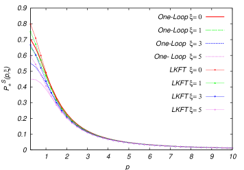
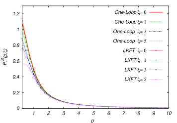
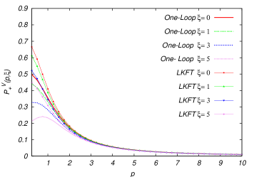
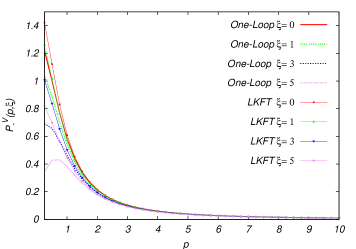
Figure 1: Scalar and vector projections of the fermion propagator in various gauges. The scale is set by the value of $e^{2}=1$ and we have chosen $m_{e}=1$, $m_{o}=0.2$ and $\theta=0.4$.

5 Conclusions

We have derived a non-perturbative expression for the fermion propagator in Maxwell-Chern-Simon QED₃ through its LKF transformation, starting from its tree level expression. Equation (12) displays one of the main results of this paper. The LKFT of the fermion propagator is written entirely in terms of basic functions of momentum, parity-even and parity-odd bare masses. Although our input is merely the bare propagator, its LKFT, being non-perturbative in nature, contains useful information of higher orders in perturbation theory. All the coefficients of the $(\alpha\xi)^{i}$ at every order are correctly reproduced without ever having to perform loop calculations. In the weak coupling regime, LKFT results match onto the one-loop perturbative results derived from the Lagrangian (1) up to gauge independent terms, a difference allowed by the structure of the LKFT. This difference arises due to our approximate input, and can be systematically removed at the cost of employing a more complex input which would need to be calculated by the brute force of perturbation theory.

Appendix

The following trace identities are fulfilled by the $\chi_{\pm}$ projectors:

$${\rm Tr}[\chi_{\pm}] = 2$$

$${\rm Tr}[\gamma^{\mu}\chi_{\pm}] = 0$$

$${\rm Tr}[\gamma^{\mu}\gamma^{\nu}\chi_{\pm}] = -2\delta^{\mu\nu}$$

$${\rm Tr}[\gamma^{\mu}\gamma^{\nu}\gamma^{\alpha}\chi_{\pm}] = \mp 2\epsilon^{\mu\nu\alpha}$$

$${\rm Tr}[\gamma^{\mu}\gamma^{\nu}\gamma^{\alpha}\gamma^{\beta}\chi_{\pm}] = 2(\delta^{\mu\nu}\delta^{\alpha\beta}-\delta^{\mu\alpha}\delta^{\nu\beta}+\delta^{\mu\beta}\delta^{\nu\alpha}).$$ (32)

References

References

• [1] J.C. Ward, Phys. Rev. 78 1 (1950); H.S. Green, Proc. Phys. Soc. (London) A66 873 (1953); Y. Takahashi, Nuovo Cimento 6 371 (1957).
• [2] N.K. Nielsen, Nucl. Phys. B101 173 (1975); O. Piguet and K. Sibold, Nucl. Phys. B253 517 (1985).
• [3] J.C. Breckenridge, M.J. Lavelle and T.G. Steele, Z. Phys. C65 155 (1995); P. Gambino and P.A. Grassi, Phys. Rev. D62 076002 (2000).
• [4] L.D. Landau and I.M. Khalatnikov, Zh. Eksp. Teor. Fiz. 29 89 (1956); L.D. Landau and I.M. Khalatnikov, Sov. Phys. JETP 2 69 (1956); E.S. Fradkin, Sov. Phys. JETP 2 361 (1956); K. Johnson and B. Zumino, Phys. Rev. Lett. 3 351 (1959); B. Zumino, J. Math. Phys. 1 1 (1960); S. Okubo, Nuovo Cim. 15 949 (1960); I. Bialynicki-Birula, Nuovo Cim. 17 951 (1960); H. Sonoda, Phys. Lett. B499 253 (2001).
• [5] F. J. Dyson, Phys. Rev. 75 1736 (1949); J. S. Schwinger, Proc. Nat. Acad. Sc. 37 452 (1951).
• [6] A. Bashir and A. Raya, Nucl. Phys. B709 307 (2005); C. S. Fischer, R. Alkofer, T. Dahm and P. Maris, Phys. Rev. D 70, 073007 (2004); Bashir A and Raya A 2006 Trends in Boson Research 1st edn, ed A V Ling (New York.: Nova Science Publishers) pp 183 229 ISBN 1-59454-521-9 (Preprint hep-ph/0411310).
• [7] A. Bashir and A. Raya, Few Body Syst. 41, 185 (2007).
• [8] R. Delbourgo and B.W. Keck, J. Phys. A13 701 (1980); R. Delbourgo, B.W. Keck and C.N. Parker, J. Phys. A14 921 (1981).
• [9] A. Bashir, Phys. Lett. B491 280 (2000)
• [10] A. Bashir and A. Raya. Phys. Rev. D66 105005 (2002).
• [11] S.G. Sharapov, V.P. Gusynin and H. Beck, Phys. Rev. B69, 075104 (2004).
• [12] N. Dorey and N.E. Mavromatos, Nucl. Phys. B386, 614 (1992); K. Farakos and N.E. Mavromatos, Mod. Phys. Lett. A13, 1019 (1998); M. Franz and Z. Tesanovic, Phys. Rev. Lett. 87, 257003 (2001); O. Vafek, A. Melikyan, M. Franz and T. Tesanovic, Phys. Rev. B63, 134509 (2001); I.F. Herbut, Phys. Rev. B66, 094504 (2002); M. Franz, Z. Tesanovic and O. Vafek, Phys. Rev. B66, 054535 (2002); M. Sutherland et. al., Phys. Rev. Lett. 94, 147004 (2005).
• [13] A.A. Nersesyan and G.E. Vachanadze, J. Low Temp Phys. 77, 293 (1989): X. Yang and C. Nayak, Phys. Rev. B65, 064523 (2002).
• [14] G.W. Semenoff, Phys. Rev. Lett. 53, 2449 (1984); J, González, F. Guinea and M.A.H. Vozmediano, Nucl. Phys. B406, 771 (1993); J, González, F. Guinea and M.A.H. Vozmediano, Phys. Rev. B63, 134421 (2001).
• [15] V.P. Gusynin and S.G. Sharapov, Phys. Rev. Lett. 95, 146801 (2005); K.S. Novoselov et. al., Nature 438, 197 (2005); Y. Zhang et. al, Nature 438, 201 (2005).
• [16] Raya A and Reyes E, 2008, J. Phys. A. 41 355401.
• [17] T. Appelquist, M.J. Bowick, D. Karabali and L.C.R. Wijewardhana, Phys. Rev. D33, 3704 (1986); M.R. Pennington and D. Walsh, Phys. Lett. B253, 246 (1991); C.J. Burden and C.D. Roberts, Phys. Rev. D44, 540 (1991); D.C. Curtis, M.R. Pennington and D. Walsh, Phys. Lett. B295, 313 (1992); K.-I. Kondo and P. Maris, Phys. Rev. D52 1212(1995); S.J. Hands, J.B. Kogut and C.G. Strouthos, Nucl. Phys. B645, 321 (2002); A. Bashir, A. Huet and A. Raya. Phys. Rev. D66, 025029 (2002); C.G. Strouthos, Nucl. Phys. Proc. Suppl. 119, 974 (2003); V.P. Gusynin and M. Reenders, Phys. Rev. D68, 025017 (2003); S.J. Hands, J.B. Kogut, L. Scorzato and C.G. Strouthos, Phys. Rev. B70, 104501 (2004); Y. Hoshino. JHEP 0409, 048 (2004); A. Bashir, A Raya, I. Clöet and C.D. Roberts, arXiv:0806.3305 [hep-ph].
• [18] A.S. Vshivtsev, B.V. Magnitsky, V.Ch. Zhukovsky, and K.G. Klimenko, Phys. Part. Nucl. 29, 523, (1998); A.S. Vshivtsev, B.V. Magnitsky, V.Ch. Zhukovsky, and K.G. Klimenko, Fiz. Elem. Chast. Atom. Yadra 29, 1259 (1998).
• [19] K. Shimizu, Prog. Theor. Phys. 74 610 (1985); Anguiano Ma de J and Bashir A, 2005 Few-Body Syst. 37 71.
• [20] A. Bashir and A. Raya, Nucl. Phys. Procc. Suppl. 141, 259 (2005).
• [21] A. Bashir and R. Delbourgo, J. Phys. A37 6587 (2004).
• [22] A. Bashir and A. Raya. Phys. Rev. D64 105001 (2001).
• [23] Khare A 2005 Fractional Statistics and Quantum Theory 2nd edn (Singapore: World Scientific) ISBN 981-256-160-9
• [24] S. Coleman and B. Hill, Phys. Lett. B159 184 (1985).
• [25] R. Delbourgo and A. Waites, Austral. J. Phys. 47, 465 (1994).