Bounds on Rayleigh-Bénard convection with general thermal boundary conditions. Part 1. Fixed Biot number boundaries

Abstract

We investigate the influence of the thermal properties of the boundaries in turbulent Rayleigh-Bénard convection on analytical bounds on convective heat transport. Using the Doering-Constantin background flow method, we systematically formulate a bounding principle on the Nusselt-Rayleigh number relationship for general mixed thermal boundary conditions of constant Biot number $\eta$ which continuously interpolates between the previously studied fixed temperature ($\eta=0$) and fixed flux ($\eta=\infty$) cases, and derive explicit asymptotic and rigorous bounds. Introducing a control parameter $R$ as a measure of the driving which is in general different from the usual Rayleigh number $\mathit{Ra}$, we find that for each $\eta>0$, as $R$ increases the bound on the Nusselt number $\mathit{Nu}$ approaches that for the fixed flux problem. Specifically, for $0<\eta\leq\infty$ and for sufficiently large $R$ ($R>R_{\mathrm{s}}={\mathcal{O}}(\eta^{-2})$ for small $\eta$) the Nusselt number is bounded as $\mathit{Nu}\leq c(\eta)R^{1/3}\leq C\mathit{Ra}^{1/2}$, where $C$ is an $\eta$-independent constant. In the $R\to\infty$ limit, the usual fixed temperature assumption is thus a singular limit of this general bounding problem.

1 Introduction

Rayleigh-Bénard convection, in which a fluid layer sandwiched between two horizontal plates is heated from below, has long attracted considerable experimental and theoretical attention; this is due not only to its importance as a model with numerous applications in engineering, geophysics, astrophysics and elsewhere, but also because it has proved such fertile ground for explorations concerning stability and dynamics, pattern formation and—under sufficient heating—convective turbulence (Cross & Hohenberg (1993); Kadanoff (2001)). Particular attention has been given to the Nusselt number $\mathit{Nu}$, representing the convective enhancement of vertical heat transport, and its dependence on the Rayleigh number $\mathit{Ra}$, a measure of the driving via the temperature difference across the fluid layer. This dependence appears to take a scaling form $\mathit{Nu}\sim f(\mathit{Pr},\Gamma)\mathit{Ra}^{p}$ (with possible logarithmic corrections), where $\Gamma$ represents geometric effects and $\mathit{Pr}$ is the Prandtl number, and a major goal of theory and experiment is to find $p$.

Observations that the heat transfer is essentially confined to thermal boundary layers near the plates, separated by an isothermal core, suggest that $p=1/3$, as proposed already by Malkus (1954); this prediction appears to be consistent with large-$\mathit{Ra}$ experiments (Niemela & Sreenivasan (2006b)) and numerical simulations of turbulent Boussinesq convection (Amati et al. (2005)). In some experiments (Chavanne et al. (1997, 2001)) an increase in the scaling exponent was observed at the highest accessible $\mathit{Ra}$ values, suggesting a possible transition to a $p=1/2$ asymptotic regime predicted by Kraichnan (1962), but other experiments at comparable $\mathit{Ra}$ have failed to observe such a transition (Glazier et al. (1999); Sommeria (1999); Niemela et al. (2000)), and possible Prandtl number variabilities or non-Boussinesq effects may have played a role (Glazier et al. (1999); Niemela & Sreenivasan (2006a, b)); strong evidence of this so-called “ultimate” regime appears to be absent.

Analytical bounds on heat transport:

While good agreement with experimentally observed scaling for a range of Rayleigh and Prandtl numbers has been attained by a phenomenological theory (Grossmann & Lohse (2001)), we focus on results derived systematically from the underlying governing differential equations. Upper bounding principles derived under some statistical assumptions, dating to the work of Howard (1963) and Busse (1969), have yielded Kraichan’s exponent $p=1/2$. More recently, Doering & Constantin (1992, 1996) realized that an idea of decomposing flow variables into “background” and “fluctuating” components, introduced by Hopf (1941) to prove energy boundedness, could be extended to obtain rigorous analytical bounds (without additional assumptions) on bulk transport quantities. The Doering-Constantin “background flow” method has since proved remarkably fruitful in obtaining bounds in good quantitative agreement with experiment or direct numerical simulation in a wide range of flows.

For Rayleigh-Bénard convection with fixed temperatures at the lower and upper boundaries of the fluid, the background flow method yields a rigorous bound $\mathit{Nu}\leq C_{0}\,\mathit{Ra}^{1/2}$ uniform in Prandtl number $\mathit{Pr}$ (Doering & Constantin (1996)), and while extensive subsequent investigations (Kerswell (1997, 2001); Plasting & Kerswell (2003)) have improved and optimized the constant $C_{0}$ in the bound, for general $\mathit{Pr}$ it has to date only proved possible to lower the exponent $p$ from the Kraichnan value $p=1/2$ under additional length scale or regularity assumptions (Constantin & Doering (1996); Kerswell (2001)). The assumption of infinite Prandtl number, however, by imposing an additional constraint on the velocity field, permits a lowering of the scaling exponent to $p=1/3$ (with possible logarithmic corrections) (Chan (1971); Constantin & Doering (1999); Ierley et al. (2006)); the best current rigorous bound in this case has the form $\mathit{Nu}\leq C(\ln\mathit{Ra})^{1/3}\mathit{Ra}^{1/3}$ (Doering et al. (2006)), and related results have recently been obtained by Wang (2008) for sufficiently large finite Prandtl number.

Influence of thermal properties of the plates:

The above analyses were performed under the usual assumption that the lower and upper boundaries of the fluid in Rayleigh-Bénard convection are held at known uniform temperature, or equivalently, that the bounding plates are perfect conductors. In practise, though, the boundaries are imperfectly conducting; and the thermal properties of the boundaries have long been understood to affect the initial instability to convection and the weakly nonlinear behaviour beyond transition (see for instance Sparrow et al. (1964); Hurle et al. (1967); Chapman & Proctor (1980); Busse & Riahi (1980) and the review in Cross & Hohenberg (1993)). Even when the bounding plates have much higher conductivity than the fluid, as the Rayleigh number (and hence the Nusselt number) increases, the effective conductivity of the fluid, depending on $\mathit{Nu}$, eventually becomes comparable to and then exceeds that of the plates; in fact, in the $\mathit{Ra}\to\infty$ limit one might expect the fluid effectively to “short circuit” the system, with the bounding plates acting essentially as perfect insulators by comparison.

The effect of the finite thermal conductivity of the bounding plates on convective heat transport has stimulated recent modelling (Chaumat et al. (2002); Chillà et al. (2004)), experimental (Brown et al. (2005)) and numerical (Verzicco (2004)) studies with the aim of reconciling various experimental results with each other and with fixed-temperature theoretical (Grossmann & Lohse (2001)) and numerical (Amati et al. (2005)) predictions. Recent numerical simulations comparing fixed flux and fixed temperature boundary conditions have reached differing conclusions: The computations of Verzicco & Sreenivasan (2008) in cylindrical geometry found $\mathit{Nu}\sim\mathit{Ra}^{1/3}$ scaling, but that for a given large enough $\mathit{Ra}$, the Nusselt number is reduced upon replacement of fixed temperature conditions at the lower boundary of the fluid by fixed flux conditions. Johnston & Doering (2007, 2008), on the other hand, found that in numerical integration of two-dimensional, horizontally periodic convection, the heat transport for large $\mathit{Ra}$ was the same, namely $\mathit{Nu}\sim\mathit{Ra}^{2/7}$, for fixed temperature and fixed flux conditions at the upper and lower boundaries of the fluid.

Predating most of the above recent investigations and with similar motivations, Otero et al. (2002) initiated the analytical study of the effects of thermal boundary conditions on Rayleigh-Bénard convection using the background flow method, obtaining a bound on the heat transport with fixed flux boundary conditions at the fluid boundaries, which again took the form $\mathit{Nu}\leq C_{\infty}\mathit{Ra}^{1/2}$ (this work was recently extended to porous medium convection by Wei (2007)). However, the mathematical structure of the fixed flux bounding problem of Otero et al. (2002), and various intermediate scaling results, turned out to be quite different from the fixed temperature case (Doering & Constantin (1996); Kerswell (2001)). It is thus natural to wonder how these two extreme cases, corresponding respectively to the idealizations of perfectly conducting and insulating plates, are related vis-à-vis their bounding problems, and which is more relevant to real, finitely conducting boundaries.

Outline of this paper:

In the present work we reconsider the effect of general thermal boundary conditions on systematically derived analytical bounds on thermal convection, continuing the program initiated by Otero et al. (2002); for simplicity we consider only identical thermal properties at the top and bottom fluid boundaries in the mathematically idealized horizontally periodic case. We consider a common model for poorly conducting plates, namely mixed (Robin) thermal boundary conditions of “Newton’s Law of Heating” type, with a fixed Biot number $\eta$, so that $\eta=0$ gives the fixed temperature and $\eta=\infty$ the fixed flux case; to our knowledge the only prior bounding study with general Biot number is the work of Siggers et al. (2004) on horizontal convection, in which mixed thermal conditions were imposed at the lower boundary of the fluid.

In Section 2 of this paper, we carefully develop a general formulation and bounding principle using the Doering-Constantin background flow method, and in Section 3 specialize to mixed thermal conditions in a manner that interpolates smoothly between the fixed temperature and fixed flux cases. The use of a piecewise linear background temperature profile and explicit estimates derived in Section 4 enables us, in Section 5, to derive analytical bounds on the $\mathit{Nu}$–$\mathit{Ra}$ relationship asymptotically valid for $\mathit{Ra}\to\infty$. For completeness, we also prove the $\mathrm{L}^{2}$ boundedness of temperature and velocity fields in Appendix A, and prove rigorous, though less sharp, bounds on the $\mathit{Nu}$–$\mathit{Ra}$ relationship in Appendix C.

Summarizing our results: Since in general the boundary temperatures are unknown a priori, it is necessary to introduce a control parameter $R$, which equals the standard Rayleigh number $\mathit{Ra}$ only in the fixed temperature case $\eta=0$. Otero et al. (2002) showed in the fixed flux case $\eta=\infty$ that while the bound was $\mathit{Nu}\leq C_{\infty}\mathit{Ra}^{1/2}$, it was obtained through the estimates $\mathit{Nu}\leq c_{1}R^{1/3}$, $\mathit{Ra}\geq c_{2}R^{2/3}$, quite unlike the fixed temperature case $\mathit{Nu}\leq C_{0}R^{1/2}$, $\mathit{Ra}=R$.

In the present work, for general sufficiently small Biot number $\eta$ we show that for small $R$ we have $\mathit{Nu}\lesssim{\mathcal{O}}(R^{1/2})$, $\mathit{Ra}\gtrsim{\mathcal{O}}(R)$ as in the fixed temperature case, but for $R$ (and hence $\mathit{Ra}$) beyond some critical parameter $R_{\mathrm{s}}={\mathcal{O}}(\eta^{-2})$, we find $\mathit{Nu}\leq c_{1}(\eta)R^{1/3}$, $\mathit{Ra}\geq c_{2}(\eta)R^{2/3}$, implying $\mathit{Nu}\leq C_{\eta}\mathit{Ra}^{1/2}$ with intermediate scaling as in the fixed flux case. Interestingly, for $\eta>0$ we find $C_{\eta}=C_{\infty}$: at least at the level of our estimates, the asymptotic scaling in each case is as for fixed flux boundary conditions (providing rigorous support for the intuition that for sufficiently high $\mathit{Ra}$, the plates essentially act as insulators), while the fixed temperature problem is a singular limit of the general asymptotic bounding problem. More details of the scaling of the bounds in different regimes, together with numerically obtained conservative bounds for piecewise linear backgrounds, will be given elsewhere (Wittenberg & Gao (2008)).

The use of mixed “Newton’s Law of Cooling” boundary conditions with fixed Biot number $\eta$ to model imperfectly conducting boundaries is a simplification, however, since in general the Biot number depends on horizontal wave number (see for instance Cross & Hohenberg (1993)). In a subsequent paper (Wittenberg (2008), Part 2 of the present work), we improve upon our model by formulating and obtaining bounds for the more realistic problem of a fluid bounded by plates of finite thickness and conductivity, establishing a systematic correspondence between that situation and the present fixed Biot number case.

2 Governing equations and bounding principle with general thermal conditions at fluid boundaries

We begin by formulating the standard Rayleigh-Bénard convection problem in the fluid and developing a bounding principle in the usual way, but without fixing the thermal conditions at the fluid boundaries. For reference and clarity, though, we occasionally point out the forms of our results in the fixed temperature and fixed flux special cases previously treated in the literature, as our development is designed to interpolate between these extremes.

2.1 Governing differential equations and nondimensionalization

In the Boussinesq approximation, the equations of motion in the fluid are

$$\frac{\partial\mathbf{u}^{*}}{\partial t^{*}}+\mathbf{u}^{*}\cdot\mbox{\boldmath$\nabla$\unboldmath}^{*}\mathbf{u}^{*}+\frac{1}{\rho_{f}}\mbox{\boldmath$\nabla$\unboldmath}^{*}P^{*} =\nu_{f}\nabla^{*2}\mathbf{u}^{*}+\alpha g(T^{*}-T_{0}){\bf e_{z}}\ ,$$ (2.1)

$$\mbox{\boldmath$\nabla$\unboldmath}^{*}\cdot\mathbf{u}^{*} =0\ ,$$ (2.2)

$$\frac{\partial T^{*}}{\partial t^{*}}+\mathbf{u}^{*}\cdot\mbox{\boldmath$\nabla$\unboldmath}^{*}T^{*} =\kappa_{f}\nabla^{*2}T^{*}\ ,$$ (2.3)

$$\mathbf{u}^{*}|_{z^{*}=0,h} =\mathbf{0}\ ,$$ (2.4)

where $\nu_{f}$ and $\kappa_{f}$ are the momentum and thermal diffusivities of the fluid, respectively, $g$ is the acceleration due to gravity, $\alpha$ is the thermal expansion coefficient, $\rho_{f}$ the fluid density at some reference temperature $T_{0}$, and $h$ is the height of the fluid layer, as in Figure 1; we also let $c_{p,f}$ be the specific heat and $\lambda_{f}=\rho_{f}\,c_{p,f}\,\kappa_{f}$ be the thermal conductivity of the fluid. In this formulation, the compressibility of the fluid is neglected everywhere except in the buoyancy force term, and the pressure is determined via the divergence-free condition on $\mathbf{u}^{*}$. Variables with an asterisk are dimensional, we have no-slip velocity boundary conditions in the vertical direction, and we take periodic boundary conditions in the horizontal directions, with periods $L^{*}_{x}$ and $L^{*}_{y}$, respectively.

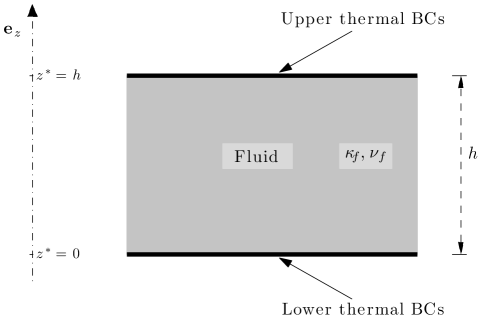
Figure 1: Geometry of Rayleigh-Bénard convection system with thermal boundary conditions imposed at upper and lower limits of fluid layer.

The present formulation is designed to be flexible with respect to the choice of thermal boundary conditions (BCs) at the plate-fluid interfaces $z^{*}=0$ and $z^{*}=h$; so in general we let $\Theta$ be a given temperature scale, determined according to the thermal BCs, and introduce a reference (“zero”) temperature $T_{\text{ref}}$.

The usual and most-studied assumption regarding thermal boundary conditions at the interfaces is that the temperature is fixed at the upper and lower boundaries:

$$T^{*}|_{z^{*}=0}\equiv T^{*}(x^{*},y^{*},0,t^{*})=T_{b}^{*},\qquad T^{*}|_{z^{*}=h}=T_{t}^{*}.$$ (2.5)

These Dirichlet BCs imply a natural choice of reference temperature $T_{\text{ref}}=T_{t}^{*}$, while the imposed temperature drop $\Delta T^{*}\equiv-\left.T^{*}\right|_{z^{*}=0}^{h}\equiv T_{b}^{*}-T_{t}^{*}$ introduces a natural temperature scale $\Theta=\Delta T^{*}$. At the opposite extreme is the fixed flux assumption that the thermal heat flux $-\lambda_{f}T^{*}_{z^{*}}\equiv-\lambda_{f}\,\partial T^{*}/\partial z^{*}$ through the fluid boundaries is a constant, which we call $\Phi$. This corresponds to the Neumann BCs of fixed normal temperature gradient $-\beta^{*}$ at the interfaces:

$$T^{*}_{z^{*}}|_{z^{*}=0}=T^{*}_{z^{*}}|_{z^{*}=h}=-\beta^{*}=-\frac{\Phi}{\lambda_{f}};$$ (2.6)

the corresponding temperature scale is $\Theta=h\beta^{*}=h\Phi/\lambda_{f}$, while in this case $T_{\text{ref}}$ is arbitrary. More general mixed (Robin) thermal BCs are discussed later in Section 3.

We nondimensionalize using $T_{\text{ref}}$ and the temperature scale $\Theta$, and with respect to the fluid layer thickness $h$ and thermal diffusivity time $h^{2}/\kappa_{f}$; that is, we take $h$, $h^{2}/\kappa_{f}$, $U=\kappa_{f}/h$ and $\rho_{f}U^{2}$ as our appropriate length, time, velocity and pressure scales respectively. For $T_{\text{ref}}\not=T_{0}$, the nondimensional fluid momentum equation will contain a constant term proportional to $T_{\text{ref}}-T_{0}$ in the ${\bf e_{z}}$ direction, which we can take care of by absorbing it into the rescaled pressure; this effect of the buoyancy force corresponds to a linear vertical pressure gradient. In summary, the nondimensional variables (without asterisks) are defined by:

$$\mathbf{x}=\frac{\mathbf{x}^{*}}{h},\quad t=\frac{t^{*}}{t_{\text{scal}}},\quad\mathbf{u}=\frac{\mathbf{u}^{*}}{U},\quad T=\frac{T^{*}-T_{\text{ref}}}{\Theta},\quad p=\frac{1}{\mathit{Pr}}\frac{P}{\rho_{f}U^{2}}-R\frac{T_{\text{ref}}-T_{0}}{\Theta}z,$$

where $t_{\text{scal}}=h^{2}/\kappa_{f}$, $U=\kappa_{f}/h$, and $\mathit{Pr}$ and $R$ are defined below. The dimensionless periodicity lengths in the transverse directions are $L_{x}=L^{*}_{x}/h$ and $L_{y}=L^{*}_{y}/h$.

The equations for the nondimensional fluid velocity $\mathbf{u}=(u,v,w)$ and fluid temperature $T$ are thus

$$\mathit{Pr}^{-1}\left(\frac{\partial\mathbf{u}}{\partial t}+\mathbf{u}\cdot\mbox{\boldmath$\nabla$\unboldmath}\mathbf{u}\right)+\mbox{\boldmath$\nabla$\unboldmath}p =\nabla^{2}\mathbf{u}+R\,T\,{\bf e_{z}},$$ (2.7)

$$\mbox{\boldmath$\nabla$\unboldmath}\cdot\mathbf{u} =0,$$ (2.8)

$$\frac{\partial T}{\partial t}+\mathbf{u}\cdot\mbox{\boldmath$\nabla$\unboldmath}T =\nabla^{2}T,$$ (2.9)

with no-slip BCs $\mathbf{u}|_{z=0,1}=\mathbf{0}$, and $L_{x},\ L_{y}$-periodic BCs in the horizontal $x$ and $y$ directions in all variables. Here the usual Prandtl number $\mathit{Pr}$ and the control parameter $R$ are defined by

$$\mathit{Pr}=\frac{\nu_{f}}{\kappa_{f}},\quad R=\frac{\alpha gh^{3}}{\nu_{f}\kappa_{f}}\Theta.$$ (2.10)

In the fixed temperature (Dirichlet) and fixed flux (Neumann) limits, the nondimensional thermal BCs are, respectively,

$$T|_{z=0}=1,\qquad T|_{z=1}=0,$$ (2.11)

$$\left.T_{z}\right|_{z=0}=\left.T_{z}\right|_{z=1}=-1.$$ (2.12)

Some additional notation:

Following Otero et al. (2002), for functions $h(x,y,z)$ and $g(t)$ we define the horizontal and time averages, $\overline{h}(z)$ and $\langle g\rangle$ respectively, by

$$\overline{h}(z)=\frac{1}{A}\iint_{A}h(x,y,z)\,dxdy=\frac{1}{A}\int_{0}^{L_{y}}\int_{0}^{L_{x}}h(x,y,z)\,dxdy$$

and

$$\langle g\rangle=\limsup_{\tau\rightarrow\infty}\frac{1}{\tau}\int_{0}^{\tau}g(t)\,dt,$$

where $A=L_{x}L_{y}$ is the nondimensional area of the plates. Also, $\int h=A\int_{0}^{1}\overline{h}(z)\,dz$ denotes a volume integral over the entire fluid layer, and the $\mathrm{L}^{2}$ norms are defined over the fluid by

$$\left\|h\right\|^{2}=\int h^{2}=\int_{0}^{1}\iint_{A}h^{2}(x,y,z)\,dxdy\,dz.$$

Finally, over the domain we consider with horizontally periodic BCs, surface integrals of vector fields $\mathbf{H}$ over the fluid boundary (the interfaces ${\mathcal{I}}$ between the plates and the fluid) are

$$\int_{{\mathcal{I}}}{\bf n}\cdot\mathbf{H}\,dS=A\left.\overline{\mathbf{H}\cdot{\bf e_{z}}}\right|_{z=0}^{1}.$$

2.2 Rayleigh and Nusselt numbers

We define the nondimensional horizontally- and time-averaged temperature drop across the fluid as

$$\Delta T=-\langle\left.\overline{T}\right|_{z=0}^{1}\rangle=\langle\overline{T}|_{z=0}-\overline{T}|_{z=1}\rangle=\frac{\Delta T^{*}}{\Theta},$$ (2.13)

where $\Delta T^{*}=\langle\overline{T^{*}}|_{z^{*}=0}-\overline{T^{*}}|_{z^{*}=h}\rangle$; we observe that this is known a priori only for fixed temperature BCs, in which case $\Delta T^{*}=T_{b}^{*}-T_{t}^{*}=\Theta$, $\Delta T=1$. The conventional Rayleigh number $\mathit{Ra}$ is defined in terms of this averaged temperature difference as

$$\mathit{Ra}=\frac{\alpha gh^{3}}{\nu_{f}\kappa_{f}}\Delta T^{*}=\frac{\alpha gh^{3}\Theta}{\nu_{f}\kappa_{f}}\Delta T,$$ (2.14)

showing that $\mathit{Ra}$ is related to the control parameter $R$ by

$$\mathit{Ra}=R\,\Delta T.$$ (2.15)

The Nusselt number $\mathit{Nu}$ is a nondimensional measure of the total heat transport through the fluid layer, which may be derived by first rewriting the thermal advection equation in the fluid (2.9) as a conservation law, $T_{t}+\mbox{\boldmath$\nabla$\unboldmath}\cdot\mathbf{J}=0$ (using incompressibility). Here the dimensionless heat current $\mathbf{J}=\mathbf{u}T+\mathbf{J}_{c}$ is composed of the conductive heat current $\mathbf{J}_{c}=-\mbox{\boldmath$\nabla$\unboldmath}T$ and the convective heat current $\mathbf{J}_{v}=\mathbf{u}T$, with corresponding overall instantaneous conductive and convective vertical heat transport $j_{c}(t)=\int{\bf e_{z}}\cdot\mathbf{J}_{c}=\iint_{A}\int_{0}^{1}-T_{z}\,dz\,dxdy=-A\left.\overline{T}\right|_{z=0}^{1}$ and $j_{v}(t)=\int{\bf e_{z}}\cdot\mathbf{J}_{v}=\int wT$, respectively. The Nusselt number $\mathit{Nu}$ is now defined as the ratio of the total (averaged) vertical heat transport, $j(t)=\int{\bf e_{z}}\cdot\mathbf{J}=j_{c}(t)+j_{v}(t)$, to the purely conductive transport:

$$\mathit{Nu}=\frac{\langle j_{c}(t)+j_{v}(t)\rangle}{\langle j_{c}(t)\rangle}=1+\frac{\frac{1}{A}\langle\int wT\rangle}{\Delta T}.$$ (2.16)

A more useful expression, which allows us to estimate $\mathit{Nu}$ from the equations of motion, is found by relating $\langle\int wT\rangle$ to the time-averaged temperature drop and boundary flux. To do so, we begin by taking the horizontal average of the temperature equation (2.9), using the horizontally periodic BCs, to get

$$\frac{\partial\overline{T}}{\partial t}+\overline{\mbox{\boldmath$\nabla$\unboldmath}\cdot\mathbf{J}}=\frac{\partial\overline{T}}{\partial t}+\frac{\partial}{\partial z}\left(\overline{wT}-\overline{T}_{z}\right)=0.$$ (2.17)

Integrating over $z$ and using the vertical no-slip boundary conditions on $w$,

$$\frac{d}{dt}{\int T}+A\int_{0}^{1}\left(\overline{wT}-\overline{T}_{z}\right)_{z}\,dz=\frac{d}{dt}{\int T}+A\left.(-\overline{T}_{z})\right|_{z=0}^{1}=0.$$ (2.18)

As we show in Appendix A, the thermal energy $\left\|T\right\|^{2}=\int T^{2}$ is uniformly bounded in time for the thermal BCs we consider, so that $\int T$ is also uniformly bounded by the Cauchy-Schwarz lemma via $\int T\leq A^{1/2}\left\|T\right\|$. Hence on taking a time average of (2.18), the time derivative term vanishes, and we find that

$$\left.\left\langle-\overline{T}_{z}\right\rangle\right|_{z=0}=\left.\left\langle-\overline{T}_{z}\right\rangle\right|_{z=1}\equiv\beta,$$ (2.19)

where the above expression defines $\beta$, the horizontally- and time-averaged vertical temperature gradient, or equivalently, the nondimensional heat flux at the fluid boundaries; note that (only) in the fixed flux case, this quantity is known, $\beta=1$. As expressed by (2.19), obviously on average, there is a balance between the heat fluxes entering the fluid layer at the bottom and leaving at the top.

Taking a time average of (2.17), via a maximum principle on $T$ the time derivative term $\langle\partial\overline{T}/\partial t\rangle$ would vanish; however, for fixed flux BCs we do not have such an a priori maximum principle. Following Otero et al. (2002), uniformly in thermal BCs we can instead multiply (2.17) by $z$ and integrate to obtain

$$\frac{d}{dt}\int_{0}^{1}z\overline{T}\,dz+\int_{0}^{1}z\left(\overline{wT}-\overline{T}_{z}\right)_{z}\,dz=0\ ;$$ (2.20)

integrating the second term by parts and using the no-slip boundary conditions, we have

$$\int_{0}^{1}z\left(\overline{wT}-\overline{T}_{z}\right)_{z}\,dz=z\left.\left(\overline{wT}-\overline{T}_{z}\right)\right|_{0}^{1}-\int_{0}^{1}\left(\overline{wT}-\overline{T}_{z}\right)\,dz=-\overline{T}_{z}|_{z=1}-\frac{1}{A}\int wT+\left.\overline{T}\right|_{z=0}^{1}.$$ (2.21)

Now as before, via

$$\int_{0}^{1}z\overline{T}\,dz=\frac{1}{A}\int zT\leq\frac{1}{A}\left(\int z^{2}\right)^{1/2}\left(\int T^{2}\right)^{1/2}=(3A)^{-1/2}\left\|T\right\|$$

and the uniform boundedness of $\left\|T\right\|$, the time average of the first term in (2.20) vanishes. Thus taking time averages of (2.20), using (2.21) and the definitions (2.13) and (2.19), we obtain

$$\frac{1}{A}\left\langle\int wT\right\rangle=\beta-\Delta T.$$ (2.22)

The expression (2.22) may now immediately be substituted into (2.16) to obtain the fundamental identity for the Nusselt number for general thermal BCs,

$$\mathit{Nu}=\frac{\beta}{\Delta T},$$ (2.23)

and consequently, using (2.15), we have $\mathit{Nu}\,\mathit{Ra}=R\,\beta$.

In the special case of fixed temperature BCs, the identity (2.23) is well-known (Doering & Constantin (1996)): with $\Delta T=1$, the Nusselt number equals the time- and horizontally-averaged flux at the boundary, $\mathit{Nu}=\beta=\langle-\overline{T}_{z}|_{z=0,1}\rangle$, and thus an upper bound on $\mathit{Nu}$ is found by bounding $\beta$ from above. For the fixed flux case, $\beta=1$ is known, the Nusselt number is the inverse of the averaged temperature drop, $\mathit{Nu}=\Delta T^{-1}$ (Otero et al. (2002)), and one seeks a lower bound on $\Delta T$. In general, though, neither $\Delta T$ nor $\beta$ is known a priori, though they are related through the thermal BCs, as discussed in Section 3.

2.3 Global energy balance

We next obtain the basic “energy” identities from the governing Boussinesq equations, which allow us to relate the Nusselt number to the momentum and heat dissipation: First, taking the inner product of the momentum equation (2.7) with $\mathbf{u}$, integrating over the fluid domain, integrating by parts and using incompressibility and no-slip BCs, we find

$$\frac{1}{2\mathit{Pr}}\frac{d}{dt}\left\|\mathbf{u}\right\|^{2}=-\left\|\mbox{\boldmath$\nabla$\unboldmath}\mathbf{u}\right\|^{2}+R\int wT.$$ (2.24)

The $\mathrm{L}^{2}$ norm of the fluid velocity is a priori bounded, as shown in Appendix A; hence, taking time averages, we derive the result (using (2.22))

$$\frac{1}{R}\langle\left\|\mbox{\boldmath$\nabla$\unboldmath}\mathbf{u}\right\|^{2}\rangle=\left\langle\int wT\right\rangle=A\left(\beta-\Delta T\right).$$ (2.25)

Observe that (2.25) implies that $\beta\geq\Delta T$, so that by (2.23) we have $\mathit{Nu}\geq 1$, as expected.

Similarly, we can take multiply the thermal advection-diffusion equation (2.9) by $T$, integrate over the fluid and integrate by parts. Neither the advection term nor the horizontal boundary terms contribute, so we find

$$\frac{1}{2}\frac{d}{dt}\left\|T\right\|^{2}=-\left\|\mbox{\boldmath$\nabla$\unboldmath}T\right\|^{2}+\int_{{\mathcal{I}}}{\bf n}\cdot(T\mbox{\boldmath$\nabla$\unboldmath}T)\,dS=-\left\|\mbox{\boldmath$\nabla$\unboldmath}T\right\|^{2}+A\left.\overline{TT_{z}}\right|_{z=0}^{1}.$$ (2.26)

Taking time averages and using boundedness of $\left\|T\right\|$, we find

$$\langle\left\|\mbox{\boldmath$\nabla$\unboldmath}T\right\|^{2}\rangle=A\left\langle\left.\overline{TT_{z}}\right|_{z=0}^{1}\right\rangle.$$ (2.27)

Again, for reference we quote these results in the known limits: for fixed temperature BCs (2.11) the global energy identities (2.25), (2.27) become (Doering & Constantin (1996))

$$\frac{1}{AR}\langle\left\|\mbox{\boldmath$\nabla$\unboldmath}\mathbf{u}\right\|^{2}\rangle =\left(\beta-1\right)=\mathit{Nu}-1,$$ (2.28)

$$\frac{1}{A}\langle\left\|\mbox{\boldmath$\nabla$\unboldmath}T\right\|^{2}\rangle =\langle-\overline{T_{z}}(0)\rangle=\beta=\mathit{Nu};$$ (2.29)

while in the fixed flux case (2.12), they are (Otero et al. (2002))

$$\frac{1}{AR}\langle\left\|\mbox{\boldmath$\nabla$\unboldmath}\mathbf{u}\right\|^{2}\rangle =\left(1-\Delta T\right)=1-\mathit{Nu}^{-1},$$ (2.30)

$$\frac{1}{A}\langle\left\|\mbox{\boldmath$\nabla$\unboldmath}T\right\|^{2}\rangle =\langle\left.-\overline{T}\right|_{z=0}^{1}\rangle=\Delta T=\mathit{Nu}^{-1}.$$ (2.31)

2.4 Background fields

In the spirit of the “background” method of Doering and Constantin, we now introduce a decomposition of the flow into a background, which carries the boundary conditions of the flow, and a space- and time-dependent fluctuating field (Doering & Constantin (1996); Kerswell (2001)). One chooses fields $\mathbf{U}$ and $\mathbf{\tau}$ which satisfy the same velocity and temperature BCs as $\mathbf{u}$ and $T$, and appropriate evolution equations—such $(\mathbf{U},\mathbf{\tau})$ are referred to as “background” flow and temperature fields—and lets $\mathbf{v}(\mathbf{x},t)$ and $\theta(\mathbf{x},t)$ be arbitrary space- and time-dependent perturbations satisfying homogeneous BCs, so that the velocity and temperature fields are decomposed into a background plus a fluctuation, according to $\mathbf{u}(\mathbf{x},t)=\mathbf{U}+\mathbf{v}(\mathbf{x},t)$, $T(\mathbf{x},t)=\mathbf{\tau}+\theta(\mathbf{x},t)$.

For simplicity of presentation we restrict our attention to the case of zero background velocity field and a $z$-dependent temperature background, $(\mathbf{U},\mathbf{\tau})=(\mathbf{0},\tau(z))$, as it appears that more general backgrounds are unlikely to improve the overall scaling of the bounds (Kerswell (2001)). Furthermore, when the upper and lower boundaries of the fluid have identical thermal properties, it is sufficient to consider only background fields satisfying $\tau^{\prime}(0)=\tau^{\prime}(1)$ (compare (2.19)), and we define

$$\Delta\tau=\tau(0)-\tau(1),\qquad\gamma=-\tau^{\prime}(0)=-\tau^{\prime}(1).$$ (2.32)

We thus define $\mathbf{v}$ and $\theta$ via the decomposition

$$\mathbf{u}(\mathbf{x},t)=\mathbf{v}(\mathbf{x},t),\qquad T(\mathbf{x},t)=\tau(z)+\theta(\mathbf{x},t),$$ (2.33)

(note that we prefer to preserve the (notational) distinction between the overall velocity field $\mathbf{u}$ and the fluctuating field $\mathbf{v}$, though for convenience we ignore this distinction in writing the components $(u,v,w)$ of the velocity field, for instance $w=\mathbf{u}\cdot{\bf e_{z}}=\mathbf{v}\cdot{\bf e_{z}}$) and immediately obtain identities between the norms of the gradients of the full solutions and their fluctuations:

$$\frac{1}{R}\left\|\mbox{\boldmath$\nabla$\unboldmath}\mathbf{u}\right\|^{2} =\frac{1}{R}\left\|\mbox{\boldmath$\nabla$\unboldmath}\mathbf{v}\right\|^{2},$$ (2.34)

$$\left\|\mbox{\boldmath$\nabla$\unboldmath}T\right\|^{2} =\left\|\mbox{\boldmath$\nabla$\unboldmath}\theta\right\|^{2}+2\int\theta_{z}\tau^{\prime}+\int\tau^{\prime 2}.$$ (2.35)

Inserting the decomposition (2.33) into the Boussinesq equations yields the evolution equations for the perturbations,

$$\mathit{Pr}^{-1}\left(\frac{\partial\mathbf{v}}{\partial t}+\mathbf{v}\cdot\mbox{\boldmath$\nabla$\unboldmath}\mathbf{v}\right)+\mbox{\boldmath$\nabla$\unboldmath}\tilde{p} =\nabla^{2}\mathbf{v}+R\,\theta\,{\bf e_{z}},$$ (2.36)

$$\mbox{\boldmath$\nabla$\unboldmath}\cdot\mathbf{v} =0,$$ (2.37)

$$\frac{\partial\theta}{\partial t}+\mathbf{v}\cdot\mbox{\boldmath$\nabla$\unboldmath}\theta =\nabla^{2}\theta+\tau^{\prime\prime}-w\tau^{\prime},$$ (2.38)

where $\mathbf{v}$ and $\theta$ satisfy appropriate homogeneous boundary conditions; that is, all fields are horizontally periodic, $\mathbf{v}$ satisfies the no-slip BCs $\mathbf{v}|_{z=0,1}=\mathbf{0}$, and $\theta$ satisfies homogeneous thermal BCs consistent with those for $T$. In particular, for fixed temperature BCs, we have $\tau(0)=1$, $\tau(1)=0$, and $\theta$ satisfies homogeneous Dirichlet BCs, $\theta|_{z=0,1}=0$; while in the fixed flux case, we require $\tau^{\prime}(0)=\tau^{\prime}(1)=-\gamma=-1$, so that $\theta$ satisfies the homogeneous Neumann BCs $\theta_{z}|_{z=0,1}=0$.

In an analogous way to the calculations of Section 2.3, we may find the energy identities for the fluctuations $\mathbf{v}$ and $\theta$: Taking the inner product of (2.36) with $\mathbf{v}$, integrating over the fluid and using incompressibility, the evolution equation for the $\mathrm{L}^{2}$ norm of the fluctuating velocity field is

$$\frac{1}{2\mathit{Pr}R}\frac{d}{dt}\left\|\mathbf{v}\right\|^{2}=-\frac{1}{R}\left\|\mbox{\boldmath$\nabla$\unboldmath}\mathbf{v}\right\|^{2}+\int w\theta,$$ (2.39)

as in (2.24). We find the corresponding $\mathrm{L}^{2}$ evolution for the perturbed temperature $\theta$ by multiplying (2.38) by $\theta$ and integrating:

$$\frac{1}{2}\frac{d}{dt}\left\|\theta\right\|^{2}=-\left\|\mbox{\boldmath$\nabla$\unboldmath}\theta\right\|^{2}+A\left.\overline{\theta\theta_{z}}\right|_{z=0}^{1}-\int\theta_{z}\tau^{\prime}+A\left.\overline{\theta}\tau^{\prime}\right|_{z=0}^{1}-\int w\theta\tau^{\prime}.$$ (2.40)

For future reference, using (2.32) and the decomposition (2.33), the second boundary term in (2.40) has time average

$$\langle\left.\overline{\theta}\tau^{\prime}\right|_{z=0}^{1}\rangle=-\gamma\langle\left.\overline{\theta}\right|_{z=0}^{1}\rangle\equiv\gamma\Delta\theta=\gamma\left(\Delta T-\Delta\tau\right).$$ (2.41)

2.5 Governing equations for general bounding principle

In order to formulate upper bounding principles for the Nusselt number, we take appropriate linear combinations of the $\mathrm{L}^{2}$ identities (2.39)–(2.40) for the fluctuating quantities, and the identities (2.34)–(2.35) for the decomposition of the gradient into background and fluctuating parts. In general, such linear combinations may contain three free parameters, over which one might optimize to obtain the best possible bound available within such a formalism (Kerswell (1997, 2001)). However, we shall consider only the restricted special case of a single “balance parameter” $b$ (Nicodemus et al. (1997)); in this simplified formulation, in fact we do not require the energy dissipation equation (2.39) at all.

We can eliminate the $\int\theta_{z}\tau^{\prime}$ term in the thermal energy equations by taking $2\cdot\eqref{eq:thL2}+\eqref{eq:gradTid}$ to give

$$\frac{1}{2}\frac{d}{dt}\left(2\left\|\theta\right\|^{2}\right)+\left\|\mbox{\boldmath$\nabla$\unboldmath}T\right\|^{2}=\int\tau^{\prime 2}-\left\|\mbox{\boldmath$\nabla$\unboldmath}\theta\right\|^{2}-2\int\theta w\tau^{\prime}+2A\left.\overline{\theta\theta_{z}}\right|_{z=0}^{1}+2A\left.\overline{\theta}\tau^{\prime}\right|_{z=0}^{1}.$$ (2.42)

Now taking a weighted average $b\cdot\eqref{eq:thbal1}+(1-b)\cdot\eqref{eq:graduid}=b\cdot[2\eqref{eq:thL2}+\eqref{eq:gradTid}]+(1-b)\cdot[0\eqref{eq:vL2}+\eqref{eq:graduid}]$, we have

$$\begin{split}\frac{1}{2}\frac{d}{dt}\left(2b\left\|\theta\right\|^{2}\right)+b\left\|\mbox{\boldmath$\nabla$\unboldmath}T\right\|^{2}+\frac{1-b}{R}\left\|\mbox{\boldmath$\nabla$\unboldmath}\mathbf{u}\right\|^{2}=b\int\tau^{\prime 2}+2bA\left.\overline{\theta}\tau^{\prime}\right|_{z=0}^{1}\\ +2bA\left.\overline{\theta\theta_{z}}\right|_{z=0}^{1}+\int\left[\frac{1-b}{R}|\mbox{\boldmath$\nabla$\unboldmath}\mathbf{v}|^{2}-2b\tau^{\prime}w\theta-b|\mbox{\boldmath$\nabla$\unboldmath}\theta|^{2}\right].\end{split}$$ (2.43)

We now take time averages and note that the time derivative term vanishes due to the boundedness of $\left\|\theta\right\|$, as shown in Appendix A. Using (2.25), (2.27) and (2.41), we find

$$bA\langle\left.\overline{TT_{z}}\right|_{z=0}^{1}\rangle+(1-b)A(\beta-\Delta T)=b\int\tau^{\prime 2}+2bA\gamma\Delta\theta+2bA\langle\left.\overline{\theta\theta_{z}}\right|_{z=0}^{1}\rangle-b\,\mathcal{Q}_{\tau,R_{\mathrm{e}}}[\mathbf{v},\theta],$$ (2.44)

where we define the quadratic form

$$\mathcal{Q}_{\tau,R_{\mathrm{e}}}[\mathbf{v},\theta]=\left\langle\int\left[\frac{b-1}{bR}|\mbox{\boldmath$\nabla$\unboldmath}\mathbf{v}|^{2}+2\tau^{\prime}w\theta+|\mbox{\boldmath$\nabla$\unboldmath}\theta|^{2}\right]\right\rangle=\left\langle\int\left[\frac{1}{R_{\mathrm{e}}}|\mbox{\boldmath$\nabla$\unboldmath}\mathbf{v}|^{2}+2\tau^{\prime}w\theta+|\mbox{\boldmath$\nabla$\unboldmath}\theta|^{2}\right]\right\rangle.$$ (2.45)

Here we have defined an “effective control parameter” $R_{\mathrm{e}}$ via

$$R_{\mathrm{e}}=\frac{b}{b-1}R,$$ (2.46)

having observed that the quadratic form $\mathcal{Q}_{\tau,R_{\mathrm{e}}}$ depends on $R$ and the balance parameter $b$ only through the combination $bR/(b-1)$. We desire a positive balance parameter $b$ so that a lower bound on $\mathcal{Q}_{\tau,R_{\mathrm{e}}}$ (and hence on $\mathcal{Q}^{\prime}_{\tau,R_{\mathrm{e}}}$ in (2.48)–(2.49) below) should imply an upper bound on $\beta$ and/or a lower bound on $\Delta T$; since a necessary condition for $\mathcal{Q}_{\tau,R_{\mathrm{e}}}$ to be a positive definite quadratic form is that $R_{\mathrm{e}}>0$ or $(b-1)/b>0$, we thus require $b>1$.

Continuing with the formulation of the governing equations, using (2.33), (2.19) and (2.32), we decompose the first term in (2.44) via

$$\langle\left.\overline{TT_{z}}\right|_{z=0}^{1}\rangle=\langle\left.\tau\overline{T_{z}}\right|_{z=0}^{1}\rangle+\langle\left.\overline{\theta}\tau^{\prime}\right|_{z=0}^{1}\rangle+\langle\left.\overline{\theta\theta_{z}}\right|_{z=0}^{1}\rangle=\beta\Delta\tau+\gamma\Delta\theta+\langle\left.\overline{\theta\theta_{z}}\right|_{z=0}^{1}\rangle.$$ (2.47)

Substituting (2.47) into (2.44), writing $\Delta\theta=\Delta T-\Delta\tau$ and rearranging terms, we obtain

$$(1-b)(\beta-\Delta T)+b\left(\beta\Delta\tau-\gamma\Delta T\right)=b\left(\int_{0}^{1}\tau^{\prime 2}\,dz-\gamma\Delta\tau\right)-\frac{b}{A}\mathcal{Q}^{\prime}_{\tau,R_{\mathrm{e}}}[\mathbf{v},\theta].$$ (2.48)

where we have now defined the quadratic form

$$\begin{split}\mathcal{Q}^{\prime}_{\tau,R_{\mathrm{e}}}[\mathbf{v},\theta]&=\mathcal{Q}_{\tau,R_{\mathrm{e}}}[\mathbf{v},\theta]-\left\langle\int_{{\mathcal{I}}}\theta{\bf n}\cdot\mbox{\boldmath$\nabla$\unboldmath}\theta\,dS\right\rangle\\ &=\left\langle\int\left[\frac{1}{R_{\mathrm{e}}}|\mbox{\boldmath$\nabla$\unboldmath}\mathbf{v}|^{2}+2\tau^{\prime}w\theta+|\mbox{\boldmath$\nabla$\unboldmath}\theta|^{2}\right]-A\left.\overline{\theta\theta_{z}}\right|_{z=0}^{1}\right\rangle.\end{split}$$ (2.49)

Equation (2.48), which is still fully independent of thermal BCs (subject to the symmetry condition $\tau^{\prime}(0)=\tau^{\prime}(1)=-\gamma$), is the governing identity underlying our upper bounding principle.

We comment that the prime in the notation $\mathcal{Q}^{\prime}_{\tau,R_{\mathrm{e}}}$ refers to the addition of the boundary terms to $\mathcal{Q}_{\tau,R_{\mathrm{e}}}$ (no implied differentiation), and note that for both fixed temperature and fixed flux BCs, the boundary term $\langle\left.\overline{\theta\theta_{z}}\right|_{z=0}^{1}\rangle$ vanishes, so $\mathcal{Q}^{\prime}_{\tau,R_{\mathrm{e}}}=\mathcal{Q}_{\tau,R_{\mathrm{e}}}$. In these cases, (2.48) thus reduces to

$$\mathit{Nu}-1=\beta-1=b\left(\int_{0}^{1}\tau^{\prime 2}\,dz-1\right)-\frac{b}{A}\mathcal{Q}_{\tau,R_{\mathrm{e}}}[\mathbf{v},\theta]$$ (2.50)

for Dirichlet thermal BCs (for which $\Delta T=\Delta\tau=1$), and to

$$1-\mathit{Nu}^{-1}=1-\Delta T=b\left(\int_{0}^{1}\tau^{\prime 2}\,dz-2\Delta\tau+1\right)-\frac{b}{A}\mathcal{Q}_{\tau,R_{\mathrm{e}}}[\mathbf{v},\theta].$$ (2.51)

for Neumann thermal BCs, in which case $\beta=\gamma=1$. For general thermal BCs, $\beta$ and $\Delta T$ are both a priori unknown, but they are related via the boundary conditions (see for instance (3.5) below), so that (2.48) may be written in terms only of either $\beta$ or $\Delta T$.

2.6 Allowed fields, admissible backgrounds and the spectral constraint

As formulated thus far, the general governing equation (2.48) is an identity. If, for given thermal BCs, one had access to $\mathbf{v}(\mathbf{x},t)$ and $\theta(\mathbf{x},t)$ satisfying (2.36)–(2.38), or sufficient information about them to compute the time-averaged quadratic form $\mathcal{Q}^{\prime}_{\tau,R_{\mathrm{e}}}[\mathbf{v},\theta]$ (2.49), then $\beta$ and $\Delta T$, and hence $\mathit{Nu}$, could in principle be computed. However, for turbulent convection such analytical information is well beyond the limits of what is (currently) accessible. The fundamental insight underlying upper bounding methods for convection is firstly, that if for some $\tau$ and $b$, $\mathcal{Q}^{\prime}_{\tau,R_{\mathrm{e}}}$ can be shown to be bounded below, then this yields, ultimately, an upper bound on the Nusselt number $\mathit{Nu}$ (for a given $R$); and secondly, that such a lower bound on $\mathcal{Q}^{\prime}_{\tau,R_{\mathrm{e}}}$ may indeed often be demonstrated provided one is prepared to widen the class of fields $\mathbf{v}$, $\theta$ over which the minimization takes place, as long as this class contains all solutions of (2.36)–(2.38). The cost of weakening the constraints on $\mathbf{v}$ and $\theta$ is that this may reduce the lower bound on $\mathcal{Q}^{\prime}_{\tau,R_{\mathrm{e}}}$ and thereby weaken the upper bound estimate for $\mathit{Nu}$.

Allowed fields $\mathbf{v}$, $\theta$:

In considering the class of allowable flows $\mathbf{v}=\mathbf{u}$ and (fluctuation) temperature fields $\theta=T-\tau$ over which to minimize $\mathcal{Q}^{\prime}_{\tau,R_{\mathrm{e}}}$, we observe that if the dynamical constraints (2.36)–(2.38) on the fields $[\mathbf{v},\theta]$ are removed without being replaced by assumptions on the temporal structure or correlations of the fields—detailed knowledge of which is unavailable—it becomes sufficient to minimize the quadratic form $\mathcal{Q}^{\prime}_{\tau,R_{\mathrm{e}}}$ over stationary fields $\mathbf{v}(\mathbf{x})$ and $\theta(\mathbf{x})$. The conditions we can assume these fields $\mathbf{v}(\mathbf{x})$ and $\theta(\mathbf{x})$ to satisfy are: appropriate homogeneous boundary conditions, the incompressibility constraint on the velocity fluctuations, and boundedness of $\left\|\mathbf{v}\right\|$ and $\left\|\theta\right\|$ (see Appendix A). More precisely, we denote the “allowed” fields $\mathbf{v}$ and $\theta$ over which we minimize $\mathcal{Q}^{\prime}_{\tau,R_{\mathrm{e}}}$ to be defined on $[0,L_{x}]\times[0,L_{y}]\times[0,1]$, periodic in the horizontal directions, so that $\mbox{\boldmath$\nabla$\unboldmath}\cdot\mathbf{v}=0$, $\mathbf{v}=\mathbf{0}$ on $z=0,1$, and $\theta$ satisfies homogeneous thermal boundary conditions consistent with those of $T$. For fixed temperature convection, plausible but non-rigorous regularity assumptions restricting the class of allowed fields have been shown to improve the scaling of the $\mathit{Nu}$-$\mathit{Ra}$ bounds (Constantin & Doering (1996); Kerswell (2001)), but we shall not pursue such assumptions here.

Observe that according to the above description, the trivial fields $\mathbf{v}=\mathbf{0}$, $\theta=0$ are “allowed”, though they do not satisfy (2.36)–(2.38) for $\tau^{\prime\prime}\not=0$. Since furthermore, $\mathcal{Q}^{\prime}_{\tau,R_{\mathrm{e}}}[\lambda\mathbf{v},\lambda\theta]=\lambda^{2}\mathcal{Q}^{\prime}_{\tau,R_{\mathrm{e}}}[\mathbf{v},\theta]$ for $\lambda\in\mathbb{R}$, it follows that if $\mathcal{Q}^{\prime}_{\tau,R_{\mathrm{e}}}$ is bounded below, then the minimum is zero.

Admissible backgrounds:

For each $R_{\mathrm{e}}>0$ (that is, for each $R>0$ and $b>1$), we thus denote a background field $\tau(z)$ admissible if it satisfies the appropriate BCs, the same as those for $T$ at the upper and lower interfaces; and if the resultant quadratic form $\mathcal{Q}^{\prime}_{\tau,R_{\mathrm{e}}}$ is non-negative, $\mathcal{Q}^{\prime}_{\tau,R_{\mathrm{e}}}[\mathbf{v},\theta]\geq 0$ for all allowed fields $\mathbf{v}$ and $\theta$.

Note that the positivity condition on the quadratic form $\mathcal{Q}^{\prime}_{\tau,R_{\mathrm{e}}}[\mathbf{v},\theta]\geq 0$ is equivalent to

$$\Lambda(\tau,R_{\mathrm{e}})=\mathop{\inf_{\mathbf{v},\theta}}_{\left\|\mathbf{v}\right\|^{2}+\left\|\theta\right\|^{2}\not=0}\left(\frac{\mathcal{Q}^{\prime}_{\tau,R_{\mathrm{e}}}[\mathbf{v},\theta]}{\left\|\mathbf{v}\right\|^{2}+\left\|\theta\right\|^{2}}\right)\geq 0,$$ (2.52)

where the infimum is taken over allowed fields $\mathbf{v}$ and $\theta$. Via the associated Euler-Lagrange equations, the condition (2.52) is equivalent to requiring that the linear operator

$$\mathcal{L}_{\tau,R_{\mathrm{e}}}\begin{pmatrix}\mathbf{v}\\ \theta\end{pmatrix}=\begin{pmatrix}-\frac{1}{R_{\mathrm{e}}}\nabla^{2}\mathbf{v}+\tau^{\prime}\theta+\mbox{\boldmath$\nabla$\unboldmath}p\\ -\nabla^{2}\theta+\tau^{\prime}w\end{pmatrix}$$ (2.53)

acting on allowed fields $\mathbf{v}$, $\theta$ has a positive semi-definite spectrum, or that the lowest eigenvalue $\Lambda_{0}$ of $\mathcal{L}_{\tau,R_{\mathrm{e}}}$ is non-negative. Consequently, the admissibility criterion on background fields $\tau(z)$ (for a given $R_{\mathrm{e}}=bR/(b-1)>0$), equivalent to (2.52), is also referred to as a spectral constraint on $\tau$ (Doering & Constantin (1996)).

Fourier formulation of admissibility condition:

Due to the horizontal periodicity of the problem, we may reformulate the admissibility condition $\mathcal{Q}^{\prime}_{\tau,R_{\mathrm{e}}}\geq 0$ in horizontally Fourier-transformed variables: we write the vertical component of velocity $w$ and temperature fluctuation $\theta$ as

$$w(x,y,z)=\sum_{\mathbf{k}}\mathrm{e}^{{\mathrm{i}}(k_{x}x+k_{y}y)}\hat{w}_{\mathbf{k}}(z),\qquad\theta(x,y,z)=\sum_{\mathbf{k}}\mathrm{e}^{{\mathrm{i}}(k_{x}x+k_{y}y)}\hat{\theta}_{\mathbf{k}}(z),$$ (2.54)

where the horizontal wave vector is $\mathbf{k}=(k_{x},k_{y})=(2\pi n_{x}/L_{x},2\pi n_{y}/L_{y})$, and we write $k^{2}=|\mathbf{k}|^{2}$; we shall also write ${\hat{w}_{\mathbf{k}}}^{*}$ for the complex conjugate of $\hat{w}_{\mathbf{k}}$ and $\mathrm{D}=d/dz$. We can use incompressibility to express the transformed horizontal components of velocity in terms of the vertical component, so that the admissibility criterion may be written completely in terms of the Fourier modes $\hat{w}_{\mathbf{k}}$ and $\hat{\theta}_{\mathbf{k}}$. This considerably simplifies the formulation, particularly since $\mathcal{Q}^{\prime}_{\tau,R_{\mathrm{e}}}$ is a quadratic form (equivalently, the Euler-Lagrange equations for the minimization problem are linear), so that different horizontal Fourier modes decouple. The no-slip boundary condition and incompressibility imply that the BCs for $\hat{w}_{\mathbf{k}}(z)$ are $\hat{w}_{\mathbf{k}}=\mathrm{D}\hat{w}_{\mathbf{k}}=0$ for $z=0,1$; the BCs on $\hat{\theta}_{\mathbf{k}}$ obviously depend on the choice of thermal BCs, which have so far been left unspecified. We note also that $\hat{w}_{\mathbf{0}}=0$; this follows from incompressibility and horizontal periodicity via $A\,\partial\overline{w}/\partial z=\iint_{A}w_{z}\,dx\,dy=-\iint_{A}(u_{x}+v_{y})\,dx\,dy=0$, which implies using $\overline{w}|_{z=0}=0$ that $\overline{w}=0$ for all $z$.

Substituting (2.54) into (2.45) and using incompressibility, as in Otero et al. (2002) we can write the quadratic form $\mathcal{Q}_{\tau,R_{\mathrm{e}}}$ evaluated on allowed (stationary) fields $\mathbf{v}$ and $\theta$ as

$$\mathcal{Q}_{\tau,R_{\mathrm{e}}}[\mathbf{v},\theta]=\int\left[\frac{1}{R_{\mathrm{e}}}|\mbox{\boldmath$\nabla$\unboldmath}\mathbf{v}|^{2}+2\tau^{\prime}w\theta+|\mbox{\boldmath$\nabla$\unboldmath}\theta|^{2}\right]\geq A\sum_{\mathbf{k}}\mathcal{Q}_{\mathbf{k}},$$ (2.55)

where (see Constantin & Doering (1996); Kerswell (2001))

$$\mathcal{Q}_{\mathbf{k}}\equiv\mathcal{Q}_{\mathbf{k};\tau,R_{\mathrm{e}}}[\hat{w}_{\mathbf{k}},\hat{\theta}_{\mathbf{k}}] =\int_{0}^{1}\left[\frac{1}{R_{\mathrm{e}}}\left(k^{2}|\hat{w}_{\mathbf{k}}|^{2}+2|\mathrm{D}\hat{w}_{\mathbf{k}}|^{2}+\frac{1}{k^{2}}|\mathrm{D}^{2}\hat{w}_{\mathbf{k}}|^{2}\right)+2\tau^{\prime}\text{Re}[\hat{w}_{\mathbf{k}}{\hat{\theta}_{\mathbf{k}}}^{*}]\right.$$

$$\qquad\quad\ \left.+\left(k^{2}|\hat{\theta}_{\mathbf{k}}|^{2}+|\mathrm{D}\hat{\theta}_{\mathbf{k}}|^{2}\right)\right]\,dz\ ;$$ (2.56)

note that (2.55) is an equality for two-dimensional flows. Since the boundary terms in (2.49) are expressed in Fourier space as $\left.\overline{\theta\theta_{z}}\right|_{z=0}^{1}=\sum_{\mathbf{k}}\left.\text{Re}[\hat{\theta}_{\mathbf{k}}(z)\,\mathrm{D}{\hat{\theta}_{\mathbf{k}}}^{*}(z)]\right|_{z=0}^{1}$, we thus define

$$\mathcal{Q}^{\prime}_{\mathbf{k}}\equiv\mathcal{Q}^{\prime}_{\mathbf{k};\tau,R_{\mathrm{e}}}[\hat{w}_{\mathbf{k}},\hat{\theta}_{\mathbf{k}}]=\mathcal{Q}_{\mathbf{k}}-\left.\text{Re}[\hat{\theta}_{\mathbf{k}}(z)\,\mathrm{D}{\hat{\theta}_{\mathbf{k}}}^{*}(z)]\right|_{z=0}^{1},$$ (2.57)

to give

$$\mathcal{Q}^{\prime}_{\tau,R_{\mathrm{e}}}[\mathbf{v},\theta]=\int\left[\frac{1}{R_{\mathrm{e}}}|\mbox{\boldmath$\nabla$\unboldmath}\mathbf{v}|^{2}+2\tau^{\prime}w\theta+|\mbox{\boldmath$\nabla$\unboldmath}\theta|^{2}\right]-A\left.\overline{\theta\theta_{z}}\right|_{z=0}^{1}\geq A\sum_{\mathbf{k}}\mathcal{Q}^{\prime}_{\mathbf{k}}.$$ (2.58)

Since the class of allowed fields $[\mathbf{v},\theta]$ includes fields containing a single horizontal Fourier mode, it is now clear that $\mathcal{Q}^{\prime}_{\tau,R_{\mathrm{e}}}$ is a positive quadratic form, $\mathcal{Q}^{\prime}_{\tau,R_{\mathrm{e}}}[\mathbf{v},\theta]\geq 0$ for all allowed fields $\mathbf{v}$ and $\theta$, if and only if all the quadratic forms $\mathcal{Q}^{\prime}_{\mathbf{k}}=\mathcal{Q}^{\prime}_{\mathbf{k};\tau,R_{\mathrm{e}}}$ are positive. Thus the admissibility criterion for background fields $\tau(z)$ (for given $R_{\mathrm{e}}>0$) may be formulated in Fourier space, as the condition that $\mathcal{Q}^{\prime}_{\mathbf{k}}[\hat{w}_{\mathbf{k}},\hat{\theta}_{\mathbf{k}}]\geq 0$ for all $\mathbf{k}$ and for all sufficiently smooth (complex-valued) functions $\hat{w}_{\mathbf{k}}(z)$, $\hat{\theta}_{\mathbf{k}}(z)$ satisfying $\hat{w}_{\mathbf{k}}=\mathrm{D}\hat{w}_{\mathbf{k}}=0$ at $z=0,1$ and the appropriate boundary conditions on $\hat{\theta}_{\mathbf{k}}$ at $z=0,1$.

Bounding principle:

The thermal BCs at the plates imply an equation relating $\beta$ and $\Delta T$, whenever they do not specify either $\Delta T$ (fixed temperature) or $\beta$ (fixed flux) directly. Thus, for instance (for BCs other than fixed flux), we can substitute for $\Delta T$ and write (2.48) in terms of only $\beta$, as done below (the fixed temperature and fixed flux cases are given in (2.50)–(2.51)).

In such a case for a given $R$ and $b$, for any admissible background field $\tau(z)$ the inequality $\mathcal{Q}^{\prime}_{\tau,R_{\mathrm{e}}}\geq 0$ implies an upper bound $\mathcal{B}[\tau;b]$ on the averaged boundary flux $\beta$. Via the relation between $\beta$ and $\Delta T$, this also gives a lower bound $\mathcal{D}[\tau;b]$ on the averaged temperature drop across the fluid; using (2.23), in this way admissible backgrounds lead to upper bounds $\mathcal{N}[\tau;b]$ for $\mathit{Nu}$. For a given $R>0$, the best upper bound $\tilde{\mathcal{N}}(R)$ on $\mathit{Nu}$ obtainable using this approach is now obtained by minimizing $\mathcal{N}[\tau;b]$ over admissible $\tau(z)$ and $b$. Finally, the relationship $\mathit{Ra}=R\,\Delta T\geq R\,\mathcal{D}[\tau;b]$ lets us bound $R$, and hence $\mathit{Nu}$, from above as a function of $\mathit{Ra}$.

3 Mixed (Robin) thermal boundary conditions

The formulation and derivations above were developed independent of thermal boundary conditions, except that we have restricted our attention to fluids with thermally identical upper and lower boundaries, which permits the symmetry assumption $\tau^{\prime}(0)=\tau^{\prime}(1)=-\gamma$. We now specialize to particular BCs to make further progress: General linear conditions at the boundary of a fluid as in figure 1 are of mixed (Robin) type. In a subsequent paper we consider the more realistic case of a fluid in thermal contact with bounding plates of finite thickness and conductivity.

3.1 Fixed Biot number boundary conditions and nondimensionalization

In dimensional terms, we choose the mixed (Robin) BCs on the plates to take the form

$$T^{*}+\eta^{*}{\bf n}\cdot\mbox{\boldmath$\nabla$\unboldmath}^{*}T^{*}=A_{l}^{*}\ \ \text{on}\ \ z^{*}=0,\qquad T^{*}+\eta^{*}{\bf n}\cdot\mbox{\boldmath$\nabla$\unboldmath}^{*}T^{*}=A_{u}^{*}\ \ \text{on}\ \ z^{*}=h.$$ (3.1)

for some given constant $0\leq\eta^{*}<\infty$. These conditions may be interpreted as Newton’s Law of Cooling (Heating), in which the boundary heat flux is assumed proportional to the temperature change across the boundary: $-\lambda_{f}{\bf n}\cdot\mbox{\boldmath$\nabla$\unboldmath}^{*}T^{*}=\lambda_{f}(T^{*}-A_{l}^{*})/\eta^{*}$.

We use ${\bf n}=-{\bf e_{z}},+{\bf e_{z}}$ on $z^{*}=0,h$ respectively, and nondimensionalize by substituting $z^{*}=hz$, $T^{*}=T_{\text{ref}}+\Theta T$. Defining the Biot number $\eta=\eta^{*}/h$, we find

$$T-\eta\,T_{z}=\frac{A_{l}^{*}-T_{\text{ref}}}{\Theta}\ \ \text{on}\ \ z=0,\qquad T+\eta\,T_{z}=\frac{A_{u}^{*}-T_{\text{ref}}}{\Theta}\ \ \text{on}\ \ z=1.$$ (3.2)

At the moment $T_{\text{ref}}$ and $\Theta$ are still unspecified. A convenient choice, consistent with the nondimensionalizations introduced previously for the limiting fixed temperature and fixed flux cases, is to require the conducting state ($\mathbf{u}^{*}=\mathbf{0}$, $\mbox{\boldmath$\nabla$\unboldmath}^{*}T^{*}=C\,{\bf e_{z}}$ for some constant $C<0$) to take the form $\mathbf{u}=\mathbf{0}$, $T=1-z$ in the nondimensional variables. The condition that $T=1-z$ satisfies the nondimensional BCs (3.2) implies $(A_{l}^{*}-T_{\text{ref}})/\Theta=1+\eta$, $(A_{u}^{*}-T_{\text{ref}})/\Theta=-\eta$, so that (for $\eta<\infty$) our chosen temperature scale and reference temperature are

$$\Theta=\frac{A_{l}^{*}-A_{u}^{*}}{1+2\eta},\qquad T_{\text{ref}}=\frac{A_{u}^{*}+\eta(A_{l}^{*}+A_{u}^{*})}{1+2\eta}.$$ (3.3)

Having finally fixed a choice of dimensionless variables, the nondimensional mixed thermal boundary conditions (fixed Biot number) are

$$T-\eta\,T_{z}=1+\eta\ \ \text{on}\ \ z=0,\qquad T+\eta\,T_{z}=-\eta\ \ \text{on}\ \ z=1.$$ (3.4)

Note that the mixed (Robin) BCs (3.4) reduce to the fixed temperature (Dirichlet) BCs (2.11) in the limit $\eta\to 0$, and to the fixed flux (Neumann) BCs (2.12) in the limit $\eta\to\infty$; thus we denote $\eta=0$ and $\eta=\infty$ as the “fixed temperature” and “fixed flux” cases, respectively.

3.2 Governing identities for fixed finite Biot number

In the general case, neither the boundary temperature drop $\Delta T$ nor the flux $\beta$ that combine in the computation (2.23) of the Nusselt number is known a priori. However, we can derive a relation between them: taking horizontal averages of (3.4), and subtracting the upper boundary condition from the lower, we find $\overline{T}|_{z=0}-\overline{T}|_{z=1}-\eta(\overline{T}_{z}|_{z=0}+\overline{T}_{z}|_{z=1})=1+2\eta$. Taking time averages and using (2.13) and (2.19), we find the fundamental relation

$$\Delta T+2\eta\beta=1+2\eta$$ (3.5)

(this formula also holds in the fixed temperature and flux limits $\eta\rightarrow 0$ and $\eta\rightarrow\infty$). Hence for $0<\eta<\infty$, an upper bound on $\beta$ constitutes a lower bound on $\Delta T$, and vice versa, and we only need to bound one of these quantities to obtain an upper bound on $\mathit{Nu}=\beta/\Delta T=\beta/[1+2\eta(1-\beta)]=\Delta T^{-1}+\left(\Delta T^{-1}-1\right)/2\eta$.

Using the identity (3.5) to solve for either $\Delta T=1+2\eta(1-\beta)$ or $\beta=1+(1-\Delta T)/2\eta$ and substituting into the results of Sections 2.3–2.5, we obtain the forms of the governing energy identities for mixed thermal BCs. We shall state these identities in a way that permits us to obtain an upper bound on $\beta$ (the relations are stated in terms of $\beta$, $\gamma$, $\langle\overline{T_{z}^{2}}|_{z=0,1}\rangle$ and $\langle\overline{\theta_{z}^{2}}|_{z=0,1}\rangle$, valid for $\eta<\infty$); this is the formulation suitable for small $\eta$, which reduces to the corresponding previously stated identities for fixed temperature BCs in the limit $\eta\to 0$. For completeness, in Appendix B we give the forms of the identities (equivalent for $0<\eta<\infty$) which yield the fixed flux limit $\eta\to\infty$.

First, solving for $\Delta T$ from (3.5) and substituting into the global kinetic energy identity (2.25), we find

$$\frac{1}{AR}\langle\left\|\mbox{\boldmath$\nabla$\unboldmath}\mathbf{u}\right\|^{2}\rangle=\beta-\Delta T=(1+2\eta)\left(\beta-1\right)$$ (3.6)

which reduces to (2.28) in the limit $\eta\rightarrow 0$. Similarly, we can evaluate the boundary term in (2.27) by using the BCs (3.4) to solve for $T$ at $z=0,1$ in terms of $T_{z}$; substituting into $\left.TT_{z}\right|_{z=0}^{1}$ and taking horizontal and time averages, we find that the global thermal energy identity (2.27) becomes

$$\frac{1}{A}\langle\left\|\mbox{\boldmath$\nabla$\unboldmath}T\right\|^{2}\rangle=\langle\left.\overline{TT_{z}}\right|_{z=0}^{1}\rangle=(1+2\eta)\beta-\eta\langle\overline{T_{z}^{2}}|_{z=0}+\overline{T_{z}^{2}}|_{z=1}\rangle$$ (3.7)

which again reduces to the appropriate fixed temperature limit (2.29).

In the background flow formulation, the requirement for the background field to satisfy the given BCs in this case means that $\tau(z)$ should obey (3.4), implying that

$$\Delta\tau+2\eta\gamma=1+2\eta$$ (3.8)

using (2.32). Consequently, the perturbation $\theta$ satisfies the homogeneous Robin BCs $\theta+\eta{\bf n}\cdot\mbox{\boldmath$\nabla$\unboldmath}\theta=0$ at the interfaces, which in our geometry become

$$\theta-\eta\,\theta_{z}=0\ \ \text{at}\ \ z=0,\qquad\theta+\eta\,\theta_{z}=0\ \ \text{at}\ \ z=1,$$ (3.9)

and translate for horizontal Fourier modes defined in (2.54) to the BCs

$$\hat{\theta}_{\mathbf{k}}(0)=\eta\,\mathrm{D}\hat{\theta}_{\mathbf{k}}(0),\qquad\hat{\theta}_{\mathbf{k}}(1)=-\eta\,\mathrm{D}\hat{\theta}_{\mathbf{k}}(1).$$ (3.10)

The boundary term in (2.49) is thus $\int_{{\mathcal{I}}}\theta\,{\bf n}\cdot\mbox{\boldmath$\nabla$\unboldmath}\theta\,dS=-\eta\int_{{\mathcal{I}}}({\bf n}\cdot\mbox{\boldmath$\nabla$\unboldmath}\theta)^{2}\,dS\leq 0$, or

$$\left.\overline{\theta\theta_{z}}\right|_{z=0}^{1}=-\eta(\overline{\theta_{z}^{2}}|_{z=0}+\overline{\theta_{z}^{2}}|_{z=1}),$$ (3.11)

which can equivalently be written in Fourier space (see (2.57)) as

$$\left.\overline{\theta\theta_{z}}\right|_{z=0}^{1}=\sum_{\mathbf{k}}\left.\text{Re}[\hat{\theta}_{\mathbf{k}}(z)\mathrm{D}{\hat{\theta}_{\mathbf{k}}}^{*}(z)]\right|_{z=0}^{1}=-\eta\sum_{\mathbf{k}}\left(|\mathrm{D}\hat{\theta}_{\mathbf{k}}(0)|^{2}+|\mathrm{D}\hat{\theta}_{\mathbf{k}}(1)|^{2}\right).$$ (3.12)

It follows that $\mathcal{Q}^{\prime}_{\tau,R_{\mathrm{e}}}[\mathbf{v},\theta]\geq\mathcal{Q}_{\tau,R_{\mathrm{e}}}[\mathbf{v},\theta]$, so that a lower bound on $\mathcal{Q}_{\tau,R_{\mathrm{e}}}$ implies a lower bound on $\mathcal{Q}^{\prime}_{\tau,R_{\mathrm{e}}}$; the additional boundary term which appears for $\eta\not=0,\infty$ is stabilizing.

Finally, the form of the governing identity (2.48) for mixed thermal BCs, fundamental to the formulation of a bounding principle, may now be derived: Solving and substituting for $\Delta T$ and $\Delta\tau$ using (3.5) and (3.8), we find

$$\beta\Delta\tau-\gamma\Delta T+\gamma\Delta\tau=(1+2\eta)\beta-2\eta\gamma^{2}.$$ (3.13)

Now substituting (3.6) and (3.13), (2.48) becomes in terms of $\beta$ (compare (2.50))

$$(1+2\eta)(\beta-1)=b\left(\int_{0}^{1}\tau^{\prime 2}\,dz-(1+2\eta)+2\eta\gamma^{2}\right)-\frac{b}{A}\mathcal{Q}^{\prime}_{\tau,R_{\mathrm{e}}}[\mathbf{v},\theta],$$ (3.14)

where we evaluate the boundary term in $\mathcal{Q}^{\prime}_{\tau,R_{\mathrm{e}}}[\mathbf{v},\theta]$ using (3.11).

3.3 A bounding principle for mixed thermal boundary conditions

Following the general approach outlined in Section 2.6, the governing equations derived in Section 3.2 now allow us to formulate an upper bounding principle for the Nusselt number $\mathit{Nu}$ in terms of the control parameter $R$ (and hence in terms of $\mathit{Ra}$, via $\mathit{Ra}=R\,\Delta T$):

For each $R>0$, if we can choose $b>1$ and a corresponding admissible background field $\tau(z)$ (so that $\mathcal{Q}^{\prime}_{\tau,R_{\mathrm{e}}}\geq 0$), then from (3.14) the averaged boundary temperature gradient $\beta$ is bounded above by

$$\beta\leq 1-b+\frac{b}{1+2\eta}\left(\int_{0}^{1}\tau^{\prime 2}\,dz+2\eta\gamma^{2}\right)=\mathcal{B}_{\eta}[\tau;b],$$ (3.15)

while from (B.8), the averaged temperature drop across the fluid $\Delta T$ is bounded below by

$$\Delta T\geq 1+b(2\Delta\tau-1)-b\,\frac{2\eta}{1+2\eta}\left(\int_{0}^{1}\tau^{\prime 2}\,dz+\frac{1}{2\eta}\Delta\tau^{2}\right)=\mathcal{D}_{\eta}[\tau;b],$$ (3.16)

where the above equations define the functionals $\mathcal{B}_{\eta}[\tau;b]$ and $\mathcal{D}_{\eta}[\tau;b]$. (Of course, for $0<\eta<\infty$ the bounds (3.15) and (3.16) are not independent; in principle we only need to find, say, the upper bound $\mathcal{D}_{\eta}[\tau;b]$ for $\beta$ (for $\eta<\infty$), since by (3.5) we have $\mathcal{D}_{\eta}[\tau;b]+2\eta\mathcal{B}_{\eta}[\tau;b]=1+2\eta$.) An upper bound on $\beta$ and a corresponding lower bound on $\Delta T$ then imply via (2.23) that the Nusselt number is bounded above by

$$\mathit{Nu}\leq\mathcal{N}_{\eta}[\tau;b]=\mathcal{B}_{\eta}[\tau;b]/\mathcal{D}_{\eta}[\tau;b].$$ (3.17)

Observe that for the conduction solution $\tau(z)=1-z$, we have $\mathcal{B}_{\eta}[\tau;b]=\mathcal{D}_{\eta}[\tau;b]=1$, so that whenever this is an admissible profile, the bound on the Nusselt number takes its minimum value of 1, as expected.

4 Piecewise linear background and elementary estimates

As discussed in Section 2.6, the best upper bound $\tilde{\mathcal{N}}(R)$ that may be achieved by the above formulation for each value of $R$ is obtained by optimizing the upper bounds on the Nusselt number $\mathcal{N}[\tau;b]$ over all admissible $\tau(z)$ and over $b>1$. Careful numerical studies obtaining such optimal solutions of analogous bounding problems have been performed for plane Couette flow (which may be related to fixed temperature convection) by Plasting & Kerswell (2003) and for infinite Prandtl number convection by Ierley et al. (2006). However, by restricting the class of admissible backgrounds $\tau(z)$ over which the optimization is performed, upper bounds may be obtained much more readily, at the (likely) cost of weakening the upper bound.

4.1 Piecewise linear background profiles

Following Doering & Constantin (1996) and subsequent works, we thus introduce a one-parameter family of piecewise linear background profiles $\tau_{\delta}(z)$, for which $\tau_{\delta}^{\prime}=-\gamma$ for $0\leq z<\delta$ and $1-\delta<z\leq 1$:

$$\tau(z)=\tau_{\delta}(z)=\left\{\begin{array}[]{ll}\tau_{a}-\gamma(z-\delta),&0\leq z\leq\delta,\\ \tau_{a},&\delta<z<1-\delta,\\ \tau_{a}-\gamma(z-(1-\delta)),&1-\delta\leq z\leq 1;\\ \end{array}\right.$$ (4.1)

see figure 2.

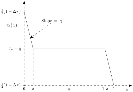
Figure 2: The piecewise linear background profile $\tau_{\delta}(z)$, with $\tau^{\prime}=-\gamma$ in the boundary layer, and $\tau^{\prime}=0$ in the bulk.

Here the single parameter $\delta\leq 1/2$ may be interpreted as modelling the thickness of the thermal boundary layer. The intuition behind this definition is that in order for $\tau(z)$ to be admissible, the indefinite term $\int 2\tau^{\prime}w\theta$ in $\mathcal{Q}^{\prime}_{\tau,R_{\mathrm{e}}}[\mathbf{v},\theta]$ (see (2.45), (2.49)) should be controlled by the other, positive terms. With this choice of background, $2\tau^{\prime}w\theta$ vanishes in the bulk of the domain, and is nonzero only near the fluid boundaries, where $w$ is small. Furthermore, since $\tau^{\prime}$ is piecewise constant, explicit analytical bounds are readily attainable, giving (non-optimal) rigorous bounds on the Nusselt number.

From the definition (4.1), we immediately compute $\tau(0)=\tau_{a}+\gamma\delta$, $\tau(1)=\tau_{a}-\gamma\delta$, and so

$$\Delta\tau=\tau(0)-\tau(1)=2\delta\gamma,\qquad\int_{0}^{1}\tau^{\prime 2}\,dz=2\delta\gamma^{2}=\gamma\Delta\tau,$$ (4.2)

where it remains to choose the average $\tau_{a}=\tfrac{1}{2}(\tau(0)+\tau(1))$ and boundary slope $\gamma=-\tau^{\prime}(0)=-\tau^{\prime}(1)$ of the background as functions of $\delta$. For the mixed (Robin) thermal BCs introduced in Section 3, substituting $\Delta\tau=2\delta\gamma$ into the relation $\Delta\tau+2\eta\gamma=1+2\eta$ (3.8) we obtain the value of $\gamma$ (for given $\delta$ and $\eta$), as well as the corresponding $\Delta\tau$, for which the piecewise linear profile (4.1) satisfies the BCs:

$$\gamma=\frac{1+2\eta}{2(\delta+\eta)},\qquad\Delta\tau=2\delta\gamma=\frac{\delta(1+2\eta)}{\delta+\eta},$$ (4.3)

which implies the related identity $1-\Delta\tau=2\eta(\gamma-1)$; observe that since $\delta\leq 1/2$, we have $1\leq\gamma\leq 1/2\delta$ and $\Delta\tau\leq 1$. Using this $\gamma$ in the BC (3.4) $\tau(0)=1+\eta+\eta\tau^{\prime}(0)$ for $\eta<\infty$, we find that $\tau_{a}=1/2$ (so that we may write $\tau(0)=\tfrac{1}{2}(1+\Delta\tau)$, $\tau(1)=\tfrac{1}{2}(1-\Delta\tau)$), completing the specification of the background $\tau_{\delta}(z)$.

Substituting formulas (4.2)–(4.3) into (3.15)–(3.16) and simplifying, we now find that the conservative bounds on $\beta$ and $\Delta T$ for fixed Biot number convection with a piecewise linear (pwl) background profile $\tau_{\delta}$ take the concise forms

$$\beta\leq\mathcal{B}_{\mathrm{pwl},\eta}(\delta,b)\equiv\mathcal{B}_{\eta}[\tau_{\delta};b] =1+b\,\frac{1}{2}\,\frac{1-2\delta}{\delta+\eta}=1+b(\gamma-1),$$ (4.4)

$$\Delta T\geq\mathcal{D}_{\mathrm{pwl},\eta}(\delta,b)\equiv\mathcal{D}_{\eta}[\tau_{\delta};b] =1-b\,\eta\,\frac{1-2\delta}{\delta+\eta}=1+b(\Delta\tau-1),$$ (4.5)

and the corresponding upper bound on the Nusselt number is $\mathit{Nu}\leq\mathcal{N}_{\mathrm{pwl},\eta}(\delta,b)\equiv\mathcal{N}_{\eta}[\tau_{\delta};b]=\mathcal{B}_{\mathrm{pwl},\eta}(\delta,b)/\mathcal{D}_{\mathrm{pwl},\eta}(\delta,b)$. Since $b>0$, these bounds satisfy $\mathcal{B}_{\mathrm{pwl},\eta}(\delta,b)\geq 1$, $\mathcal{D}_{\mathrm{pwl},\eta}(\delta,b)\leq 1$, and hence $\mathcal{N}_{\mathrm{pwl},\eta}(\delta,b)\geq 1$, as one might expect. Observe that the bounds $\mathcal{B}_{\mathrm{pwl},\eta}(\delta,b)$ and $\mathcal{D}_{\mathrm{pwl},\eta}(\delta,b)$ do not depend explicitly on the control parameter $R$, but rather indirectly through the admissibility condition on $\delta$.

In the special case of fixed temperature BCs, for which $\Delta T=\Delta\tau=1$, we have $\gamma=1/2\delta=\int_{0}^{1}\tau^{\prime 2}\,dz$, and the bound on $\beta$, and hence on the Nusselt number, becomes

$$\mathit{Nu}=\beta\leq\mathcal{B}_{\mathrm{pwl},0}(\delta,b)=1+b\left(\frac{1}{2\delta}-1\right).$$ (4.6)

At the opposite extreme, the fixed flux BCs impose $\beta=\gamma=1$, so that we must choose $\Delta\tau=2\delta=\int_{0}^{1}\tau^{\prime 2}\,dz$; then the lower bound on $\Delta T$ (corresponding to an upper bound on $\mathit{Nu}$) is

$$\mathit{Nu}^{-1}=\Delta T\geq\mathcal{D}_{\mathrm{pwl},\infty}(\delta,b)=1+b(2\delta-1).$$ (4.7)

Again, in this formulation the fixed temperature and fixed flux cases are the $\eta\to 0$ and $\eta\to\infty$ limits of the bounds for general Biot number. We note, however, that the thermal BCs of the form (3.4) do not specify the value of $\tau_{a}$ in the fixed flux case $\eta=\infty$ (the governing equations depend only on temperature gradients, not on their absolute values); here we choose $\tau_{a}=1/2$ for convenience, but use a different choice in the boundedness proof of Appendix A.

4.2 Cauchy-Schwarz estimates on the quadratic form

Recall the admissibility criterion for the background field $\tau_{\delta}(z)$: $\mathcal{Q}^{\prime}_{\tau_{\delta},R_{\mathrm{e}}}[\mathbf{v},\theta]\geq 0$ for all allowed $\mathbf{v}$ and $\theta$, or in Fourier space (by (2.55)–(2.58)) $\mathcal{Q}^{\prime}_{\mathbf{k}}=\mathcal{Q}^{\prime}_{\mathbf{k};\tau_{\delta},R_{\mathrm{e}}}[\hat{w}_{\mathbf{k}},\hat{\theta}_{\mathbf{k}}]\geq 0$ for all $\mathbf{k}$. For piecewise linear background fields $\tau_{\delta}(z)$ of the form (4.1), this criterion reduces to a requirement that $\delta$ is sufficiently small, for given $R_{\mathrm{e}}=bR/(b-1)$. Elementary Cauchy-Schwarz and Young inequalities applied to the Fourier space quadratic form $\mathcal{Q}^{\prime}_{\mathbf{k}}$ allow us to derive explicit sufficient conditions on $\delta$ so that $\mathcal{Q}^{\prime}_{\mathbf{k}}\geq 0$ for all $\mathbf{k}$, and hence to estimate upper bounds on $\mathit{Nu}$.

We recall first that the boundary terms in $\mathcal{Q}^{\prime}_{\tau_{\delta},R_{\mathrm{e}}}[\mathbf{v},\theta]$ for $\eta\in(0,\infty)$ are nonnegative for Robin BCs (and vanish if $\eta=0$ or $\eta=\infty$), so that it is enough to verify the admissibility criterion for $\mathcal{Q}_{\tau_{\delta},R_{\mathrm{e}}}[\mathbf{v},\theta]$ (see the discussion below (3.10)). Equivalently in Fourier space, using (3.12) to evaluate the boundary term in (2.57) for $\eta\in(0,\infty)$, we have

$$\mathcal{Q}^{\prime}_{\mathbf{k}}=\mathcal{Q}_{\mathbf{k}}+\eta\left(|\mathrm{D}\hat{\theta}_{\mathbf{k}}(0)|^{2}+|\mathrm{D}\hat{\theta}_{\mathbf{k}}(1)|^{2}\right)\geq\mathcal{Q}_{\mathbf{k}},$$ (4.8)

so that it suffices to obtain conditions on $\delta$ to ensure $\mathcal{Q}_{\mathbf{k}}\geq 0$ for all $\mathbf{k}$. To do so, we need to control the only indefinite term in $\mathcal{Q}_{\mathbf{k}}$, $\int_{0}^{1}2\tau_{\delta}^{\prime}\text{Re}[\hat{w}_{\mathbf{k}}{\hat{\theta}_{\mathbf{k}}}^{*}]$, by the other terms. For completeness we review the necessary estimates from Otero et al. (2002): Since $\hat{w}_{\mathbf{k}}$ and $\mathrm{D}\hat{w}_{\mathbf{k}}$ (and hence also $\hat{w}_{\mathbf{k}}\,{\hat{\theta}_{\mathbf{k}}}^{*}$) vanish at both boundaries, we have

$$|\hat{w}_{\mathbf{k}}(z)\,{\hat{\theta}_{\mathbf{k}}}^{*}(z)|=\left|\int_{0}^{z}\mathrm{D}\left(\hat{w}_{\mathbf{k}}{\hat{\theta}_{\mathbf{k}}}^{*}\right)\,d\zeta\right|\leq\int_{0}^{z}|\hat{w}_{\mathbf{k}}\mathrm{D}{\hat{\theta}_{\mathbf{k}}}^{*}|\,d\zeta+\int_{0}^{z}|{\hat{\theta}_{\mathbf{k}}}^{*}\mathrm{D}\hat{w}_{\mathbf{k}}|\,d\zeta,$$ (4.9)

where for $0\leq z\leq\tfrac{1}{2}$, by the Fundamental Theorem of Calculus and the Cauchy-Schwarz inequality we find that

$$\left|\hat{w}_{\mathbf{k}}(z)\right|=\left|\int_{0}^{z}\mathrm{D}\hat{w}_{\mathbf{k}}\,d\zeta\right| \leq\sqrt{z}\left(\int_{0}^{z}\left|\mathrm{D}\hat{w}_{\mathbf{k}}(\zeta)\right|^{2}\,d\zeta\right)^{1/2}\leq\sqrt{z}\|\mathrm{D}\hat{w}_{\mathbf{k}}\|_{[0,\tfrac{1}{2}]},$$ (4.10)

$$\left|\mathrm{D}\hat{w}_{\mathbf{k}}(z)\right|=\left|\int_{0}^{z}\mathrm{D}^{2}\hat{w}_{\mathbf{k}}\,d\zeta\right| \leq\sqrt{z}\left(\int_{0}^{z}\left|\mathrm{D}^{2}\hat{w}_{\mathbf{k}}(\zeta)\right|^{2}\,d\zeta\right)^{1/2}\leq\sqrt{z}\|\mathrm{D}^{2}\hat{w}_{\mathbf{k}}\|_{[0,\tfrac{1}{2}]}.$$ (4.11)

Substituting these estimates into (4.9) and again applying the Cauchy-Schwarz inequality, for $0\leq z\leq\tfrac{1}{2}$ we obtain

$$|\hat{w}_{\mathbf{k}}(z)\,{\hat{\theta}_{\mathbf{k}}}^{*}(z)| \leq\left(\int_{0}^{z}\zeta\,d\zeta\right)^{1/2}\left[\|\mathrm{D}\hat{w}_{\mathbf{k}}\|_{[0,\tfrac{1}{2}]}\left(\int_{0}^{z}|\mathrm{D}\hat{\theta}_{\mathbf{k}}|^{2}\,d\zeta\right)^{1/2}\right.$$

$$\qquad\qquad\qquad\quad\ \left.+\|\mathrm{D}^{2}\hat{w}_{\mathbf{k}}\|_{[0,\tfrac{1}{2}]}\left(\int_{0}^{z}|\hat{\theta}_{\mathbf{k}}|^{2}\,d\zeta\right)^{1/2}\right]$$

$$\leq\frac{z}{2\sqrt{2}}\left[a_{1}\|\mathrm{D}\hat{w}_{\mathbf{k}}\|_{[0,\tfrac{1}{2}]}^{2}+\frac{1}{a_{1}}\|\mathrm{D}\hat{\theta}_{\mathbf{k}}\|_{[0,\tfrac{1}{2}]}^{2}+\frac{a_{2}}{k^{2}}\|\mathrm{D}^{2}\hat{w}_{\mathbf{k}}\|_{[0,\tfrac{1}{2}]}^{2}+\frac{k^{2}}{a_{2}}\|\hat{\theta}_{\mathbf{k}}\|_{[0,\tfrac{1}{2}]}^{2}\right],$$ (4.12)

where we have also applied Young’s inequality $pq\leq\tfrac{1}{2}(a_{j}p^{2}+q^{2}/a_{j})$ for any $a_{j}>0$. Proceeding similarly, we obtain an analogous estimate for $\tfrac{1}{2}\leq z\leq 1$. For the piecewise linear background $\tau_{\delta}(z)$, for which $\tau^{\prime}=-\gamma<0$ for $0\leq z\leq\delta$ and $1-\delta\leq 1$, and $\tau^{\prime}=0$ otherwise, applying these estimates we have

$$\left|\int_{0}^{1}\tau_{\delta}^{\prime}\,\hat{w}_{\mathbf{k}}{\hat{\theta}_{\mathbf{k}}}^{*}\,dz\right| \leq\gamma\left(\int_{0}^{\delta}|\hat{w}_{\mathbf{k}}{\hat{\theta}_{\mathbf{k}}}^{*}|\,dz+\int_{1-\delta}^{1}|\hat{w}_{\mathbf{k}}{\hat{\theta}_{\mathbf{k}}}^{*}|\,dz\right)$$

$$\leq\frac{\gamma\delta^{2}}{4\sqrt{2}}\left[a_{1}\|\mathrm{D}\hat{w}_{\mathbf{k}}\|_{[0,1]}^{2}+\frac{1}{a_{1}}\|\mathrm{D}\hat{\theta}_{\mathbf{k}}\|_{[0,1]}^{2}+\frac{a_{2}}{k^{2}}\|\mathrm{D}^{2}\hat{w}_{\mathbf{k}}\|_{[0,1]}^{2}+\frac{k^{2}}{a_{2}}\|\hat{\theta}_{\mathbf{k}}\|_{[0,1]}^{2}\right],$$

and thus

$$\int_{0}^{1}2\tau_{\delta}^{\prime}\text{Re}[\hat{w}_{\mathbf{k}}{\hat{\theta}_{\mathbf{k}}}^{*}]\,dz =\int_{0}^{1}\tau_{\delta}^{\prime}\left(\hat{w}_{\mathbf{k}}{\hat{\theta}_{\mathbf{k}}}^{*}+{\hat{w}_{\mathbf{k}}}^{*}\hat{\theta}_{\mathbf{k}}\right)\,dz$$

$$\geq-\frac{\gamma\delta^{2}}{2\sqrt{2}}\left[a_{1}\|\mathrm{D}\hat{w}_{\mathbf{k}}\|^{2}+\frac{1}{a_{1}}\|\mathrm{D}\hat{\theta}_{\mathbf{k}}\|^{2}+\frac{a_{2}}{k^{2}}\|\mathrm{D}^{2}\hat{w}_{\mathbf{k}}\|^{2}+\frac{k^{2}}{a_{2}}\|\hat{\theta}_{\mathbf{k}}\|^{2}\right],$$ (4.13)

where norms are taken over the entire interval $[0,1]$ unless otherwise indicated. Substituting this estimate on the indefinite term into $\mathcal{Q}_{\mathbf{k}}$ given by (2.56), we find

$$\mathcal{Q}_{\mathbf{k}} \geq\left(\frac{2}{R_{\mathrm{e}}}-\frac{\gamma\delta^{2}\,a_{1}}{2\sqrt{2}}\right)\|\mathrm{D}\hat{w}_{\mathbf{k}}\|^{2}+\left(\frac{1}{R_{\mathrm{e}}}-\frac{\gamma\delta^{2}\,a_{2}}{2\sqrt{2}}\right)\frac{1}{k^{2}}\|\mathrm{D}^{2}\hat{w}_{\mathbf{k}}\|^{2}+\frac{1}{R_{\mathrm{e}}}k^{2}\|\hat{w}_{\mathbf{k}}\|^{2}$$

$$\qquad+\left(1-\frac{\gamma\delta^{2}}{2\sqrt{2}\,a_{2}}\right)k^{2}\|\hat{\theta}_{\mathbf{k}}\|^{2}+\left(1-\frac{\gamma\delta^{2}}{2\sqrt{2}\,a_{1}}\right)\|\mathrm{D}\hat{\theta}_{\mathbf{k}}\|^{2}.$$

In the absence of any additional a priori information, for instance on the decay rate of the Fourier coefficients (compare Constantin & Doering (1996); Kerswell (2001)), our remaining estimates are necessarily $k$-independent; we ensure the positivity of $\mathcal{Q}_{\mathbf{k}}$ by requiring all coefficients to be nonnegative. We choose $a_{1}=a_{2}=\gamma\delta^{2}/2\sqrt{2}$; then, using (4.8) and dropping manifestly nonnegative terms,

$$\mathcal{Q}^{\prime}_{\mathbf{k}}\geq\mathcal{Q}_{\mathbf{k}}\geq\left(\frac{2}{R_{\mathrm{e}}}-\frac{\gamma^{2}\delta^{4}}{8}\right)\|\mathrm{D}\hat{w}_{\mathbf{k}}\|^{2}+\left(\frac{1}{R_{\mathrm{e}}}-\frac{\gamma^{2}\delta^{4}}{8}\right)\frac{1}{k^{2}}\|\mathrm{D}^{2}\hat{w}_{\mathbf{k}}\|^{2}.$$ (4.14)

We can thus guarantee that $\mathcal{Q}_{\mathbf{k}}\geq 0$ (and hence $\mathcal{Q}^{\prime}_{\mathbf{k}}\geq 0$) if we choose $\gamma^{2}\delta^{4}/8\leq 1/R_{\mathrm{e}}$. For given thermal BCs, $\gamma=\gamma(\delta)$ is specified as a function of $\delta$; so this is a constraint on $\delta$ to have $\mathcal{Q}_{\mathbf{k}}\geq 0$, that is, for $\tau_{\delta}(z)$ to be an admissible background. Defining $\delta_{c}$ by

$$\gamma(\delta_{c})^{2}\delta_{c}^{4}=\frac{8}{R_{\mathrm{e}}}=8\frac{b-1}{bR},$$ (4.15)

we obtain the best bound in this approach by choosing $\delta=\delta_{c}$; the piecewise linear profile $\tau_{\delta}$ is admissible for any $\delta\leq\delta_{c}$.

We observe that the estimates (4.9)–(4.14), and hence the sufficient condition (4.15) on $\delta$, are independent of the choice of boundary conditions on $\hat{\theta}_{\mathbf{k}}$ at $z=0,1$ (apart from symmetry). However, the thermal BCs enter the admissibility condition on $\tau_{\delta}$ through the value (4.3) of $\gamma=\gamma(\delta)$ as a function of $\eta$.

5 Explicit asymptotic bounds for general thermal boundary conditions

Using the piecewise linear background profile $\tau_{\delta}(z)$ and estimates introduced in Section 4, we may now derive explicit analytical bounds on the growth of the Nusselt number $\mathit{Nu}$ with the control parameter $R$, and hence with the Rayleigh number $\mathit{Ra}$, for thermal boundary conditions with fixed Biot number $0\leq\eta\leq\infty$. We begin as usual by recalling the results for Dirichlet ($\eta=0$) and Neumann ($\eta=\infty$) BCs, as in the general case it then becomes apparent that the fixed temperature case is a singular limit, while for any $\eta>0$, the $R\to\infty$ asymptotic scaling is as in the fixed flux case. In this Section we summarize the main asymptotic bounds; more details including discussion of different scaling regimes for $0<\eta<\infty$ will be given elsewhere (Wittenberg & Gao (2008); see also Gao (2006)), while rigorous, though somewhat weaker, bounds are proved in Appendix C.

5.1 Fixed temperature boundary conditions

In the case of Dirichlet BCs, we have $\Delta T=\Delta\tau=1$, $R=\mathit{Ra}$, and (4.3) implies $\gamma=1/2\delta$. Thus the sufficient condition (4.15) on $\delta$ simplifies to $\delta\leq\delta_{c}$ where

$$\delta_{c}^{2}=\frac{32}{R_{\mathrm{e}}}=32\frac{b-1}{bR}.$$ (5.1)

One can show that the optimal choice of $b$ in this formulation is $b_{0}=3/2$ (see Wittenberg & Gao (2008)), for which $R_{\mathrm{e}}=3R$, and hence $\delta\leq\delta_{c}=4\sqrt{2/3}\,R^{-1/2}$ is sufficient to obtain a rigorous bound. Since for this $b=b_{0}$, (4.6) becomes

$$\mathit{Nu}=\beta\leq\mathcal{B}_{\mathrm{pwl},0}(\delta,b_{0})=1-b_{0}+\frac{b_{0}}{2\delta}=-\frac{1}{2}+\frac{3}{4\delta},$$ (5.2)

for any $\delta\leq\delta_{c}$, the best rigorous analytical bound on the Nusselt number using this approach is

$$\mathit{Nu}\leq\tilde{\mathcal{N}}_{\text{pwl}}(R)=\mathcal{B}_{\mathrm{pwl},0}(\delta_{c},b_{0})=-\frac{1}{2}+\frac{3}{4\delta_{c}}=-\frac{1}{2}+\frac{3}{16}\sqrt{\frac{3}{2}}R^{1/2}=-\frac{1}{2}+\frac{3\sqrt{6}}{32}\mathit{Ra}^{1/2},$$ (5.3)

where we used the fact that for fixed temperature BCs, the control parameter $R$ is the usual Rayleigh number $\mathit{Ra}$.

5.2 Fixed flux boundary conditions

In the opposite extreme, for Neumann BCs, we have $\beta=\gamma=1$, and we bound $\Delta T$ from below using (4.7). Since $b>1$, in order for the lower bound $\mathcal{D}_{\mathrm{pwl},\infty}(\delta,b)=1-b+2\delta\,b$ on $\Delta T$ to remain positive as $R\to\infty$ and hence $\delta\to 0$, we need $b-1={\mathcal{O}}(\delta)$. Thus following Otero et al. (2002) we choose $b=1+c\,\delta$ and let $c$ take its optimal value $c_{\infty}=1/2$, so that (4.7) becomes

$$\mathit{Nu}^{-1}=\Delta T\geq\mathcal{D}_{\mathrm{pwl},\infty}(\delta,1+c_{\infty}\delta)=1+(1+\delta/2)(2\delta-1)=\frac{3}{2}\delta+\delta^{2}\sim\frac{3}{2}\delta.$$ (5.4)

The condition on $\delta$ is as usual $\delta\leq\delta_{c}$, where with $\gamma=1$ and $b=1+\delta/2$, the equation (4.15) satisfied by $\delta_{c}$ takes the form

$$\delta^{4}=\frac{8}{R_{\mathrm{e}}}=4\frac{\delta}{1+\delta/2}R^{-1}\sim 4\frac{\delta}{R}$$ (5.5)

for large $R$, for which $\delta\to 0$; and hence $\delta_{c}\sim 4^{1/3}R^{-1/3}$. Thus we have (using (2.15))

$$\mathit{Nu}^{-1}=\Delta T \geq\mathcal{D}_{\mathrm{pwl},\infty}(\delta_{c},1+\delta_{c}/2)\sim\frac{3}{2}\delta_{c}\sim\frac{3}{2^{1/3}}R^{-1/3},$$

$$\mathit{Ra}=R\Delta T \geq R\,\mathcal{D}_{\mathrm{pwl},\infty}(\delta_{c},1+\delta_{c}/2)\sim\frac{3}{2^{1/3}}R^{2/3},$$

and so

$$\mathit{Nu}\leq\tilde{\mathcal{N}}_{\text{pwl}}(R)\lesssim\frac{2^{1/3}}{3}R^{1/3}\lesssim\sqrt{\frac{2}{27}}\mathit{Ra}^{1/2},$$ (5.6)

as in Otero et al. (2002). Note the scaling $\mathit{Nu}\leq C_{1}R^{1/3}$ in terms of the control parameter $R$, which translates to the usual scaling $\mathit{Nu}\leq C_{2}\mathit{Ra}^{1/2}$.

5.3 Mixed thermal boundary conditions with fixed Biot number

For general mixed (Robin) thermal BCs with fixed Biot number, we need to estimate both $\Delta T$ and $\beta$, using (4.4) and (4.5), where $\gamma$ and $\Delta\tau$ are given in terms of $\eta$ and $\delta$ by (4.3). The sufficient condition $\delta\leq\delta_{c}$ for $\tau_{\delta}$ to be admissible, derived via the Cauchy-Schwarz estimates of Section 4.2, is that $\delta_{c}$ satisfies (4.15), which (substituting for $\gamma$ from (4.3)) here takes the form

$$\gamma^{2}\delta^{4}=\frac{(1+2\eta)^{2}}{4(\delta+\eta)^{2}}\delta^{4}=\frac{8}{R_{\mathrm{e}}}=8\frac{b-1}{b}R^{-1}.$$ (5.7)

We shall see that in this general case with $0<\eta<\infty$, depending on the relative sizes of $\delta$ and $\eta$, the scaling of the bounds behaves either as in the fixed temperature limit (for $\delta\geq\eta$) or the fixed flux limit (for $\delta\leq\eta$); but that for any $\eta>0$, the asymptotic scaling as $R\to\infty$ is as for fixed flux boundary conditions:

The fixed temperature problem $\eta=0$ as a singular limit:

Recall that for Dirichlet thermal boundary conditions $\eta=0$, we have $\Delta T=\Delta\tau=1$, so that we obtain an upper bound on $\mathit{Nu}$ for any $b>0$ (there is no concern that the lower bound $\mathcal{D}_{\mathrm{pwl},0}$ on $\Delta T$ may become negative), and we can choose $b-1={\mathcal{O}}(1)$ for all $\delta$. In this case $\eta=0$, though, $\gamma=1/2\delta$ is not bounded above as $R\to\infty$ ($\delta\to 0$), and hence neither is $\beta$; the growth in the (upper bound for) the Nusselt number in the fixed temperature case with increasing control parameter $R=\mathit{Ra}$ is due to that of the (non-dimensional) boundary heat flux.

The situation is quite different for any nonzero Biot number $\eta$: since $0<\delta\leq 1/2$, we have $0\leq(1-2\delta)/2(\delta+\eta)=\gamma-1<1/2\eta$, so that now $\gamma$ is bounded above as $\delta\to 0$ for $\eta>0$. On the other hand, $\Delta\tau=2\delta\gamma$ is not bounded away from zero, so that since $b>1$, to get a positive value for the lower bound $\mathcal{D}_{\mathrm{pwl},\eta}=1-b+b\Delta\tau$ for sufficiently large $R$ (small $\delta$), we need $b-1={\mathcal{O}}(\delta)$ for each fixed $\eta>0$. Furthermore, we have $\Delta T\to 0$ as $R\to\infty$, so that (for sufficiently large $R$) the growth in the Nusselt number bound is due to the decrease in $\Delta T$, the (non-dimensional) averaged temperature drop across the fluid, rather than due to the growth in $\beta$. That is, for any $\eta>0$ the (asymptotic) behaviour and scaling is as in the fixed flux case; the fixed temperature problem is a singular limit. (A similar observation was made in the context of horizontal convection by Siggers et al. (2004).)

Scaling regimes:

More precisely, the nature of the $\mathit{Nu}$-$R$ scaling depends on whether $\delta\geq\eta$ or $\delta\leq\eta$, and hence on the value of $\eta$:

For sufficiently large Biot number (largely insulating boundary) $\eta\geq 1/2$, we always have $\delta\leq\eta$. Since for such $\eta$, $\gamma$ is approximately constant ($1\leq\gamma<1+1/2\eta\leq 2$; compare $\gamma=1$ for $\eta=\infty$), we see from (5.7) that a sufficient admissibility condition for $\tau_{\delta}$ is $\delta\leq\delta_{c}={\mathcal{O}}(R_{\mathrm{e}}^{-1/4})$, as in the fixed flux case. We choose $b=1+c\delta\leq 3/2$ for some $c\leq 1$, so $\beta\leq 1+b(\gamma-1)\leq 5/2$ for all $\delta\leq 1/2$, and there is no transition in scaling regimes; as in the fixed flux case, for all sufficiently large $\eta$ the growth in $\mathit{Nu}$ is due to the decrease in $\Delta T$.

For relatively small Biot number (largely conducting boundary) $\eta<1/2$, on the other hand, it is possible to have $\delta\geq\eta$ for low enough thermal driving, and thus distinct regimes exist. In particular, consider the case of small Biot number ($\eta\ll 1$, near the fixed temperature limit), where we can identify two distinct scaling behaviours:

• “Fixed temperature scaling”: For sufficiently small $R$, we have $\delta\gg\eta$, so that $\gamma\sim 1/2\delta$ and $\Delta\tau\sim 1$, and the sufficiency condition (5.7) is $\delta\leq\delta_{c}={\mathcal{O}}(R_{\mathrm{e}}^{-1/2})$. Since $\Delta\tau$ is bounded below away from zero, so is the lower bound $\mathcal{D}_{\mathrm{pwl},\eta}(\delta,b)=1+b(\Delta\tau-1)\geq 1-b/2$ on $\Delta T$ for any fixed $b<2$. Thus we may obtain a bound on $\mathit{Nu}$ in this regime by choosing any $b\in(1,2)$, and by comparison with the fixed temperature problem, it is sufficient to choose $b-1={\mathcal{O}}(1)$, in which case we have $\delta_{c}={\mathcal{O}}([(b-1)/bR]^{1/2})={\mathcal{O}}(R^{-1/2})$. While $\Delta T={\mathcal{O}}(1)$ (so that $\mathit{Ra}={\mathcal{O}}(R)$), we have that $\beta\leq\mathcal{B}_{\mathrm{pwl},\eta}(\delta,b)=1+b(\gamma-1)={\mathcal{O}}(b/\delta)$ grows as $\delta^{-1}$. Thus clearly when $\eta\ll 1$, for sufficiently small but increasing $R$, the scaling properties are as in the fixed temperature case, and the growth in $\mathit{Nu}=\beta/\Delta T$ is driven by that of $\beta$.

  As the driving $R$ increases, $\delta$ decreases, and eventually becomes less than the Biot number $\eta$; based on the fixed temperature scaling $\delta={\mathcal{O}}(R^{-1/2})={\mathcal{O}}(\mathit{Ra}^{-1/2})$ the transition at $\delta=\eta$ occurs when $\eta={\mathcal{O}}(\mathit{Ra}^{-1/2})$, or $\mathit{Ra}={\mathcal{O}}(\eta^{-2})$.

• “Fixed flux scaling”: Once the “boundary layer thickness” $\delta$ has decreased below $\eta>0$ for increasing $R$, we enter another regime (which does not exist in the fixed temperature case $\eta=0$), in which for fixed $\eta$ the growth in $\gamma$ saturates, while $\Delta\tau={\mathcal{O}}(\delta)$ decreases. Asymptotically for $\delta\ll\eta$, we have $\gamma\sim(1+2\eta)/2\eta=\gamma_{\text{max}}(\eta)$, while $\Delta\tau\sim\delta(1+2\eta)/\eta$, and for each fixed $\eta>0$ the behaviour is now as if we had Neumann thermal BCs.

  More generally, for $0<\eta\leq 1/2$ and decreasing $\delta\leq\eta$, we have $\gamma={\mathcal{O}}(\eta^{-1})$ and $\Delta\tau={\mathcal{O}}(\delta/\eta)$. In order for the lower bound $\mathcal{D}_{\mathrm{pwl},\eta}=1-b+b\Delta\tau$ on $\Delta T$ to remain positive as $\delta\to 0$, we must choose $b=1+{\mathcal{O}}(\delta/\eta)$, so that $\beta\leq\mathcal{B}_{\mathrm{pwl},\eta}=1+b(\gamma-1)={\mathcal{O}}(\eta^{-1})$ saturates, while $\Delta T\geq{\mathcal{O}}(\delta/\eta)$; hence the growth in $\mathit{Nu}$ is now due to the decay in $\Delta T$, as in the fixed flux case. In this regime the scaling behaviours are $\mathit{Ra}\geq{\mathcal{O}}(\delta R/\eta)$, $R_{\mathrm{e}}={\mathcal{O}}(\eta R/\delta)$ and $\delta={\mathcal{O}}(\gamma^{-1/2}R_{\mathrm{e}}^{-1/4})={\mathcal{O}}(\eta^{1/3}R^{-1/3})={\mathcal{O}}(\mathit{Ra}^{-1/2})$; more precise asymptotic statements are given below, with weaker, but rigorous results in Appendix C.

Asymptotic scaling of bounds for $0<\eta<\infty$:

Having outlined the behaviour in the different regimes, we here derive the scaling of the bound on the Nusselt number in the limit of large driving, $R\to\infty$, so that $\delta\ll 1$ and $\delta\ll\eta$, deferring a more detailed discussion of scaling behaviour in the different regimes using this Cauchy-Schwarz analysis, and a comparison with numerical solutions for piecewise linear backgrounds, to Wittenberg & Gao (2008).

In the light of the above discussion, for $\delta\ll\eta$ we must choose $b=1+c\,\delta$, where the optimal value of $c$ turns out to be

$$c_{\eta}=\frac{1+2\eta}{4\eta}.$$ (5.8)

Using this optimal choice of $b$, the lower bound (4.5) on $\Delta T$ becomes

$$\Delta T\geq\mathcal{D}_{\mathrm{pwl},\eta}(\delta,1+c_{\eta}\delta) =-c_{\eta}\delta+(1+c_{\eta}\delta)\frac{\delta(1+2\eta)}{\delta+\eta}$$

$$=\frac{\delta(1+2\eta)}{\delta+\eta}\frac{3+2\delta}{4}\sim\frac{3}{4}\frac{\delta(1+2\eta)}{\eta},$$ (5.9)

while similarly, the upper bound (4.4) is

$$\beta\leq\mathcal{B}_{\mathrm{pwl},\eta}(\delta,1+c_{\eta}\delta) =-c_{\eta}\delta+(1+c_{\eta}\delta)\frac{1+2\eta}{2(\delta+\eta)}$$

$$=\frac{1+2\eta}{2(\delta+\eta)}\left[1+\frac{\delta}{4\eta}(1-2\delta)\right]\sim\frac{1+2\eta}{2\eta},$$ (5.10)

so that an upper bound on the Nusselt number for admissible $\delta\ll\eta$ is

$$\mathit{Nu}=\frac{\beta}{\Delta T}\leq\mathcal{N}_{\mathrm{pwl},\eta}(\delta,1+c_{\eta}\delta)=\frac{1}{2\delta}\frac{4+\delta(1-2\delta)/\eta}{3+2\delta}\sim\frac{2}{3\delta};$$ (5.11)

compare (5.2) and (5.4).

Observe that the width $\delta_{\text{BL}}$ of the thermal boundary layer is often related to the Nusselt number via $\delta_{\text{BL}}=(2\mathit{Nu})^{-1}$ (Niemela & Sreenivasan (2006b)); our high-$R$ result for the piecewise linear background, $\delta\sim(3\mathit{Nu}/2)^{-1}$ for $\eta>0$ (or $\delta\sim(4\mathit{Nu}/3)^{-1}$ for $\eta=0$), may be interpreted as a systematic statement of such a boundary layer model.

Returning to the computation of asymptotic bounds, we note from (5.8) that for $\eta\geq 1/2$, $c_{\eta}=1/2+1/4\eta\leq 1$, while for $\eta\leq 1/2$, $c_{\eta}\delta=(1+2\eta)\delta/4\eta\leq\delta/2\eta$, so that whenever $\delta\ll\min(\eta,1)$ we have $c_{\eta}\delta\ll 1$; consequently $b=1+c_{\eta}\delta\sim 1$ and $R_{\mathrm{e}}=b\,R/(b-1)\sim R/c_{\eta}\delta$. In this case the condition (5.7) is thus

$$\delta^{4}=32\frac{(\delta+\eta)^{2}}{(1+2\eta)^{2}}R_{\mathrm{e}}^{-1}\sim 32\frac{\eta^{2}}{(1+2\eta)^{2}}\frac{1+2\eta}{4\eta}\delta R^{-1}=8\frac{\eta}{1+2\eta}\delta R^{-1},$$ (5.12)

or $\delta_{c}\sim 2\eta^{1/3}(1+2\eta)^{-1/3}R^{-1/3}$. Substituting into the above bounds, we have

$$\mathit{Nu}\leq\mathcal{N}_{\mathrm{pwl},\eta}(\delta_{c},1+c_{\eta}\delta_{c}) \sim\frac{2}{3\,\delta_{c}}\sim\frac{1}{3}\left(\frac{1+2\eta}{\eta}\right)^{1/3}R^{1/3},$$ (5.13)

$$\mathit{Ra}=R\Delta T\geq R\mathcal{D}_{\mathrm{pwl},\eta}(\delta_{c},1+c_{\eta}\delta_{c}) \sim\frac{3}{4}\frac{1+2\eta}{\eta}\,\delta_{c}\,R\sim\frac{3}{2}\left(\frac{1+2\eta}{\eta}\right)^{2/3}R^{2/3},$$ (5.14)

so that we obtain a bound on the asymptotic scaling as $R\to\infty$ of the Nusselt number with the Rayleigh number whenever $\eta>0$:

$$\mathit{Nu}\lesssim\frac{1}{3}\left(\frac{1+2\eta}{\eta}\right)^{1/3}\sqrt{\frac{2}{3}}\left(\frac{\eta}{1+2\eta}\right)^{1/3}\mathit{Ra}^{1/2}=\sqrt{\frac{2}{27}}\mathit{Ra}^{1/2},$$ (5.15)

independent of the Biot number. Observe in particular, by comparison with (5.6), that the prefactor $\sqrt{2/27}$ is the same as for the fixed flux problem.

6 Conclusions

In formulating the energy identities and bounding problem for the Rayleigh-Bénard model with finite Prandtl number and general thermal BCs at the upper and lower boundaries of the fluid, we have demonstrated that the fixed temperature and fixed flux extremes may indeed be treated as special cases of a more general model, within which one can rigorously prove energy boundedness and bounds on convective heat transport, and obtain asymptotic scaling results; we expect that such an approach may be applicable to other related convection problems.

While the scaling of these analytical bounds on the $\mathit{Nu}$–$\mathit{Ra}$ relationship remains well above that observed experimentally or in direct numerical simulations, some of the qualitative conclusions may be instructive. Of particular interest is that—at least for the piecewise linear backgrounds $\tau_{\delta}(z)$ treated here—while for each fixed $R$ the bounds depend smoothly on $\eta$ for $0\leq\eta\leq\infty$, the asymptotic $R\to\infty$ scaling of the bound for any nonzero Biot number is as for the $\eta=\infty$ fixed flux problem. That is, the limits $\eta\to 0$ and $R\to\infty$ do not commute: fixed temperature conditions in fact form a singular limit.

Furthermore, the bounding calculation indicates the existence of two distinct scaling behaviours for sufficiently small nonzero $\eta$; it would be of interest to observe these in fixed Biot number direct numerical simulations: For small Rayleigh number $\mathit{Ra}$, there is a “fixed temperature scaling regime” in which the usual assumption of Dirichlet thermal BCs is approximately valid, as the growth in the convective heat transport measured by $\mathit{Nu}$ is largely due to the increase in the averaged boundary heat flux $\beta$. As the control parameter $R$, and hence $\mathit{Ra}$, increases, a transition occurs when the “boundary layer width” $\delta$ becomes comparable to $\eta$ (in our calculations this occurs for $\mathit{Ra}={\mathcal{O}}(\eta^{-2})$), beyond which a “fixed flux scaling regime” is entered, in which further increases in $\mathit{Nu}$ are driven by decreases in the averaged temperature drop $\Delta T$. This observation provides mathematical support for the heuristic argument that when the Nusselt number is sufficiently high, the boundaries act effectively as insulators.

In the three-dimensional simulations of Verzicco & Sreenivasan (2008) in cylindrical geometry with perfectly insulating sidewalls and a perfectly conducting upper boundary, replacing the lower fixed temperature BCs with fixed flux conditions was observed to have little effect on the heat transport for a given Rayleigh number for sufficiently small $\mathit{Ra}\lesssim 10^{9}$, and to decrease the transport for $\mathit{Ra}>10^{9}$. In constrast, the two-dimensional, horizontally periodic computations of Johnston & Doering (2008) showed essentially identical heat transport for fixed temperature and fixed flux BCs at both upper and lower plates for $10^{7}\lesssim\mathit{Ra}\lesssim 10^{10}$. In this context we observe that the prefactor in our asymptotic analytical bound $\mathit{Nu}\leq C\,\mathit{Ra}^{1/2}$ increases from $C_{0}=3\sqrt{6}/32\approx 0.230$ to $C_{\eta}=C_{\infty}=\sqrt{2/27}\approx 0.272$ for $\eta>0$; that is, within the framework of our upper bounding calculations with piecewise linear background it appears that the estimates on the heat transport increase when the boundaries are not perfectly conducting. It remains to determine whether this increase is an artifact of the choice of background $\tau(z)$ or of the background flow bounding approach in general. A further consideration is how the presence of finite width conducting plates (see Part 2 of this work) modifies conclusions obtained with the fixed Biot number simplification.

Acknowledgments

I would like to thank Charlie Doering, Jian Gao, Jesse Otero and Jean-Luc Thiffeault for useful discussions concerning this work. This research was partially supported by grants from the Natural Sciences and Engineering Research Council of Canada (NSERC).

Appendix A Boundedness of $\|T\|^{2}$ and $\|\mathbf{u}\|^{2}$

For completeness of the rigorous argument, we show the uniform boundedness of the temperature and velocity fields, which we may state as a theorem:

Theorem 1

The velocity field $\mathbf{u}$ and temperature field $T$ satisfying (2.7)–(2.9) for finite Prandtl number, $0<\mathit{Pr}<\infty$, and for no-slip velocity boundary conditions and thermal boundary conditions of general Biot number $0\leq\eta\leq\infty$, are uniformly bounded in $\mathrm{L}^{2}$.

Remark A.1.

Such boundedness has already been shown for Rayleigh-Bénard convection with fixed temperature BCs by Kerswell (2001), following the underlying approach introduced by Doering & Constantin (1992) (based on an idea of Hopf (1941)) in the context of shear flow. However, in both of these cases the Dirichlet boundary conditions allow ready control of the indefinite term in real space; since for general thermal BCs we are not assured control of $\theta$ at the fluid boundaries, in our proof instead we use incompressibility and Fourier space estimates based on those of Otero et al. (2002).

Proof A.2.

We begin the demonstration of Theorem 1 by reviewing the basic problem formulation and identities: With thermal boundary conditions imposed at the upper and lower limits of the fluid, we consider horizontally periodic temperature and velocity fields $T(\mathbf{x},t)$ and $\mathbf{u}(\mathbf{x},t)$ satisfying (2.7)–(2.9), where $\mathbf{u}$ satisfies incompressibility and no-slip BCs. Choosing a background temperature field $\tau(z)$ which satisfies the given thermal boundary conditions, we define $\mathbf{v}(\mathbf{x},t)$ and $\theta(\mathbf{x},t)$ via the decomposition (2.33), $\mathbf{u}(\mathbf{x},t)=\mathbf{v}(\mathbf{x},t)$, $T(\mathbf{x},t)=\tau(z)+\theta(\mathbf{x},t)$, and thus obtain the evolution equations (2.39)–(2.40) for their $\mathrm{L}^{2}$ norms:

$$\frac{1}{2\mathit{Pr}R}\frac{d}{dt}\left\|\mathbf{v}\right\|^{2} =-\frac{1}{R}\left\|\mbox{\boldmath$\nabla$\unboldmath}\mathbf{v}\right\|^{2}+\int w\theta,$$ (A.1)

$$\frac{1}{2}\frac{d}{dt}\left\|\theta\right\|^{2} =-\left\|\mbox{\boldmath$\nabla$\unboldmath}\theta\right\|^{2}+A\left.\overline{\theta\theta_{z}}\right|_{z=0}^{1}-\int\theta_{z}\tau^{\prime}+A\left.\overline{\theta}\tau^{\prime}\right|_{z=0}^{1}-\int w\theta\tau^{\prime}.$$ (A.2)

We form the linear combination (A.1) + $\mu\cdot$(A.2), where the weight $\mu$ will be chosen later:

$$\frac{1}{2}\frac{d}{dt}\left[\left\|\theta\right\|^{2}+\frac{\mu}{\mathit{Pr}R}\left\|\mathbf{v}\right\|^{2}\right] =-\frac{\mu}{R}\left\|\mbox{\boldmath$\nabla$\unboldmath}\mathbf{v}\right\|^{2}+\mu\int w\theta-\int\tau^{\prime}w\theta-\left\|\mbox{\boldmath$\nabla$\unboldmath}\theta\right\|^{2}$$

$$\qquad\ -\int\tau^{\prime}\theta_{z}+A\left.\overline{\theta\theta_{z}}\right|_{z=0}^{1}+A\left.\overline{\theta}\tau^{\prime}\right|_{z=0}^{1}.$$ (A.3)

We choose, as before, a piecewise linear $\tau(z)$, defined as in (4.1) and figure 2 for $0<\delta\leq 1/2$:

$$\tau(z)=\left\{\begin{array}[]{ll}\tau_{a}-\gamma(z-\delta),&0\leq z\leq\delta,\\ \tau_{a},&\delta<z<1-\delta,\\ \tau_{a}-\gamma(z-1+\delta),&1-\delta\leq z\leq 1;\\ \end{array}\right.$$ (A.4)

As in Section 4.1, we find using the thermal BCs that (4.3) $\gamma=-\tau^{\prime}(0)=-\tau^{\prime}(1)=(1+2\eta)/2(\delta+\eta)$, while for $\eta<\infty$ we also have $\tau_{a}=1/2$; for now we defer the (at present arbitrary) choice of $\tau_{a}$ in the fixed flux case $\eta=\infty$.

A.1 Estimates independent of thermal BCs:

The estimates on the indefinite quadratic terms are performed in Fourier space using the definition (2.54), while other terms are readily controlled in real space; thus we split the dissipative terms as

$$\left\|\mbox{\boldmath$\nabla$\unboldmath}\theta\right\|^{2}=\left(\frac{1}{2}+\frac{1}{2}\right)\int|\mbox{\boldmath$\nabla$\unboldmath}\theta|^{2}=\frac{1}{2}\left\|\mbox{\boldmath$\nabla$\unboldmath}\theta\right\|^{2}+\frac{1}{2}A\sum_{\mathbf{k}}\int_{0}^{1}\left(k^{2}|\hat{\theta}_{\mathbf{k}}|^{2}+|\mathrm{D}\hat{\theta}_{\mathbf{k}}|^{2}\right)\,dz$$ (A.5)

and, using incompressibility,

$$\left\|\mbox{\boldmath$\nabla$\unboldmath}\mathbf{v}\right\|^{2}\geq\frac{1}{2}\left\|\mbox{\boldmath$\nabla$\unboldmath}\mathbf{v}\right\|^{2}+\frac{1}{2}A\sum_{\mathbf{k}}\int_{0}^{1}\left(k^{2}|\hat{w}_{\mathbf{k}}|^{2}+2|\mathrm{D}\hat{w}_{\mathbf{k}}|^{2}+\frac{1}{k^{2}}|\mathrm{D}^{2}\hat{w}_{\mathbf{k}}|^{2}\right)\,dz,$$ (A.6)

with equality for two-dimensional flows.

We bound $\int w\theta$ using estimates of the form (4.12), which imply that for $\mathbf{k}\not=\mathbf{0}$, any $0<\delta\leq 1/2$ and any $p,q>0$,

$$\begin{split}\left(\int_{0}^{\delta}|\hat{w}_{\mathbf{k}}\right)&\\ \leq\frac{\delta^{2}}{4\sqrt{2}}&\left[p\|\mathrm{D}\hat{w}_{\mathbf{k}}\|^{2}+\frac{1}{p}\|\mathrm{D}\hat{\theta}_{\mathbf{k}}\|^{2}+\frac{q}{k^{2}}\|\mathrm{D}^{2}\hat{w}_{\mathbf{k}}\|^{2}+\frac{k^{2}}{q}\|\hat{\theta}_{\mathbf{k}}\|^{2}\right].\end{split}$$ (A.7)

In particular, using (A.7) with $\delta=1/2$, recalling $\hat{w}_{\mathbf{0}}=0$,

$$\frac{1}{A}\int w\theta =\sum_{\mathbf{k}}\int_{0}^{1}\text{Re}[\hat{w}_{\mathbf{k}}$$

$$\leq\frac{1}{16\sqrt{2}}\sum_{\mathbf{k}}\left[a_{1}\|\mathrm{D}\hat{w}_{\mathbf{k}}\|^{2}+\frac{1}{a_{1}}\|\mathrm{D}\hat{\theta}_{\mathbf{k}}\|^{2}+\frac{a_{2}}{k^{2}}\|\mathrm{D}^{2}\hat{w}_{\mathbf{k}}\|^{2}+\frac{k^{2}}{a_{2}}\|\hat{\theta}_{\mathbf{k}}\|^{2}\right].$$ (A.8)

Similarly, using the definition (A.4) of $\tau(z)$, as in (4.13) we have

$$\frac{1}{A}\left|\int\tau^{\prime}w\theta\right| \leq\frac{1}{2}\sum_{\mathbf{k}}\left|\int_{0}^{1}\tau^{\prime}(\hat{w}_{\mathbf{k}}\right|$$

$$\leq\frac{\gamma\delta^{2}}{4\sqrt{2}}\sum_{\mathbf{k}}\left[a_{3}\|\mathrm{D}\hat{w}_{\mathbf{k}}\|^{2}+\frac{1}{a_{3}}\|\mathrm{D}\hat{\theta}_{\mathbf{k}}\|^{2}+\frac{a_{4}}{k^{2}}\|\mathrm{D}^{2}\hat{w}_{\mathbf{k}}\|^{2}+\frac{k^{2}}{a_{4}}\|\hat{\theta}_{\mathbf{k}}\|^{2}\right].$$ (A.9)

The other two terms in (A.3) containing $\tau^{\prime}$ may be estimated directly, since for any $a_{5}>0$, we have (also using $\|\theta_{z}\|\leq\|\mbox{\boldmath$\nabla$\unboldmath}\theta\|$)

$$-\int\tau^{\prime}\theta_{z}+A\left.\tau^{\prime}\overline{\theta}\right|_{z=0}^{1} =\gamma A\left(\int_{0}^{\delta}\overline{\theta}_{z}\,dz+\int_{1-\delta}^{1}\overline{\theta}_{z}\,dz\right)-\gamma A\int_{0}^{1}\overline{\theta}_{z}\,dz$$

$$=-\gamma A\int_{\delta}^{1-\delta}\overline{\theta}_{z}\,dz=-\gamma\int_{\delta}^{1-\delta}\iint_{A}\theta_{z}\,dx\,dy\,dz$$

$$\leq\gamma A^{1/2}\sqrt{1-2\delta}\left(\int_{\delta}^{1-\delta}\iint_{A}\theta_{z}^{2}\,dx\,dy\,dz\right)^{1/2}$$

$$\leq\gamma A^{1/2}\|\theta_{z}\|\leq\frac{1}{2}\left(a_{5}\gamma^{2}A+\frac{1}{a_{5}}\|\mbox{\boldmath$\nabla$\unboldmath}\theta\|^{2}\right).$$ (A.10)

Substituting (A.5)–(A.10) into (A.3), and collecting like terms, we thus obtain

$$\frac{1}{2}\frac{d}{dt}\left[\left\|\theta\right\|^{2}+\frac{\mu}{\mathit{Pr}R}\left\|\mathbf{v}\right\|^{2}\right] \leq\frac{1}{2}a_{5}\gamma^{2}A-\frac{\mu}{2R}\left\|\mbox{\boldmath$\nabla$\unboldmath}\mathbf{v}\right\|^{2}-\frac{1}{2}\left(1-\frac{1}{a_{5}}\right)\left\|\mbox{\boldmath$\nabla$\unboldmath}\theta\right\|^{2}+A\left.\overline{\theta\theta_{z}}\right|_{z=0}^{1}$$

$$\quad-A\sum_{\mathbf{k}}\frac{\mu}{2R}k^{2}\|\hat{w}_{\mathbf{k}}\|^{2}-A\sum_{\mathbf{k}}\left(\frac{\mu}{R}-\frac{a_{1}\mu}{16\sqrt{2}}-\frac{a_{3}\gamma\delta^{2}}{4\sqrt{2}}\right)\|\mathrm{D}\hat{w}_{\mathbf{k}}\|^{2}$$

$$\quad-A\sum_{\mathbf{k}}\left(\frac{\mu}{2R}-\frac{a_{2}\mu}{16\sqrt{2}}-\frac{a_{4}\gamma\delta^{2}}{4\sqrt{2}}\right)\frac{1}{k^{2}}\|\mathrm{D}^{2}\hat{w}_{\mathbf{k}}\|^{2}$$

$$\quad-A\sum_{\mathbf{k}}\left(\frac{1}{2}-\frac{\mu}{16\sqrt{2}\,a_{2}}-\frac{\gamma\delta^{2}}{4\sqrt{2}\,a_{4}}\right)k^{2}\|\hat{\theta}_{\mathbf{k}}\|^{2}$$

$$\quad-A\sum_{\mathbf{k}}\left(\frac{1}{2}-\frac{\mu}{16\sqrt{2}\,a_{1}}-\frac{\gamma\delta^{2}}{4\sqrt{2}\,a_{3}}\right)\|\mathrm{D}\hat{\theta}_{\mathbf{k}}\|^{2}.$$ (A.11)

At this point we are free to choose the constants $a_{1}$–$a_{5}$, as well as $\mu$ and $\delta$. It is convenient to begin by selecting $a_{1}$–$a_{4}$ so that $\mu/16\sqrt{2}\,a_{1,2}=\gamma\delta^{2}/4\sqrt{2}\,a_{3,4}=1/4$, and then, after substitution, to choose $\mu$ and $\delta$ to satisfy $a_{2}\mu/16\sqrt{2}=a_{4}\gamma\delta^{2}/4\sqrt{2}=\mu/4R$. This gives

$$a_{1}=a_{2}=\frac{\mu}{4\sqrt{2}},\qquad a_{3}=a_{4}=\frac{\gamma\delta^{2}}{\sqrt{2}},\qquad\mu=\frac{32}{R},$$ (A.12)

and $\gamma^{2}\delta^{4}/8=\mu/4R=8/R^{2}$, so that $\gamma\delta^{2}=8/R$. Choosing, furthermore, $a_{5}=2$, and substituting, (A.11) becomes

$$\frac{1}{2}\frac{d}{dt}\left[\left\|\theta\right\|^{2}+\frac{32}{\mathit{Pr}R^{2}}\left\|\mathbf{v}\right\|^{2}\right] \leq\gamma^{2}A-\frac{16}{R^{2}}\left\|\mbox{\boldmath$\nabla$\unboldmath}\mathbf{v}\right\|^{2}-\frac{1}{4}\left\|\mbox{\boldmath$\nabla$\unboldmath}\theta\right\|^{2}+A\left.\overline{\theta\theta_{z}}\right|_{z=0}^{1}$$

$$\quad-A\sum_{\mathbf{k}}\frac{16}{R^{2}}\left(k^{2}\|\hat{w}_{\mathbf{k}}\|^{2}+\|\mathrm{D}\hat{w}_{\mathbf{k}}\|^{2}\right)$$

$$\leq\gamma^{2}A-\frac{16}{R^{2}}\left\|\mbox{\boldmath$\nabla$\unboldmath}\mathbf{v}\right\|^{2}-\frac{1}{4}\left\|\mbox{\boldmath$\nabla$\unboldmath}\theta\right\|^{2}+A\left.\overline{\theta\theta_{z}}\right|_{z=0}^{1}.$$ (A.13)

A.2 Poincaré and related inequalities

It remains to establish Poincaré-like inequalities controlling $\left\|\mathbf{v}\right\|^{2}$ and $\left\|\theta\right\|^{2}$ by $\left\|\mbox{\boldmath$\nabla$\unboldmath}\mathbf{v}\right\|^{2}$ and $\left\|\mbox{\boldmath$\nabla$\unboldmath}\theta\right\|^{2}$, respectively. In the following we consider only functions periodic in the horizontal directions, on $(x,y)\in[0,L_{x}]\times[0,L_{y}]$, so that further discussion of “boundary conditions” refers to the vertical boundaries at $z=0$ and $z=1$.

For nonzero functions $\psi$ which vanish at the vertical boundaries, we have the Poincaré inequality $\|\mbox{\boldmath$\nabla$\unboldmath}\psi\|^{2}/\|\psi\|^{2}\geq\lambda_{D}$, where $\lambda_{D}=\pi^{2}$ is the lowest eigenvalue of $-\nabla^{2}$ on this domain $[0,L_{x}]\times[0,L_{y}]\times[0,1]$ with homogeneous Dirichlet BCs at $z=0,1$. Applying this inequality to the three components of the velocity field with no-slip BCs, we have

$$-\left\|\mbox{\boldmath$\nabla$\unboldmath}\mathbf{v}\right\|^{2}\leq-\lambda_{D}\left\|\mathbf{v}\right\|^{2}=-\pi^{2}\left\|\mathbf{v}\right\|^{2}.$$ (A.14)

In order to establish an analogous inequality for $-\left\|\mbox{\boldmath$\nabla$\unboldmath}\theta\right\|^{2}$, and to find $\gamma$ and $\delta$ from $\gamma\delta^{2}=8/R$, we need to consider the different thermal boundary conditions separately:

Inequalities for fixed temperature BCs:

For functions $\theta$ satisfying Dirichlet BCs $\theta|_{z=0,1}=0$ we have, as discussed above,

$$-\left\|\mbox{\boldmath$\nabla$\unboldmath}\theta\right\|^{2}\leq-\lambda_{D}\left\|\theta\right\|^{2}$$ (A.15)

for $\lambda_{D}=\pi^{2}$. Since in this case the term $A\left.\overline{\theta}\tau^{\prime}\right|_{z=0}^{1}$ in (A.3) vanishes, we can improve upon (A.10) to give, for $0<\delta\leq 1/2$,

$$-\int\tau^{\prime}\theta_{z} =\gamma\left(\int_{0}^{\delta}\iint_{A}\theta_{z}\,dx\,dy\,dz+\int_{1-\delta}^{1}\iint_{A}\theta_{z}\,dx\,dy\,dz\right)$$

$$\leq\gamma A^{1/2}\delta^{1/2}\left[\left(\int_{0}^{\delta}\iint_{A}\theta_{z}^{2}\,dx\,dy\,dz\right)^{1/2}+\left(\int_{1-\delta}^{1}\iint_{A}\theta_{z}^{2}\,dx\,dy\,dz\right)^{1/2}\right]$$

$$\leq\frac{1}{2}\left(2a_{5}\gamma^{2}\delta A+\frac{1}{a_{5}}\left\|\mbox{\boldmath$\nabla$\unboldmath}\theta\right\|^{2}\right).$$ (A.16)

Using (A.16) instead of (A.10), we obtain an equation similar to (A.11) in which the first term on the right-hand side is $a_{5}\gamma^{2}\delta A$, and choose $a_{1}$–$a_{5}$, $\mu$ and $\delta$ as before. In the fixed temperature case we have $\gamma=1/2\delta$, so that the condition on $\delta$ becomes $\gamma\delta^{2}=\delta/2=8/R$, or $\delta=16/R$, $\gamma=R/32$. Hence the equivalent of (A.13) becomes

$$\frac{1}{2}\frac{d}{dt}\left[\left\|\theta\right\|^{2}+\frac{32}{\mathit{Pr}R^{2}}\left\|\mathbf{v}\right\|^{2}\right] \leq 2\gamma^{2}\delta A-\frac{16}{R^{2}}\left\|\mbox{\boldmath$\nabla$\unboldmath}\mathbf{v}\right\|^{2}-\frac{1}{4}\left\|\mbox{\boldmath$\nabla$\unboldmath}\theta\right\|^{2}+A\left.\overline{\theta\theta_{z}}\right|_{z=0}^{1}$$

$$=\frac{R}{32}A-\frac{1}{4}\left\|\mbox{\boldmath$\nabla$\unboldmath}\theta\right\|^{2}-\frac{16}{R^{2}}\left\|\mbox{\boldmath$\nabla$\unboldmath}\mathbf{v}\right\|^{2}$$

$$\leq\frac{R}{32}A-\frac{\lambda_{D}}{4}\left[\left\|\theta\right\|^{2}+\frac{64}{R^{2}}\left\|\mathbf{v}\right\|^{2}\right]$$

$$\leq\frac{R}{32}A-\frac{\lambda_{D}}{4}\min(2\mathit{Pr},1)\left[\left\|\theta\right\|^{2}+\frac{32}{\mathit{Pr}R^{2}}\left\|\mathbf{v}\right\|^{2}\right],$$ (A.17)

where we used $\left.\overline{\theta\theta_{z}}\right|_{z=0}^{1}=0$ for Dirichlet thermal BCs, and the Poincaré inequalities (A.14)–(A.15).

Inequalities for fixed flux BCs:

When $\theta$ satisfies Neumann BCs $\theta_{z}|_{z=0,1}=0$, we again have $\left.\overline{\theta\theta_{z}}\right|_{z=0}^{1}=0$. In addition, $\gamma=1$, and $\delta$ is found from $\gamma\delta^{2}=\delta^{2}=8/R$, so $\delta=\sqrt{8/R}$; hence (A.13) becomes

$$\frac{1}{2}\frac{d}{dt}\left[\left\|\theta\right\|^{2}+\frac{32}{\mathit{Pr}R^{2}}\left\|\mathbf{v}\right\|^{2}\right]\leq A-\frac{16}{R^{2}}\left\|\mbox{\boldmath$\nabla$\unboldmath}\mathbf{v}\right\|^{2}-\frac{1}{4}\left\|\mbox{\boldmath$\nabla$\unboldmath}\theta\right\|^{2}.$$ (A.18)

In this case, while the Poincaré inequality (A.14) holds for the velocity field as before, the temperature field requires a bit more care, since under Neumann thermal BCs the equations are invariant under $\theta\mapsto\theta+$constant, and we have no immediate control of $\left\|\theta\right\|^{2}$ by $\left\|\mbox{\boldmath$\nabla$\unboldmath}\theta\right\|^{2}$. However, in general for nonzero functions $\psi$ with mean zero, we have $\|\mbox{\boldmath$\nabla$\unboldmath}\psi\|^{2}/\|\psi\|^{2}\geq\lambda_{N}$, where $\lambda_{N}=\pi^{2}$ is the lowest nonzero eigenvalue of $-\nabla^{2}$ on this domain with homogeneous Neumann BCs at $z=0,1$; and we can satisfy the additional condition on the mean (in the fixed flux case only) by exploiting the remaining freedom in the definition (A.4) of the background $\tau(z)$:

Since for fixed flux thermal BCs the flux out at the top of the fluid exactly balances the flux in at the bottom, the total heat content is preserved over time; more precisely, letting $T_{a}=A^{-1}\int T$ be the mean temperature over the fluid, in this case (2.18) becomes $dT_{a}/dt=0$. Thus we may choose the (previously arbitrary) average $\tau_{a}$ of $\tau(z)$ to be the (constant) average temperature, $A^{-1}\int\tau=\tau_{a}=T_{a}$, thereby completing the definition (A.4) for $\eta=\infty$. Hence by construction the perturbation $\theta$ has mean zero, $\int\theta=0$, so that we have the inequality

$$-\left\|\mbox{\boldmath$\nabla$\unboldmath}\theta\right\|^{2}\leq-\lambda_{N}\left\|\theta\right\|^{2}.$$ (A.19)

Substituting (A.14) and (A.19) into (A.18) now gives

$$\frac{1}{2}\frac{d}{dt}\left[\left\|\theta\right\|^{2}+\frac{32}{\mathit{Pr}R^{2}}\left\|\mathbf{v}\right\|^{2}\right] \leq A-\frac{1}{4}\left[\lambda_{N}\left\|\theta\right\|^{2}+\frac{64}{R^{2}}\lambda_{D}\left\|\mathbf{v}\right\|^{2}\right]$$

$$\leq A-\frac{\lambda_{N}}{4}\min\left(2\mathit{Pr}\frac{\lambda_{D}}{\lambda_{N}},1\right)\left[\left\|\theta\right\|^{2}+\frac{32}{\mathit{Pr}R^{2}}\left\|\mathbf{v}\right\|^{2}\right].$$ (A.20)

Inequalities for mixed thermal BCs:

For thermal BCs with general Biot number $0<\eta<\infty$, we do not have such simple expressions for $\delta$ and $\gamma$, but as before we define $\delta=\delta(R,\eta)$ by $\gamma(\delta)\delta^{2}=(1+2\eta)\delta^{2}/2(\delta+\eta)=8/R$. Weakening the inequality (A.13) by using an upper bound for $\gamma$ (valid for $\eta>0$) uniform in $\delta>0$, we have in this case

$$\frac{1}{2}\frac{d}{dt}\left[\left\|\theta\right\|^{2}+\frac{32}{\mathit{Pr}R^{2}}\left\|\mathbf{v}\right\|^{2}\right]\leq\frac{(1+2\eta)^{2}}{4\eta^{2}}A-\frac{16}{R^{2}}\left\|\mbox{\boldmath$\nabla$\unboldmath}\mathbf{v}\right\|^{2}-\frac{1}{4}\left\|\mbox{\boldmath$\nabla$\unboldmath}\theta\right\|^{2}+A\left.\overline{\theta\theta_{z}}\right|_{z=0}^{1}.$$ (A.21)

Observe that for $\eta\in(0,\infty)$, the boundary term in (A.21) does not vanish in general; in lieu of a Poincaré inequality, we exploit this fact in the following to control $\|\theta\|^{2}$:

For $0<\eta<\infty$, it is straightforward to verify that for nonzero functions $\psi$ on a general domain $\Omega$, the stationary values of the ratio

$$\lambda=\frac{\int_{\Omega}|\mbox{\boldmath$\nabla$\unboldmath}\psi|^{2}+\int_{\partial\Omega}\eta^{-1}\psi^{2}}{\int_{\Omega}\psi^{2}}$$

are the eigenvalues of $-\nabla^{2}$ on $\Omega$ with homogeneous Robin BCs on $\partial\Omega$, and are attained at the corresponding eigenfunctions; that is, at the solutions of

$$-\nabla^{2}\psi=\lambda\psi\ \ \text{in}\ \ \Omega,\qquad{\bf n}\cdot\mbox{\boldmath$\nabla$\unboldmath}\psi+\eta^{-1}\psi=0\ \ \text{on}\ \ \partial\Omega,$$

so that the lowest eigenvalue $\lambda_{R,\Omega}>0$ minimizes the above ratio. Specializing to our fluid domain $[0,L_{x}]\times[0,L_{y}]\times[0,1]$ and evaluating the boundary term, we have similarly that for nonzero horizontally periodic functions $\psi$, we have

$$\frac{\int|\mbox{\boldmath$\nabla$\unboldmath}\psi|^{2}+\eta^{-1}\int_{{\mathcal{I}}}\psi^{2}\,dS}{\int\psi^{2}}=\frac{\left\|\mbox{\boldmath$\nabla$\unboldmath}\psi\right\|^{2}+\eta^{-1}A\left(\overline{\psi^{2}}|_{z=0}+\overline{\psi^{2}}|_{z=1}\right)}{\left\|\psi\right\|^{2}}\geq\lambda_{R},$$

where $\lambda_{R}>0$ is the lowest eigenvalue of $-\nabla^{2}$ on this domain with homogeneous Robin BCs ${\bf n}\cdot\mbox{\boldmath$\nabla$\unboldmath}\psi+\eta^{-1}\psi=0$ at $z=0,1$, or equivalently $\psi-\eta\psi_{z}=0$ at $z=0$, $\psi+\eta\psi_{z}=0$ at $z=1$ (see (3.9)). In particular, the temperature perturbation field $\theta$ for our convection problem with mixed thermal BCs satisfies $\lambda_{R}\|\theta\|^{2}\leq\|\mbox{\boldmath$\nabla$\unboldmath}\theta\|^{2}+\eta^{-1}A\left(\overline{\theta^{2}}|_{z=0}+\overline{\theta^{2}}|_{z=1}\right)$. However, since $\theta$ itself satisfies the Robin BCs (3.9), we have by (B.5) that $0\leq\eta^{-1}A\left(\overline{\theta^{2}}|_{z=0}+\overline{\theta^{2}}|_{z=1}\right)=-A\left.\overline{\theta\theta_{z}}\right|_{z=0}^{1}$; consequently for mixed thermal BCs we have the inequality

$$-\left\|\mbox{\boldmath$\nabla$\unboldmath}\theta\right\|^{2}+A\left.\overline{\theta\theta_{z}}\right|_{z=0}^{1}\leq-\lambda_{R}\left\|\theta\right\|^{2}.$$ (A.22)

Substituting (A.14) and (A.22) into (A.21), we thus estimate

$$\frac{1}{2}\frac{d}{dt}\left[\left\|\theta\right\|^{2}+\frac{32}{\mathit{Pr}R^{2}}\left\|\mathbf{v}\right\|^{2}\right] \leq\frac{(1+2\eta)^{2}}{4\eta^{2}}A-\frac{1}{4}\left[\lambda_{R}\left\|\theta\right\|^{2}+\frac{64}{R^{2}}\lambda_{D}\left\|\mathbf{v}\right\|^{2}\right]+\frac{3}{4}A\left.\overline{\theta\theta_{z}}\right|_{z=0}^{1}$$

$$\leq\frac{(1+2\eta)^{2}}{4\eta^{2}}A-\frac{\lambda_{R}}{4}\min\left(2\mathit{Pr}\frac{\lambda_{D}}{\lambda_{R}},1\right)\left[\left\|\theta\right\|^{2}+\frac{32}{\mathit{Pr}R^{2}}\left\|\mathbf{v}\right\|^{2}\right].$$ (A.23)

Uniform boundedness for general thermal boundary conditions applied to fluid:

The estimates (A.17), (A.20) and (A.23) are all differential inequalities of the form $dE/dt\leq b_{1}-b_{2}E$ for constants $b_{1},b_{2}>0$, where $E(t)=\left\|\theta\right\|^{2}+(32/\mathit{Pr}R^{2})\left\|\mathbf{v}\right\|^{2}$. It follows, using Gronwall’s inequality, that $E(t)\leq E(0)\mathrm{e}^{-b_{2}t}+(b_{1}/b_{2})(1-\mathrm{e}^{-b_{2}t})$, thus completing the proof that $\mathbf{v}$ and $\theta$, and hence $\mathbf{u}=\mathbf{v}$ and $T=\tau+\theta$, are uniformly bounded (by $E(0)+b_{1}/b_{2}$) in $\mathrm{L}^{2}$ for all $t$.

Appendix B Governing identities valid in fixed flux limit

In Section 3.2 the energy identities required to formulate a bounding principle were stated in a form valid for $0\leq\eta<\infty$, which are appropriate for exploring the fixed temperature limit $\eta\to 0$, and let us study the effect of finite conductivity as a perturbation of the ideal case of perfectly conducting boundaries. By instead writing these governing identities in terms of $\Delta T$, $\Delta\tau$, $\langle\overline{T^{2}}|_{z=0,1}\rangle$ and $\langle\overline{\theta^{2}}|_{z=0,1}\rangle$, we obtain a formulation valid for $0<\eta\leq\infty$ and relevant to the insulating boundary fixed flux limit $\eta\to\infty$. For completeness, we state these identities here; of course for $0<\eta<\infty$ the formulas (B.1)–(B.8) in terms of $\Delta T$ are equivalent to (3.6)–(3.14) in terms of $\beta$.

Solving for $\beta$ from (3.5) and substituting into the global kinetic energy identity (2.25), we first obtain

$$\frac{1}{AR}\langle\left\|\mbox{\boldmath$\nabla$\unboldmath}\mathbf{u}\right\|^{2}\rangle=\beta-\Delta T=\frac{1}{2\eta}(1+2\eta)\left(1-\Delta T\right),$$ (B.1)

which reduces to (2.30) in the limit $\eta\rightarrow\infty$. Correspondingly, evaluating $\langle\left.\overline{TT_{z}}\right|_{z=0}^{1}\rangle$ by solving for $T_{z}$ at $z=0,1$ in terms of $T$ and averaging, the general form of the global thermal energy identity (2.27) which reduces to the fixed flux limit (2.31) is

$$\frac{1}{A}\langle\left\|\mbox{\boldmath$\nabla$\unboldmath}T\right\|^{2}\rangle=\langle\left.\overline{TT_{z}}\right|_{z=0}^{1}\rangle=\Delta T+\frac{1}{2\eta}\left(1+\Delta T\right)-\frac{1}{\eta}\langle\overline{T^{2}}|_{z=0}+\overline{T^{2}}|_{z=1}\rangle.$$ (B.2)

The homogeneous Robin thermal BCs satisfied by the fluctuation $\theta$ in the background flow formulation (with a background field $\tau(z)$ obeying the identity (3.8)) may be written for $\eta>0$ as ${\bf n}\cdot\mbox{\boldmath$\nabla$\unboldmath}\theta+\eta^{-1}\theta=0$, or in our horizontally periodic geometry

$$\theta_{z}-\eta^{-1}\theta=0\ \ \text{at}\ \ z=0,\qquad\theta_{z}+\eta^{-1}\theta=0\ \ \text{at}\ \ z=1;$$ (B.3)

the individual horizontal thermal Fourier modes thus satisfy

$$\mathrm{D}\hat{\theta}_{\mathbf{k}}(0)=\eta^{-1}\,\hat{\theta}_{\mathbf{k}}(0),\qquad\mathrm{D}\hat{\theta}_{\mathbf{k}}(1)=-\eta^{-1}\,\hat{\theta}_{\mathbf{k}}(1).$$ (B.4)

The appropriate formulation of the boundary term in (2.49) valid for $0<\eta\leq\infty$ is thus $\int_{{\mathcal{I}}}\theta\,{\bf n}\cdot\mbox{\boldmath$\nabla$\unboldmath}\theta\,dS=-\eta^{-1}\int_{{\mathcal{I}}}\theta^{2}\,dS\leq 0$, which in our geometry becomes

$$\left.\overline{\theta\theta_{z}}\right|_{z=0}^{1} =-\frac{1}{\eta}(\overline{\theta^{2}}|_{z=0}+\overline{\theta^{2}}|_{z=1})$$ (B.5)

$$=-\frac{1}{\eta}\sum_{\mathbf{k}}\left(|\hat{\theta}_{\mathbf{k}}(0)|^{2}+|\hat{\theta}_{\mathbf{k}}(1)|^{2}\right)\leq 0$$ (B.6)

in real and Fourier space, respectively, again verifying the stabilizing effect of the boundary term in $\mathcal{Q}^{\prime}_{\tau,R_{\mathrm{e}}}$. Substituting for $\beta$ and $\gamma$, we may write the identity (3.13) instead in terms of $\Delta T$ and $\Delta\tau$, as

$$\beta\Delta\tau-\gamma\Delta T+\gamma\Delta\tau=\frac{1}{2\eta}(1+2\eta)(2\Delta\tau-\Delta T)-\frac{1}{2\eta}\Delta\tau^{2}.$$ (B.7)

For mixed (Robin) thermal BCs with constant Biot number $\eta>0$, we can now substitute (B.1) and (B.7) to write the governing identity (2.48) in terms of $\Delta T$ as

$$\frac{1}{2\eta}(1+2\eta)(1-\Delta T)=\ b\left(\int_{0}^{1}\tau^{\prime 2}\,dz+\frac{1+2\eta}{2\eta}(1-2\Delta\tau)+\frac{1}{2\eta}\Delta\tau^{2}\right)-\frac{b}{A}\mathcal{Q}^{\prime}_{\tau,R_{\mathrm{e}}}[\mathbf{v},\theta]$$ (B.8)

(compare (2.51)), using (B.5) to evaluate the boundary term in $\mathcal{Q}^{\prime}_{\tau,R_{\mathrm{e}}}[\mathbf{v},\theta]$, which allows us to derive the lower bound (3.16) on $\Delta T$; of course for $0<\eta<\infty$, this expression is completely equivalent to (3.14).

Appendix C Rigorous admissibility conditions and bounds

In Section 5, explicit analytical bounds on the dependence of the Nusselt number $\mathit{Nu}$ on the control parameter $R$ and hence on the Rayleigh number $\mathit{Ra}$ were obtained, using a piecewise linear background $\tau_{\delta}(z)$ and elementary estimates on the quadratic form. However, for fixed flux and general Biot number thermal BCs ($\eta>0$), the conditions (5.5), (5.12) on $\delta$ and the bounds (5.6), (5.15) were derived using some asymptotic approximations for $\delta\ll\min(\eta,1)$ (that is, for sufficiently large $R$), and are thus not rigorously applicable for fixed nonzero $\delta$. The arguments of Section 5 may however readily be adapted to give rigorously valid admissibility conditions on $\tau_{\delta}$, and hence rigorous bounds on $\mathit{Nu}(\mathit{Ra})$, at the cost of weakening the prefactors.

We choose to present the rigorous bounds as results valid uniformly in $\eta$ and for $0\leq\delta\leq 1/2$; the prefactors may be improved by ${\mathcal{O}}(1)$ corrections in several places by restricting the range of $\eta$ and/or $\delta$ values. In our formal development we account for all relevant scaling regimes by using a balance parameter $b=b_{\mathrm{c}}(\eta,\delta)$ defined on $\delta\in(0,1/2]$, $\eta\in[0,\infty]$ via

$$b_{\mathrm{c}}-1=\begin{cases}\frac{1}{2}&\mathrm{for}\ 0\leq\eta\leq\frac{1}{2},\ \ \delta\geq\eta,\\ \frac{\delta}{2\eta}&\mathrm{for}\ 0<\eta\leq\frac{1}{2},\ \ \delta\leq\eta,\\ \frac{1+2\eta}{4\eta}\,\delta&\mathrm{for}\ \frac{1}{2}\leq\eta\leq\infty\ \ (\text{so\ necessarily}\ \delta\leq\eta).\end{cases}$$ (C.1)

Note that the function $b_{\mathrm{c}}(\eta,\delta)$ is continuous on its domain and agrees with the values used previously in the limiting fixed temperature and fixed flux cases, $b_{0}=3/2$ and $b_{\infty}=1+c_{\infty}\delta=1+\delta/2$, respectively. We immediately observe that

$$1<b_{\mathrm{c}}\leq\frac{3}{2};$$ (C.2)

for $\eta\geq 1/2$ this follows from $(1+2\eta)/4\eta=1/2+1/4\eta\leq 1$ and $\delta\leq 1/2$.

In the first lemma we estimate the formulas for upper bounds on $\mathit{Nu}$ and lower bounds on $\Delta T$ for piecewise linear backgrounds uniformly in terms of $\delta$ and $\eta$:

Lemma C.1.

For general mixed thermal BCs with arbitrary Biot number $\eta\in[0,\infty]$, the upper bound $\mathcal{N}_{\mathrm{pwl},\eta}$ on the Nusselt number and lower bound $\mathcal{D}_{\mathrm{pwl},\eta}$ on the temperature drop across the fluid, obtained using a piecewise linear background profile of the form $\tau_{\delta}$ (4.1) with $\delta\in(0,1/2]$ and a balance parameter $b=b_{\mathrm{c}}(\eta,\delta)$ defined by (C.1), satisfy

$$\mathcal{N}_{\mathrm{pwl},\eta}(\delta,b_{\mathrm{c}})\leq\frac{3}{2\delta},\qquad\mathcal{D}_{\mathrm{pwl},\eta}(\delta,b_{\mathrm{c}})\geq\frac{b_{\mathrm{c}}(\eta,\delta)-1}{2}.$$ (C.3)

Proof C.2.

For piecewise linear backgrounds $\tau_{\delta}$, with $\gamma$ and $\Delta\tau$ given by (4.3), the upper bounds on $\beta$ and $\Delta T$ from (4.4)–(4.5) using $b=b_{\mathrm{c}}$ satisfy

$$\mathcal{B}_{\mathrm{pwl},\eta}(\delta,b_{\mathrm{c}}) =\gamma+(b_{\mathrm{c}}-1)(\gamma-1)=\frac{1}{2(\delta+\eta)}\left[1+2\eta+(b_{\mathrm{c}}-1)(1-2\delta)\right],$$

$$\mathcal{D}_{\mathrm{pwl},\eta}(\delta,b_{\mathrm{c}}) =\Delta\tau+(b_{\mathrm{c}}-1)(\Delta\tau-1)=\frac{\delta}{\delta+\eta}\left[1+2\eta+(b_{\mathrm{c}}-1)\frac{\eta}{\delta}(2\delta-1)\right],$$

so that

$$\mathcal{N}_{\mathrm{pwl},\eta}(\delta,b_{\mathrm{c}})=\frac{\mathcal{B}_{\mathrm{pwl},\eta}(\delta,b_{\mathrm{c}})}{\mathcal{D}_{\mathrm{pwl},\eta}(\delta,b_{\mathrm{c}})}=\frac{1}{2\delta}\,\frac{1+2\eta+(b_{\mathrm{c}}-1)(1-2\delta)}{1+2\eta+(b_{\mathrm{c}}-1)(2\delta-1)\eta/\delta}.$$

Now we consider the three cases in the definition of $b_{\mathrm{c}}$:

• For $0\leq\eta\leq\delta\leq 1/2$:
  We have $b_{\mathrm{c}}-1=1/2$, so $1+2\eta+(b_{\mathrm{c}}-1)(1-2\delta)=3/2+2\eta-\delta\leq 3/2+2\eta$ and $1+2\eta+(b_{\mathrm{c}}-1)(2\delta-1)\eta/\delta=1+3\eta-\eta/2\delta\geq 1/2+3\eta$, so that

  $$\mathcal{N}_{\mathrm{pwl},\eta}(\delta,b_{\mathrm{c}})\leq\frac{1}{2\delta}\,\frac{3+4\eta}{1+6\eta}\leq\frac{3}{2\delta},\qquad\mathcal{D}_{\mathrm{pwl},\eta}(\delta,b_{\mathrm{c}})\geq\frac{\delta}{\delta+\eta}\left[\frac{1}{2}+3\eta\right]\geq\frac{1}{2}\,\frac{\delta}{\delta+\eta}\geq\frac{1}{4}.$$

• For $0<\delta\leq\eta\leq 1/2$:
  We have $b_{\mathrm{c}}-1=\delta/2\eta$, so $1+2\eta+(b_{\mathrm{c}}-1)(1-2\delta)\leq 1+2\eta+\delta/2\eta\leq 3/2+2\eta$ and $1+2\eta+(b_{\mathrm{c}}-1)(2\delta-1)\eta/\delta=1/2+2\eta+\delta\geq 1/2+2\eta$, so that

  $$\mathcal{N}_{\mathrm{pwl},\eta}(\delta,b_{\mathrm{c}})\leq\frac{1}{2\delta}\,\frac{3+4\eta}{1+4\eta}\leq\frac{3}{2\delta},\qquad\mathcal{D}_{\mathrm{pwl},\eta}(\delta,b_{\mathrm{c}})\geq\frac{\delta}{\delta+\eta}\left[\frac{1}{2}+2\eta\right]\geq\frac{1}{2}\,\frac{\delta}{\delta+\eta}\geq\frac{\delta}{4\eta}.$$

• For $0<\delta\leq 1/2$, $\eta\geq 1/2$:
  We have $b_{\mathrm{c}}-1=(1+2\eta)\delta/4\eta=c_{\eta}\delta$ (see (5.8)), so $1+2\eta+(b_{\mathrm{c}}-1)(1-2\delta)=(1+2\eta)[1+\delta/4\eta(1-2\delta)]\leq(1+2\eta)[1+\delta/4\eta]\leq(1+2\eta)5/4$ and $1+2\eta+(b_{\mathrm{c}}-1)(2\delta-1)\eta/\delta=(1+2\eta)[1+(2\delta-1)/4]=(1+2\eta)[3/4+\delta/2]\geq(1+2\eta)3/4$, so that

  $$\mathcal{N}_{\mathrm{pwl},\eta}(\delta,b_{\mathrm{c}})\leq\frac{1}{2\delta}\,\frac{4+\delta/\eta}{3+2\delta}\leq\frac{5}{6\delta},\qquad\mathcal{D}_{\mathrm{pwl},\eta}(\delta,b_{\mathrm{c}})\geq\frac{\delta}{\delta+\eta}\frac{3}{4}(1+2\eta)\geq\frac{3}{8}\frac{1+2\eta}{\eta}\delta.$$ (C.4)

Remark C.3.

The form of the bounds in (C.3) is chosen so that $\mathcal{N}_{\mathrm{pwl},\eta}$ is uniform in $\eta$, and $\mathcal{D}_{\mathrm{pwl},\eta}$ is continuous on $\eta\in[0,\infty]$, $\delta\in(0,1/2]$; however, the prefactors $C_{i}$ in the bounds of the form $\mathcal{N}_{\mathrm{pwl},\eta}\leq C_{1}/\delta$, $\mathcal{D}_{\mathrm{pwl},\eta}\geq C_{2}(b_{\mathrm{c}}-1)$ may certainly be improved for particular values or over restricted ranges of $\eta$ by ${\mathcal{O}}(1)$ factors from their values $C_{1}=3/2$, $C_{2}=1/2$ in (C.3).

For instance, for fixed temperature BCs $\eta=0$, from (5.2) we have $\mathcal{N}_{\mathrm{pwl},0}\leq 3/4\delta$ and $\mathcal{D}_{\mathrm{pwl},0}=1$; while for fixed flux BCs $\eta=\infty$ we can show from (5.4) that $\mathcal{N}_{\mathrm{pwl},\infty}\leq 2/3\delta$ and $\mathcal{D}_{\mathrm{pwl},\infty}\geq 3\delta/2$. Furthermore, case III in the proof of the above Lemma shows clearly in (C.4) that for $\eta\geq 1/2$, it is sufficient to take $C_{1}=5/6$, $C_{2}=3/2$.

Lemma C.1 gives an upper bound $\mathcal{N}_{\mathrm{pwl},\eta}$ on $\mathit{Nu}$ and a lower bound $\mathcal{D}_{\mathrm{pwl},\eta}$ on $\Delta T$ in terms of $\delta$, provided $\delta$ is such that the piecewise linear background $\tau_{\delta}$ is admissible for $R_{\mathrm{e}}=bR/(b-1)$ where $b=b_{\mathrm{c}}$ is defined in (C.1). The next result gives sufficient conditions on $\delta$, of the form $\delta\leq\delta_{\mathrm{s}}$, for admissibility of $\tau_{\delta}$ as a function of $R$ and $\eta$, using a balance parameter $b_{\mathrm{s}}$ which coincides, at $\delta=\delta_{\mathrm{s}}$, with $b_{\mathrm{c}}$ used in Lemma C.1:

Lemma C.4.

Consider Rayleigh-Bénard convection subject to thermal boundary conditions with Biot number $\eta\in[0,\infty]$.

• For each $R_{\mathrm{e}}>0$, the piecewise linear background field $\tau_{\delta}(z)$ defined in (4.1) is admissible, $\mathcal{Q}^{\prime}_{\tau,R_{\mathrm{e}}}[\mathbf{v},\theta]\geq 0$ for all allowed fields $\mathbf{v}$ and $\theta$ (see Section 2.6), provided $\delta\leq\min(\delta_{c},1/2)$, where $\delta_{c}$ satisfies (5.7):

  $$\delta_{c}^{4}=32\frac{(\delta_{c}+\eta)^{2}}{(1+2\eta)^{2}}R_{\mathrm{e}}^{-1}.$$

  In particular, for any $R>0$ and $b>1$ we may choose $R_{\mathrm{e}}=bR/(b-1)$.

• For each $\eta\geq 0$ and $R>0$, a sufficient condition for the piecewise linear background $\tau_{\delta}$ to be admissible for $R_{\mathrm{e}}=b_{\mathrm{s}}R/(b_{\mathrm{s}}-1)$ is that $\delta\leq\min(\delta_{\mathrm{s}},1/2)$, where $b_{\mathrm{s}}(\eta,R)$ and $\delta_{\mathrm{s}}(\eta,R)$ are defined as follows:

  • For $0\leq\eta\leq 1/2$ and $R<R_{\mathrm{s}}(\eta)=(8/3)\eta^{-2}$ (where we define $R_{\mathrm{s}}(0)=\infty$):

    $$b_{\mathrm{s}}=\frac{3}{2},\qquad\delta_{\mathrm{s}}=2\left(\frac{2}{3}\right)^{1/2}R^{-1/2};$$

  • For $0<\eta\leq 1/2$ and $R\geq R_{\mathrm{s}}(\eta)=(8/3)\eta^{-2}$:

    $$b_{\mathrm{s}}=1+\frac{\delta_{\mathrm{s}}}{2\eta},\qquad\delta_{\mathrm{s}}=2\left(\frac{\eta}{3}\right)^{1/3}R^{-1/3};$$

  • For $1/2<\eta\leq\infty$ and all $R$:

    $$b_{\mathrm{s}}=1+\frac{1+2\eta}{4\eta}\delta_{\mathrm{s}},\qquad\delta_{\mathrm{s}}=2\left(\frac{2}{3}\right)^{1/3}\left(\frac{\eta}{1+2\eta}\right)^{1/3}R^{-1/3}.$$

  Furthermore, for $0<\eta\leq 1/2$ we have that $\delta_{\mathrm{s}}(\eta,R)$ is continuous in $R$, and $\delta_{\mathrm{s}}\geq\eta$ if and only if $R\leq R_{\mathrm{s}}(\eta)$.

Proof C.5.

Part (a) of the lemma was proved in Section 4.2 using Cauchy-Schwarz estimates on the indefinite term in $\mathcal{Q}_{\mathbf{k}}$, where we also used the relationship from Section 2.6 between admissibility ($\mathcal{Q}^{\prime}_{\tau,R_{\mathrm{e}}}\geq 0$) and positivity of the quadratic forms in Fourier space, $\mathcal{Q}_{\mathbf{k}}\geq 0$ for all $\mathbf{k}$.

To prove part (b), we first observe for $0<\eta\leq 1/2$ that for $R=R_{\mathrm{s}}(\eta)$, we have $2(2/3)^{1/2}R_{\mathrm{s}}^{-1/2}=\eta=2(\eta/3)^{1/3}R_{\mathrm{s}}^{-1/3}$; hence $\delta_{\mathrm{s}}(\eta,R)$ is a continuous function of $R$, and $\delta_{\mathrm{s}}\geq\eta$ when $R\leq R_{\mathrm{s}}(\eta)$, while for $R\geq R_{\mathrm{s}}(\eta)$ we have $\delta_{\mathrm{s}}\leq\eta$. The function $b_{\mathrm{s}}$ thus agrees with $b_{\mathrm{c}}(\eta,\delta_{\mathrm{s}})$ from (C.1), and as in (C.2) we have that $1<b_{\mathrm{s}}\leq 3/2$.

Next, we define $\tilde{R_{\mathrm{e}}}(\eta,R)=b_{\mathrm{s}}R/(b_{\mathrm{s}}-1)$ as in the statement of the lemma, and then let $\delta_{c}=\delta_{c}(\eta,R)$ be the critical value of $\delta$ as in part (a) for this $R_{\mathrm{e}}=\tilde{R_{\mathrm{e}}}(\eta,R)$. Then since the result of (a) indicates that $\tau_{\delta}$ is admissible for this $R_{\mathrm{e}}$ whenever $\delta\leq\min(\delta_{c}(\eta,R),1/2)$, to conclude the proof of part (b) it is sufficient to show that $\delta_{\mathrm{s}}\leq\delta_{c}$ in each of the three cases:

• For $0\leq\eta\leq 1/2$ and $R<R_{\mathrm{s}}(\eta)$:

  $$\delta_{c}^{4}=32\frac{(\delta_{c}+\eta)^{2}}{(1+2\eta)^{2}}\frac{1/2}{3/2}R^{-1}\geq 32\frac{\delta_{c}^{2}}{4}\frac{1}{3}R^{-1}=\frac{8}{3}R^{-1}\,\delta_{c}^{2}=\delta_{\mathrm{s}}^{2}\delta_{c}^{2}.$$

• For $0<\eta\leq 1/2$ and $R\geq R_{\mathrm{s}}(\eta)$:

  $$\delta_{c}^{4}=32\frac{(\delta_{c}+\eta)^{2}}{(1+2\eta)^{2}}\frac{\delta_{\mathrm{s}}/2\eta}{b_{\mathrm{s}}}R^{-1}\geq 32\frac{\eta^{2}}{4}\frac{\delta_{\mathrm{s}}}{2\eta}\frac{2}{3}R^{-1}=\frac{8}{3}\eta R^{-1}\,\delta_{\mathrm{s}}=\delta_{\mathrm{s}}^{4}.$$

• For $1/2<\eta\leq\infty$ and $R>0$:

  $$\delta_{c}^{4}=32\frac{(\delta_{c}+\eta)^{2}}{(1+2\eta)^{2}}\frac{(1+2\eta)\,\delta_{\mathrm{s}}}{4\eta}\frac{1}{b_{\mathrm{s}}}R^{-1}\geq 8\frac{\eta^{2}}{(1+2\eta)^{2}}\frac{(1+2\eta)\,\delta_{\mathrm{s}}}{\eta}\frac{2}{3}R^{-1}=\frac{16}{3}\frac{\eta}{1+2\eta}R^{-1}\,\delta_{\mathrm{s}}=\delta_{\mathrm{s}}^{4}.$$

We may now combine the above results to obtain rigorous and uniformly valid analytical bounds on $\mathit{Nu}(\mathit{Ra})$ for convection with general Biot number thermal BCs.

Theorem 9.

For Rayleigh-Bénard convection subject to thermal boundary conditions with Biot number $\eta\in[0,\infty]$, let the control parameter $R$ satisfy

$$R\geq\frac{32}{3}\ \ \ \text{for}\ \ \ \eta\leq\frac{1}{2},\qquad R\geq\frac{128}{3}\frac{\eta}{1+2\eta}\ \ \ \text{for}\ \ \ \eta\geq\frac{1}{2}.$$

Then the Nusselt number is bounded according to

$$\mathit{Nu}\leq\frac{3\sqrt{6}}{4}\mathit{Ra}^{1/2},$$ (C.5)

independently of $\eta$.

Proof C.6.

We fix a Biot number $\eta\in[0,\infty]$ and control parameter $R>0$, and define $\delta_{\mathrm{s}}(\eta,R)$, $b_{\mathrm{s}}(\eta,R)$ and $R_{\mathrm{e}}=b_{\mathrm{s}}R/(b_{\mathrm{s}}-1)$ as in Lemma C.4; the constraint on $R$ ensures that $\delta_{\mathrm{s}}(\eta,R)\leq 1/2$. Then using $\delta=\delta_{\mathrm{s}}$, we apply the background method with the piecewise linear background $\tau_{\delta_{\mathrm{s}}}$, which is admissible by Lemma C.4(b), so that by (3.15)–(3.17), $\mathcal{N}_{\mathrm{pwl},\eta}(\delta_{\mathrm{s}},b_{\mathrm{s}})$ and $\mathcal{D}_{\mathrm{pwl},\eta}(\delta_{\mathrm{s}},b_{\mathrm{s}})$ are rigorous bounds (upper and lower, respectively) for $\mathit{Nu}$ and $\Delta T$. From this theorem it also follows that $b_{\mathrm{s}}$ coincides with the balance parameter $b_{\mathrm{c}}$ (C.1), $b_{\mathrm{s}}(\eta,R)=b_{\mathrm{c}}(\eta,\delta_{\mathrm{s}}(\eta,R))$, so that we may apply the results of Lemma C.1, and conclude that $\mathit{Nu}\leq\mathcal{N}_{\mathrm{pwl},\eta}(\delta_{\mathrm{s}},b_{\mathrm{s}})\leq 3/2\delta_{\mathrm{s}}$ and $\Delta T\geq\mathcal{D}_{\mathrm{pwl},\eta}(\delta_{\mathrm{s}},b_{\mathrm{s}})\geq(b_{\mathrm{s}}-1)/2$, from which we may deduce a lower bound on $\mathit{Ra}=R\Delta T$.

In evaluating (C.3) at $\delta=\delta_{\mathrm{s}}$, we consider the three cases in the definition of $b_{\mathrm{s}}(\eta,R)$ and $\delta_{\mathrm{s}}(\eta,R)$:

• For $0\leq\eta\leq 1/2$ and $R<R_{\mathrm{s}}(\eta)=(8/3)\eta^{-2}$, in which case $b_{\mathrm{s}}-1=1/2$ and $\delta_{\mathrm{s}}=2(2/3)^{1/2}R^{-1/2}>\eta$:

  $$\mathit{Nu}\leq\frac{3}{2\delta_{\mathrm{s}}}=\frac{3\sqrt{6}}{8}R^{1/2},\qquad\mathit{Ra}=R\Delta T\geq\frac{1}{4}R,$$

  and so $\mathit{Nu}\leq\frac{3}{8}\sqrt{6}(4\mathit{Ra})^{1/2}=\frac{3}{4}\sqrt{6}\,\mathit{Ra}^{1/2}$.

• For $0<\eta\leq 1/2$ and $R\geq R_{\mathrm{s}}(\eta)$, for which $b_{\mathrm{s}}-1=\delta_{\mathrm{s}}/2\eta$ and $\delta_{\mathrm{s}}=2(\eta/3)^{1/3}R^{-1/3}$:

  $$\mathit{Nu}\leq\frac{3}{2\delta_{\mathrm{s}}}=\frac{3}{4}\left(\frac{3}{\eta}\right)^{1/3}R^{1/3},\qquad\mathit{Ra}=R\Delta T\geq\frac{\delta_{\mathrm{s}}}{4\eta}R=\frac{1}{2}\left(\frac{1}{3\eta^{2}}\right)^{1/3}R^{2/3},$$

  which gives $R^{1/3}\leq 2^{1/2}3^{1/6}\eta^{1/3}\mathit{Ra}^{1/2}$ and thus $\mathit{Nu}\leq\frac{3}{4}\sqrt{6}\,\mathit{Ra}^{1/2}$.

• For $1/2<\eta\leq\infty$ and $R>0$, for which $b_{\mathrm{s}}-1=(1+2\eta)\delta_{\mathrm{s}}/4\eta$ and $\delta_{\mathrm{s}}=2(2/3)^{1/3}(\eta/(1+2\eta))^{1/3}R^{-1/3}$:

  $$\mathit{Nu}\leq\frac{3}{2\delta_{\mathrm{s}}}=\frac{3}{4}\left(\frac{3}{2}\frac{1+2\eta}{\eta}\right)^{1/3}R^{1/3},\qquad\mathit{Ra}=R\Delta T\geq\frac{1}{4}\left(\frac{2}{3}\right)^{1/3}\left(\frac{1+2\eta}{\eta}\right)^{2/3}R^{2/3},$$

  and so $R^{1/3}\leq 2^{5/6}3^{1/6}(\eta/(1+2\eta))^{1/3}\mathit{Ra}^{1/2}$ and $\mathit{Nu}\leq\frac{3}{4}\sqrt{6}\,\mathit{Ra}^{1/2}$.

Remark C.7.

The upper bound (C.5) $\mathit{Nu}\leq C_{\text{rig,unif}}\mathit{Ra}^{1/2}$ on $\mathit{Nu}(\mathit{Ra})$, valid uniformly in $R$ (and hence $\mathit{Ra}$) and in $\eta\in[0,\infty]$, was obtained at the cost of weakening the prefactor $C_{\text{rig,unif}}=3\sqrt{6}/4\approx 1.837$ relative to the asymptotic scaling (5.15) $\mathit{Nu}\leq C_{\text{asym}}\mathit{Ra}^{1/2}$, $C_{\text{asym}}=\sqrt{2/27}\approx 0.272$ for $\eta>0$. As in Lemma C.1, the prefactor $C=C_{\text{rig}}$ in the rigorous bound $\mathit{Nu}\leq C\mathit{Ra}^{1/2}$ may be improved for particular (intervals of) $\eta$. For instance, for fixed temperature BCs ($\eta=0$), (5.3) establishes the bound with $C=3\sqrt{6}/32\approx 0.230$; for fixed flux BCs ($\eta=\infty$) one can prove that it is sufficient to take $C=\sqrt{5/54}\approx 0.304$; and uniformly for $1/2\leq\eta\leq\infty$, the use of the estimates (C.4) from Lemma C.1 instead of (C.3) immediately allows one to improve the prefactor in (C.5) to $C=5\sqrt{2}/12\approx 0.589$.

References

- Amati et al. (2005) Amati, G., Koal, K., Massaioli, F., Sreenivasan, K. R. & Verzicco, R. 2005 Turbulent thermal convection at high Rayleigh numbers for a Boussinesq fluid of constant Prandtl number. Phys. Fluids 17, 121701.
- Brown et al. (2005) Brown, E., Nikolaenko, A., Funfschilling, D. & Ahlers, G. 2005 Heat transport in turbulent Rayleigh-bénard convection: Effect of finite top- and bottom-plate conductivities. Phys. Fluids 17, 075108.
- Busse (1969) Busse, F. H. 1969 On Howard’s upper bound for heat transport by turbulent convection. J. Fluid Mech. 37, 457–477.
- Busse & Riahi (1980) Busse, F. H. & Riahi, N. 1980 Nonlinear convection in a layer with nearly insulating boundaries. J. Fluid Mech. 96, 243–256.
- Chan (1971) Chan, S.-K. 1971 Infinite Prandtl number convection. Stud. Appl. Math. 50, 13–49.
- Chapman & Proctor (1980) Chapman, C. J. & Proctor, M. R. E. 1980 Nonlinear Rayleigh-Bénard convection between poorly conducting boundaries. J. Fluid Mech. 101 (4), 759–782.
- Chaumat et al. (2002) Chaumat, S., Castaing, B. & Chillà, F. 2002 Rayleigh-Bénard cells: influence of the plates’ properties. In Advances in Turbulence IX, Proceedings of the Ninth European Turbulence Conference (ed. I. P. Castro, P. E. Hancock & T. G. Thomas), pp. 159–162. CIMNe, Barcelona.
- Chavanne et al. (1997) Chavanne, X., Chillà, F., Castaing, B., Hébral, B., Chabaud, B. & Chaussy, J. 1997 Observation of the ultimate regime in Rayleigh-Bénard convection. Phys. Rev. Lett. 79, 3648–3651.
- Chavanne et al. (2001) Chavanne, X., Chillá, F., Chabaud, B., Castaing, B. & Hébral, B. 2001 Turbulent Rayleigh-Bénard convection in gaseous and liquid He. Phys. Fluids 13, 1300–1320.
- Chillà et al. (2004) Chillà, F., Rastello, M., Chaumat, S. & Castaing, B. 2004 Ultimate regime in Rayleigh-Bénard convection: The role of plates. Phys. Fluids 16, 2452–2456.
- Constantin & Doering (1996) Constantin, P. & Doering, C. R. 1996 Heat transfer in convective turbulence. Nonlinearity 9, 1049–1060.
- Constantin & Doering (1999) Constantin, P. & Doering, C. R. 1999 Infinite Prandtl number convection. J. Stat. Phys. 94 (1/2), 159–172.
- Cross & Hohenberg (1993) Cross, M. & Hohenberg, P. 1993 Pattern formation outside of equilibrium. Rev. Mod. Phys. 65 (3), 851–1112.
- Doering & Constantin (1992) Doering, C. R. & Constantin, P. 1992 Energy dissipation in shear driven turbulence. Phys. Rev. Lett. 69 (11), 1648–1651.
- Doering & Constantin (1996) Doering, C. R. & Constantin, P. 1996 Variational bounds on energy dissipation in incompressible flows. III. Convection. Phys. Rev. E 53 (6), 5957–5981.
- Doering et al. (2006) Doering, C. R., Otto, F. & Reznikoff, M. G. 2006 Bounds on vertical heat transport for infinite-Prandtl-number Rayleigh-Bénard convection. J. Fluid Mech. 560, 229–241.
- Gao (2006) Gao, J. 2006 Upper bounds on the heat transport in Rayleigh-Bénard convection. Master’s thesis, Simon Fraser University.
- Glazier et al. (1999) Glazier, J. A., Segawa, T., Naert, A. & Sano, M. 1999 Evidence against ‘ultrahard’ thermal turbulence at very high Rayleigh numbers. Nature 398, 307–310.
- Grossmann & Lohse (2001) Grossmann, S. & Lohse, D. 2001 Thermal convection for large Prandtl numbers. Phys. Rev. Lett. 86 (15), 3316–3319.
- Hopf (1941) Hopf, E. 1941 Ein allgemeiner Endlichkeitssatz der Hydrodynamik. Math. Ann. 117, 764–775.
- Howard (1963) Howard, L. N. 1963 Heat transport by turbulent convection. J. Fluid Mech. 17, 405–432.
- Hurle et al. (1967) Hurle, D. T. J., Jakeman, E. & Pike, E. R. 1967 On the solution of the Benard problem with boundaries of finite conductivity. Proc. R. Soc. London A 296 (1447), 469–475.
- Ierley et al. (2006) Ierley, G. R., Kerswell, R. R. & Plasting, S. C. 2006 Infinite-Prandtl-number convection. Part 2. A singular limit of upper bound theory. J. Fluid Mech. 560, 159–227.
- Johnston & Doering (2007) Johnston, H. & Doering, C. R. 2007 Rayleigh-Bénard convection with imposed heat flux. Chaos 17, 041103.
- Johnston & Doering (2008) Johnston, H. & Doering, C. R. 2008 A comparison of turbulent thermal convection between conditions of constant temperature and constant flux. Preprint.
- Kadanoff (2001) Kadanoff, L. P. 2001 Turbulent heat flow: Structures and scaling. Physics Today pp. 34–39.
- Kerswell (1997) Kerswell, R. R. 1997 Variational bounds on shear-driven turbulence and turbulent Boussinesq convection. Physica D 100, 355–376.
- Kerswell (2001) Kerswell, R. R. 2001 New results in the variational approach to turbulent Boussinesq convection. Phys. Fluids 13 (1), 192–209.
- Kraichnan (1962) Kraichnan, R. H. 1962 Turbulent thermal convection at arbitrary Prandtl number. Phys. Fluids 5, 1374–1389.
- Malkus (1954) Malkus, M. V. R. 1954 The heat transport and spectrum of thermal turbulence. Proc. Roy. Soc. Lond. A 225, 196–212.
- Nicodemus et al. (1997) Nicodemus, R., Grossmann, S. & Holthaus, M. 1997 Improved variational principle for bounds on energy dissipation in turbulent shear flow. Physica D 101, 178–190.
- Niemela et al. (2000) Niemela, J. J., Skrbek, L., Sreenivasan, K. R. & Donnelly, R. J. 2000 Turbulent convection at very high Rayleigh numbers. Nature 404, 837–840.
- Niemela & Sreenivasan (2006a) Niemela, J. J. & Sreenivasan, K. R. 2006a Turbulent convection at high Rayleigh numbers and aspect ratio 4. J. Fluid Mech. 557, 411–422.
- Niemela & Sreenivasan (2006b) Niemela, J. J. & Sreenivasan, K. R. 2006b The use of cryogenic helium for classical turbulence: Promises and hurdles. J. Low Temp. Phys. 143, 163–212.
- Otero et al. (2002) Otero, J., Wittenberg, R. W., Worthing, R. A. & Doering, C. R. 2002 Bounds on Rayleigh-Bénard convection with an imposed heat flux. J. Fluid Mech. 473, 191–199.
- Plasting & Kerswell (2003) Plasting, S. C. & Kerswell, R. R. 2003 Improved upper bound on the energy dissipation rate in plane Couette flow: the full solution to Busse’s problem and the Constantin-Doering-Hopf problem with one-dimensional background field. J. Fluid Mech. 477, 363–379.
- Siggers et al. (2004) Siggers, J. H., Kerswell, R. R. & Balmforth, N. J. 2004 Bounds on horizontal convection. J. Fluid Mech. 517, 55–70.
- Sommeria (1999) Sommeria, J. 1999 The elusive ‘ultimate state’ of thermal convection. Nature 398, 294–295.
- Sparrow et al. (1964) Sparrow, E. M., Goldstein, R. J. & Jonsson, V. K. 1964 Thermal instability in a horizontal fluid layer: effect of boundary conditions and non-linear temperature profile. J. Fluid Mech. 18, 513–528.
- Verzicco (2004) Verzicco, R. 2004 Effects of nonperfect thermal sources in turbulent thermal convection. Phys. Fluids 16, 1965–1979.
- Verzicco & Sreenivasan (2008) Verzicco, R. & Sreenivasan, K. R. 2008 A comparison of turbulent thermal convection between conditions of constant temperature and constant heat flux. J. Fluid Mech. 595, 203–219.
- Wang (2008) Wang, X. 2008 Bound on vertical heat transport at large Prandtl number. Physica D 237, 854–858.
- Wei (2007) Wei, Q. 2007 Bounds on natural convective heat transfer in a porous layer with fixed heat flux. Int. Comm. Heat Mass Transfer 34, 456–463.
- Wittenberg (2008) Wittenberg, R. W. 2008 Bounds on Rayleigh-Bénard convection with general thermal boundary conditions. Part 2. Imperfectly conducting plates. Preprint, submitted to J. Fluid Mech.
- Wittenberg & Gao (2008) Wittenberg, R. W. & Gao, J. 2008 Conservative bounds on Rayleigh-Bénard convection with mixed thermal boundary conditions. In preparation.