Time-domain scars: resolving the spectral form factor in phase space

Abstract

We study the relationship of the spectral form factor with quantum as well as classical probabilities to return. Defining a quantum return probability in phase space as a trace over the propagator of the Wigner function allows us to identify and resolve manifolds in phase space that contribute to the form factor. They can be associated to classical invariant manifolds such as periodic orbits, but also to non-classical structures like sets of midpoints between periodic points. By contrast to scars in wave functions, these features are not subject to the uncertainty relation and therefore need not show any smearing. They constitute important exceptions from a continuous convergence in the classical limit of the Wigner towards the Liouville propagator. We support our theory with numerical results for the quantum cat map and the harmonically driven quartic oscillator.

Introduction Evidence abounds that the spectrum of quantum systems bears information on the corresponding classical dynamics, in particular on manifolds invariant under time evolution. The Gutzwiller trace formula gut71 and its numerous ramifications feature specifically the set of isolated unstable periodic orbits of classically chaotic systems. The discovery that energy eigenfunctions are typically “scarred” along such orbits hel84 required to modify the picture of ergodic eigenstates and allowed for the first time to directly visualize the impact of classical invariant manifolds on quantum mechanical distributions defined on configuration or phase space TA&01 . The influence of classical invariant manifolds on time-domain features has mainly been studied in the spectral form factor. It inherits its relation to periodic orbits from the underlying spectral density via the Gutzwiller trace formula. Being bilinear in the spectral density, it involves pairs of orbits and their interfering contributions. A host of research work has been dedicated to evaluating the double sum over periodic orbits that ensues SR01 . Only recently, the full sum could be tamed, thus providing an exact semiclassical account of the form factor MH&04 .

A step towards more global and immediate relationships to the classical dynamics has been made in the context of the spectral analysis of systems with dynamical localization DS91 ; dit96 , in the form of a direct relation of the spectral form factor $K(\tau)$ DS91 ; dit96 with the classical probability to return $P_{\rm ret}^{\rm cl}(t)$. For chaotic systems it reads

$$K(\tau)\approx(2/\beta)\tau P_{\rm ret}^{\rm cl}(t_{\rm H}\tau),$$ (1)

where $\beta=1$ for systems invariant under time reversal and 2 otherwise. Being based on the diagonal approximation, the expression is valid for times short compared to the Heisenberg time $t_{\rm H}$. A similar relation holds for integrable systems, but without the prefactor $\tau$. Equation (1) calls for a deeper understanding and analysis beyond its original application and derivation from the Gutzwiller trace formula, to explore its potential as an alternative semiclassical route to spectral analysis.

In this Letter, we study the relation of quantum and classical return probabilities in phase space with the spectral form factor in the light of recent progress in semiclassical approximations to the Wigner propagator RO02 ; TDS06 . This approach has the special merit that the interference of orbit pairs is already implicit in quantum return probabilities. They can be expressed, like their classical analogues, as traces (not traces squared!) over a corresponding propagator, resulting in very direct quantum-classical relations on the same footing.

Before tracing, the diagonal propagator of the Wigner function, through its explicit dependence on phase-space coordinates, allows to resolve the manifolds in phase space behind the contributions to the form factor. Expressing it semiclassically in terms of orbit pairs, it turns out that besides the classical invariant manifolds also sets of midpoints between them contribute. Hence classical and quantum return probabilities generally cannot coincide. This implies severe restrictions to the convergence of the Wigner propagator towards the classical (Liouville) propagator, at least for the diagonal propagator near such midpoint manifolds. That these dominant features of the diagonal Wigner propagator, classical as well as non-classical ones, occur in a time-dependent distribution function suggests calling them “time-domain scars”. By contrast to scars in eigenfunctions, they are not affected by the uncertainty relation and therefore allow for an unlimited resolution of classical structures.

Classical and quantum return probabilities In quantum mechanics, a probability to return is generally defined like an autocorrelation function: Introduce a return amplitude $a_{\rm ret}(t)=\int{\rm d}^{f}q_{0}\langle{\bf q}(t)|{\bf q}_{0}\rangle$ with $|{\bf q}(t)\rangle=\hat{U}(t)|{\bf q}_{0}\rangle$, $\hat{U}(t)$ the time-evolution operator, and square,

$$P_{\rm ret}^{\rm qm}(t)=|a_{\rm ret}(t)|^{2}=|\hbox{tr}\hat{U}(t)|^{2}.$$ (2)

By contrast, a classical return probability in phase space is constructed as follows: Prepare a localized initial distribution $\rho_{{\bf r}_{0}}({\bf r},0)=\delta_{\Delta}({\bf r}-{\bf r}_{0})$, $\delta_{\Delta}({\bf r})$ a strongly peaked function of width $\Delta$ and ${\bf r}=({\bf p},{\bf q})$ a vector in $2f$-dimensional phase space. Propagate it over a time $t$ and overlap it with the initial distribution. The resulting $p_{\rm ret}^{\rm cl}({\bf r}_{0},t)=\int{\rm d}^{2f}r\,\rho_{{\bf r}_{0}}({\bf r},t)\rho_{{\bf r}_{0}}({\bf r},0)$ can be interpreted as a probability density to return. Here, the time-evolved distribution is obtained from the Liouville propagator $G^{\rm cl}({\bf r}^{\prime\prime},t;{\bf r}^{\prime},0)$ as $\rho_{{\bf r}_{0}}({\bf r}^{\prime\prime},t)=\int{\rm d}^{2f}r^{\prime}\,G^{\rm cl}({\bf r}^{\prime\prime},t;{\bf r}^{\prime},0)\rho_{{\bf r}_{0}}({\bf r}^{\prime},0)$. Tracing over phase space yields the return probability $P_{\rm ret}^{\rm cl}(t)=\int{\rm d}^{2f}r_{0}\,p_{\rm ret}^{\rm cl}({\bf r}_{0},t)$. Replacing the initial distribution by $\delta({\bf r}-{\bf r}_{0})$, we have

$$P_{\rm ret}^{\rm cl}(t)=\int{\rm d}^{2f}r_{0}\,G^{\rm cl}({\bf r}_{0},t;{\bf r}_{0},0).$$ (3)

To avoid divergences in particular at $t=0$, the phase-space integration has to be restricted to a finite range $\Delta E$ in energy, if it is conserved, by introducing some normalized energy distribution $\rho(E)$.

In quantum mechanics, the Wigner function allows for a similar construction. Being related to the density operator $\hat{\rho}(t)$ by an invertible transformation, $W({\bf r},t)$ $=$ $\int{\rm d}^{f}q^{\prime}\,{\rm e}^{-{\rm i}{\bf p\cdot q^{\prime}}/\hbar}\left\langle{\bf q}+{\bf q}^{\prime}/2\right|\hat{\rho}(t)\left|{\bf q}-{\bf q}^{\prime}/2\right\rangle$, its propagator is defined as the kernel that evolves it over finite time, $W({\bf r}^{\prime\prime},t^{\prime\prime})=$ $\int{\rm d}^{2f}r^{\prime}\,G_{\rm W}({\bf r}^{\prime\prime},t^{\prime\prime};{\bf r}^{\prime},t^{\prime})W({\bf r}^{\prime},t^{\prime})$. By analogy, we thus arrive at a quantum-mechanical quasi-probability density to return in phase space sar90 , $p_{\rm ret}^{\rm qm}({\bf r}_{0},t)=$ $G_{\rm W}({\bf r}_{0},t;{\bf r}_{0},0)$, and a return probability

$$P_{\rm ret}^{\rm qm}(t)=\int{\rm d}^{2f}r_{0}\,G_{\rm W}({\bf r}_{0},t;{\bf r}_{0},0).$$ (4)

The integration across the energy shell produces a factor $D_{\cal{H}}=\Delta E/\langle d\rangle$, the effective dimension of the Hilbert space ${\cal{H}}$, $\langle d\rangle$ denoting the mean spectral density.

Equations (4) and (2) are equivalent, as becomes clear if we express the propagator of the Wigner function in terms of the Weyl propagator, $U({\bf r},t)=$ $\int{\rm d}^{f}q^{\prime}\,{\rm e}^{-{\rm i}{\bf p\cdot q^{\prime}}/\hbar}$ $\left\langle{\bf q}+{\bf q}^{\prime}/2\right|$ $\hat{U}(t)$ $\left|{\bf q}-{\bf q}^{\prime}/2\right\rangle$,

$$\!\!\!\!\!G_{\rm W}({\bf r}^{\prime\prime},t;{\bf r}^{\prime},0)=\int{\rm d}^{2f}r\,{\rm e}^{{-{\rm i}\over\hbar}({\bf r}^{\prime\prime}-{\bf r}^{\prime})\wedge{\bf r}}U^{*}({\bf r}_{-},t)U({\bf r}_{+},t),$$ (5)

with ${\bf r}_{\pm}\equiv({\bf r}^{\prime}+{\bf r}^{\prime\prime}\pm{\bf r})/2$. Substituting in Eq. (4) and transforming to ${\bf r}^{\prime}_{\pm}={\bf r}_{0}\pm{\bf r}/2$, the two integrals factorize, $P_{\rm ret}^{\rm qm}(t)=\int{\rm d}^{2f}r^{\prime}_{-}U^{*}({\bf r}^{\prime}_{-},t)\int{\rm d}^{2f}r^{\prime}_{+}U({\bf r}^{\prime}_{+},t)$ $=|\hbox{tr}\hat{U}(t)|^{2}$.

Form factor and diagonal propagator Also the form factor is related to the trace-squared of the time-evolution operator, $K(t/t_{\rm H})=D_{\cal{H}}^{-1}$ $|\hbox{tr}\hat{U}(t)|^{2}$ for $t\gtrsim t_{\rm H}/D_{\cal{H}}$, where $t_{\rm H}=h\langle d\rangle$. The factor $D_{\cal{H}}^{-1}$ normalizes $\lim_{\tau\to\infty}K(\tau)=1$. By comparison with Eqs. (2) and (4),

$$P_{\rm ret}^{\rm qm}(t)=\int{\rm d}^{2f}r\,G_{\rm W}({\bf r},t;{\bf r},0)=D_{\cal{H}}K(t/t_{\rm H}).$$ (6)

This remarkable relation expresses the form factor as the trace over a quantity with a close classical analogue, not as a squared trace. It is an exact identity and does not involve any semiclassical approximation.

Contrast Eq. (6) with (1). Both relate $K(\tau)$ with a return probability, but there is a clear discrepancy, manifest in the factor $\tau$ that appears only in (1). This may not be surprising given that the two relations refer to return probabilities on the quantum and the classical level, respectively. However, if we take into account also Eqs. (3) and (4), we face a dilemma: There is ample evidence mcl83 ; RO02 ; TDS06 that the Wigner propagator generally converges in the classical limit to the Liouville propagator,

$$\lim_{\hbar\to 0}G_{\rm W}({\bf r}^{\prime\prime},t;{\bf r}^{\prime},0)=G^{\rm cl}({\bf r}^{\prime\prime},t;{\bf r}^{\prime},0).$$ (7)

For up to quadratic Hamiltonians, is even identical to it. Were Eq. (7) correct also for ${\bf r}^{\prime}={\bf r}^{\prime\prime}$—and on the diagonal the Wigner propagator should behave more classically than elsewhere—then $\lim_{\hbar\to 0}P_{\rm ret}^{\rm qm}(t)=P_{\rm ret}^{\rm cl}(t)$ should hold as well!

The derivation of Eq. (1) DS91 ; dit96 suggests that the factor $\tau$ arises as a degeneracy factor due to the coherent superposition of contributions from different points along a given periodic orbit, each of which can be interpreted as a periodic point of its own, $\tau$ measuring the magnitude of this set in phase space. We therefore suspect that Eq. (7) might fail in the presence of constructive quantum interference. This can be substantiated taking into account semiclassical approximations for $G_{\rm W}({\bf r}^{\prime\prime},t;{\bf r}^{\prime},0)$ based on pairs of classical trajectories RO02 ; TDS06 ${\bf r}_{-}^{\rm cl}(t)$, ${\bf r}_{+}^{\rm cl}(t)$, chosen such that for their respective initial points ${\bf r}^{\prime}_{\pm}$, ${\bf r}^{\prime}=({\bf r}^{\prime}_{-}+{\bf r}^{\prime}_{+})/2$, and likewise for ${\bf r}^{\prime\prime}_{\pm}$. Specifically for the diagonal propagator, this requires that both ${\bf r}_{-}^{\rm cl}(t)$ and ${\bf r}_{+}^{\rm cl}(t)$ be periodic orbits. The set of midpoints $\bar{\bf r}(t)=({\bf r}_{-}^{\rm cl}(t)+{\bf r}_{+}^{\rm cl}(t))/2$ then forms a closed curve in phase space as well and contributes to the diagonal propagator hence the form factor, but need not consist of periodic points proper.

It is tempting to interpret also the prefactor $2/\beta$ in Eq. (1) as a degeneracy factor and to look for phase-space manifolds that in time-reversal invariant systems contribute the extra weight to $P_{\rm ret}^{\rm qm}(t)$: They can be found in sets of midpoints between symmetry-related pairs of periodic orbits, located in the symmetry (hyper)plane ${\bf p}=0$. Similarly, other non-diagonal contributions to the form factor SR01 ; MH&04 can be associated to non-classical enhancements of the diagonal Wigner propagator.

Examples In order to render our argument more quantitative, we first discuss the case of discrete time: Consider a set of periodic points ${\bf r}_{j}(n+N_{j})={\bf r}_{j}(n)$, $n=0,\ldots,N_{j}-1$, of a symplectic map $\cal{M}$. In their vicinity, the semiclassical Wigner propagator is given by $G_{{\rm W}j}({\bf r}^{\prime\prime},N_{j};{\bf r}^{\prime},0)=\delta({\bf r}^{\prime\prime}-M_{j}{\bf r}^{\prime})$, $M_{j}$ denoting ${\cal{M}}^{N_{j}}$ linearized near ${\bf r}^{\prime}$, ${\bf r}^{\prime\prime}$. Define midpoints $\bar{\bf r}_{j}(m,n)=({\bf r}_{j}(m)+{\bf r}_{j}(n))/2$ (cf. Fig. 1). By construction, $\bar{\bf r}_{j}(m+N_{j},n)=\bar{\bf r}_{j}(m,n)$, but generally ${\cal{M}}^{N_{j}}\bar{\bf r}_{j}(m,n)\neq\bar{\bf r}_{j}(m,n)$. For ${\bf r}^{\prime}\approx{\bf r}^{\prime\prime}\approx\bar{\bf r}_{j}(m,n)$, the Wigner propagator carries an additional oscillatory factor,

$$G_{{\rm W}j}({\bf r}^{\prime\prime},N_{j};{\bf r}^{\prime},0)=2\delta({\bf r}^{\prime\prime}-M_{j}{\bf r}^{\prime})\times$$

$$\cos\big{(}({\bf r}_{j}(n)-{\bf r}_{j}(m))\wedge({\bf r}^{\prime\prime}-{\bf r}^{\prime})/\hbar\big{)}.$$ (8)

From here, tracing reduces to equating ${\bf r}^{\prime}$ with ${\bf r}^{\prime\prime}$ and summing points. There are $N_{j}$ periodic points on the orbit and $N_{j}(N_{j}-1)$ midpoints ($\bar{\bf r}_{j}(m,n)$ and $\bar{\bf r}_{j}(n,m)$ count separately), resulting in a total return probability

$$P_{{\rm ret}\,j}^{\rm qm}(N_{j})=N_{j}^{2}/|\hbox{det}\,(M_{j}-I)|=N_{j}P_{{\rm ret}\,j}^{\rm cl}(N_{j}).$$ (9)

The midpoints’ contribution thus is responsible for the extra factor $\tau$, i.e. here, $N_{j}$ and explains the discrepancy between classical and quantum return probabilities.

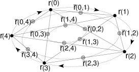
Figure 1: Schematic drawing of a set of periodic points with period 5 of a symplectic map with their midpoints.

As an example, consider the Arnol’d cat map. It is defined on a torus, ${\bf r}^{\prime\prime}=T{\bf r}^{\prime}(\hbox{mod}\,1)$, ${\bf r}\in[0,1)^{2}$, $T$ a $2\times 2$ matrix with integer coefficients. We choose the simplest combination that allows for quantization HB80 , $T=(2,1;3,2)$. The topology of the underlying classical space implies that both position and momentum be quantized, leading to a finite Hilbert-space dimension $D_{\cal{H}}$. The definition of the Wigner function can be adapted to this discrete periodic Hilbert space to avoid redundancies AB95 ; AD05 . In Fig. 2, we show the diagonal Wigner propagator after 1 and 3 iterations of the quantum map. The peaks of the diagonal propagator coincide perfectly with the periodic points of the classical map. Moreover, they appear with almost single-pixel precision. While the uncertainty relation requires a minimum area of $D_{\cal{H}}$ pixels, this is perfectly admissible for the propagator. To check Eq. (9), we compared the trace of the diagonal propagator to analytical results for $\sum_{j}N_{j}^{2}/|\hbox{det}\,(M_{j}-I)|$ (2.0 and 50.0, resp.), and found coincidence up to $6$ digits.

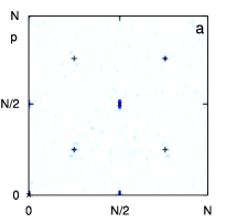
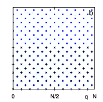
Figure 2: Diagonal Wigner propagator $G_{\rm W}({\bf r},n;{\bf r},0)$ for the quantized Arnol’d cat map at $n=1$ (a) and $n=3$ (b). Symbols $\times$, $+$ mark periodic points of the corresponding classical map and their midpoints, respectively (for better visibility of the data, symbols have been suppressed in the upper half of panel (b)). The Hilbert-space dimension is $D_{\cal{H}}=60$. Color code ranges from red (negative) to blue (positive).

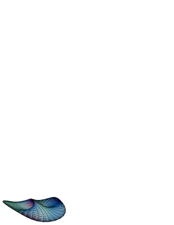
Figure 3: Surface formed by midpoints of a fictitious periodic orbit that is not circularly symmetric nor confined to a plane in phase space. It exhibits self-intersections but retains the topology of a closed two-dimensional ribbon, see text.

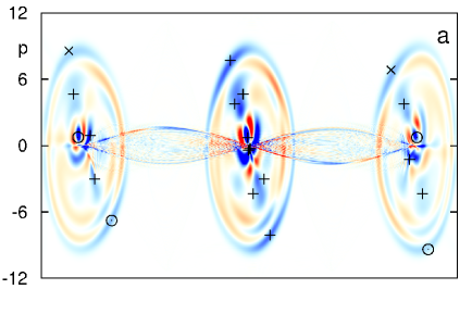
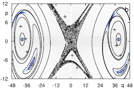
Figure 4: Diagonal Wigner (a) and Liouville (b) propagators $G({\bf r},t;{\bf r},0)$ for the harmonically driven quartic oscillator at $t=T\equiv 2\pi/\omega$, with $\omega_{0}=1.0$, $\omega=0.95$, $\phi=\pi/3$, $S=0.07$, and $E_{\rm b}=192.0$ (color code as in Fig. 2). For better orientation, we superimpose a stroboscopic surface of section of the same system (panel (b), black). The figure-$\infty$ structure is the Wigner caustic of a period-$T$ torus outside the frame shown (grey). Symbols $\odot$, $\times$ mark elliptic and hyperbolic periodic points of the classical system, resp., and $+$ their midpoints.

Going to systems in continuous time, a periodic orbit ${\bf r}_{j}(s)={\bf r}_{j}(s+T_{j})$ gives rise to midpoints $\bar{\bf r}_{j}(s^{\prime},s^{\prime\prime})=({\bf r}_{j}(s^{\prime})+{\bf r}_{j}(s^{\prime\prime}))/2$. This replaces Eq. (Time-domain scars: resolving the spectral form factor in phase space) with

$$G_{{\rm W}j}({\bf r}^{\prime\prime},t;{\bf r}^{\prime},0)=2\delta({\bf r}^{\prime\prime}-M_{j}{\bf r}^{\prime})\times$$

$$\cos\big{(}({\bf r}_{j}(s^{\prime\prime})-{\bf r}_{j}(s^{\prime}))\wedge({\bf r}^{\prime\prime}-{\bf r}^{\prime})/\hbar\big{)}\delta(t-T_{j}).$$ (10)

The midpoints now merge into a continuous two-dimensional surface ${\cal{S}}_{j}$ parameterized by $(s^{\prime},s^{\prime\prime})$, $0\leq s^{\prime},s^{\prime\prime}<T_{j}^{\rm p}$, the length of the orbit. Topologically it forms a closed ribbon. As a consequence, the diagonal propagator consists of a $\delta$-function only in the subspace orthogonal to ${\cal{S}}_{j}$, $G_{{\rm W}j}({\bf r},t;{\bf r},0)=\delta({\bf r}_{\perp})\delta(t-T_{j})/|\hbox{det}\,(M_{j\perp}-I)|$, where $M_{j\perp}$ is the stability matrix restricted to the $(2f-2)$-dimensional subspace ${\bf r}_{\perp}$. Upon tracing, the integration over ${\cal{S}}_{j}$ yields a factor ${T_{j}^{\rm p}}^{2}$, its effective area,

$$P_{{\rm ret}\,j}^{\rm qm}(t)=\Delta E\,{T_{j}^{\rm p}}^{2}\,\delta(t-T_{j})/2\pi\hbar|\hbox{det}\,(M_{j\perp}-I)|.$$ (11)

In Cartesian phase-space coordinates ${\bf r}$, ${\cal{S}}_{j}$ may have a nontrivial geometry. In general, it will exhibit a Wigner caustic ber76 , an overlap of three leaves near the center of the orbit, owing to the fact that a given point in this region may be the midpoint of more than one pair of periodic points on the orbit. The phenomenon can well be observed in Fig. 4. If the periodic orbit is not confined to a plane, this geometric degeneracy will be lifted, resulting in folds and self-intersections, illustrated in Fig. 3 for a fictitious periodic orbit.

A pertinent example is the harmonically driven quartic oscillator $H(p,q,t)=p^{2}/2m-m\omega_{0}^{2}q^{2}/4+m^{2}\omega_{0}^{4}q^{4}/64E_{\rm b}+Sq\cos(\omega t+\phi)$ GD&91 , with generally mixed phase space. In the diagonal propagator at $t=T\equiv 2\pi/\omega$ (Fig. 4) we identify a number of isolated peaks at periodic points of the classical dynamics, elliptic as well as hyperbolic, and their midpoints, and an enhancement over a well-defined region, to be interpreted as the Wigner caustic of a period-$T$ torus outside the frame shown, as confirms the coincidence with the corresponding classical feature in Fig. 4b.

Refinements and perspectives An alternative access to the Wigner propagator near periodic orbits is Berry’s scar function, a semiclassical approximation to the Weyl propagator in the energy domain ber89 . It responds to the special situation close to a periodic orbit $j$ by using local curvilinear coordinates: energy, time, and remaining phase-space directions ${\bf r}_{j\perp}$ perpendicular to the orbit. Transformed to the time domain and substituted for the Weyl propagator in Eq. (5), it leads to a semiclassical approximation for the diagonal Wigner propagator,

$$G_{{\rm W}j}({\bf r},t;{\bf r},0)=\frac{T_{j}^{\rm p}/2\pi\hbar}{|\hbox{det}\,(M_{j\perp}-I)|}\delta({\bf r}_{j\perp})\delta(t-T_{j}).$$ (12)

The primitive period $T_{j}^{\rm p}$ and the determinantal prefactor measure the length and the effective cross section, resp., of the “phase-space tube” around the orbit that contributes to the diagonal propagator. By contrast to Eq. (Time-domain scars: resolving the spectral form factor in phase space), the degeneracy factor $T_{j}^{\rm p}$ appears here already before tracing: The use of local coordinates condenses the contributions of periodic points as well as midpoints onto the orbit. Equation (12) does not apply outside the orbit $j$ and therefore does not allow for indiscriminate tracing over all of phase space.

The midpoint contribution to $G_{\rm W}({\bf r},t;{\bf r},0)$ giving rise to marked non-classical features is a manifestation of quantum coherence. It measures the quantum return probability for Schrödinger-cat states distributed over different points of the same periodic orbit. In the presence of incoherent processes, it decays on the dephasing timescale. The Wigner propagator, operating on the projective Hilbert space, readily permits including this effect zur01 and thus to identify exclusively the classical invariant manifolds, unaffected by the uncertainty relation, as peaks of a purely quantum-mechanical distribution. Phase-space features associated to non-diagonal contributions to the form factor will be even more elusive and geometrically more involved, but are in principle accessible to numerical study.

We have provided analytical and numerical evidence that Eq. (1) can be interpreted as a global relation between quantum and classical return probabilities which can be broken down into contributions of invariant phase-space manifolds. They enter with weight factors that measure the size of the set contributing coherently, and lead to important exceptions to Eq. (7). Analytical evidence based on presently available semiclassical approximations TDS06 indicates they are restricted to the diagonal ${\bf r}^{\prime}={\bf r}^{\prime\prime}$ (where they are least expected) and hence of measure zero. They are qualitatively different for integrable systems: In action-angle variables, the size of the degenerate sets is independent of time dit96 and therefore does not contribute an extra factor $t$. This in turn reflects the different dimensions and topologies of periodic tori vs. isolated unstable periodic orbits, indicating how to generalize this to more involved cases like systems with mixed phase space. Merging the different contributions on the classical side into more global quantities like the Frobenius-Perron modes AA&96 remains as a challenge for future research.

Fruitful discussions with D. Braun, F. Haake, H. J. Korsch, A. M. Ozorio de Almeida, T. H. Seligman, M. Sieber, U. Smilansky, R. Vallejos, and financial support by Colciencias, U. Nal. de Colombia, and VolkswagenStiftung are acknowledged with pleasure. We enjoyed the hospitality extended to us by CBPF (Rio de Janeiro), CIC (Cuernavaca), MPIPKS (Dresden), and U. of Technology Kaiserslautern.

References

- [1] M. C. Gutzwiller. J. Math. Phys., 12:343, 1971.
- [2] E. J. Heller. Phys. Rev. Lett., 53:1515, 1984.
- [3] F. Toscano et al. Phys. Rev. Lett., 86:59, 2001.
- [4] M. Sieber et al. Physica Scripta, T90:128, 2001.
- [5] S. Müller et al. Phys. Rev. Lett., 93:014103, 2004.
- [6] T. Dittrich and U. Smilansky. Nonlinearity, 4:85, 1991.
- [7] T. Dittrich. Phys. Rep., 271:267, 1996.
- [8] P. P. de M. Rios et al. J. Phys. A, 35:2609, 2002.
- [9] T. Dittrich et al. Phys. Rev. Lett., 96:070403, 2006.
- [10] M. Saraceno. Ann. Phys. (NY), 199:37, 1990.
- [11] F. McLafferty. J. Chem. Phys., 78:3253, 1983.
- [12] J. H. Hannay and M. V. Berry. Physica, 1D:267, 1980.
- [13] O. Agam and N. Brenner. J. Phys. A, 28:1345, 1995.
- [14] A. Argüelles and T. Dittrich. Physica A, 356:72, 2005.
- [15] M. V. Berry. Phil. Trans. Roy. Soc. A, 387:237, 1976.
- [16] F. Grossmann et al. Phys. Rev. Lett., 67:516, 1991.
- [17] M. V. Berry. Proc. Roy. Soc. Lond. A, 423:219, 1989.
- [18] W. H. Zurek. Nature, 412:712, 2001.
- [19] A. V. Andreev et al. Phys. Rev. Lett., 76:3947, 1996.