Prompt high-energy emission from gamma-ray bursts in the internal shock model

Abstract

Context. Gamma-ray bursts (GRB) are powerful, short duration events with a spectral luminosity peaking in the keV - MeV (BATSE) range . The prompt emission is thought to arise from electrons accelerated in internal shocks propagating within a highly relativistic outflow.

Aims. The launch of Fermi offers the prospect of observations with unprecedented sensitivity in high-energy (HE, $>$100 MeV) gamma-rays. The aim is to explore the predictions for HE emission from internal shocks, taking into account both dynamical and radiative aspects, and to deduce how HE observations constrain the properties of the relativistic outflow.

Methods. The prompt GRB emission is modelled by combining a time-dependent radiative code, solving for the electron and photon distributions, with a dynamical code giving the evolution of the physical conditions in the shocked regions of the outflow. Synthetic lightcurves and spectra are generated and compared to observations.

Results. The HE emission deviates significantly from analytical estimates, which tend to overpredict the IC component, when the time dependence and full cross-sections are included. The exploration of the parameter space favors the case where the dominant process in the BATSE range is synchrotron emission. The HE component becomes stronger for weaker magnetic fields. The HE lightcurve can display a prolonged pulse duration due to IC emission, or even a delayed peak compared to the BATSE range. Alternatively, having dominant IC emission in the BATSE range requires most electrons to be accelerated into a steep power-law distribution and implies strong second order IC scattering. In this case, the BATSE and HE lightcurves are very similar.

Conclusions. The combined dynamical and radiative approach allows a firm appraisal of GRB HE prompt emission. A diagnostic procedure is presented to identify from observations the dominant emission process and derive constrains on the bulk Lorentz factor, particle density and magnetic field of the outflow.

1 Introduction

The forthcoming first results of the Fermi gamma-ray space telescope call for a detailed study of the high energy (above 100 MeV) gamma–ray burst (GRB) emission. Current observational information on very high-energy gamma–rays emitted in a GRB date from the EGRET (Energetic Gamma–Ray Experiment Telescope) mission on board the CGRO (Compton Gamma Ray Observatory). It detected high energy photons from a handful of GRBs; the most energetic (18 GeV) photon was detected in the case of GRB 940217 (Hurley et al. 1994). González et al. (2003) reported the observation of a bright high-energy component in GRB 941017, showing a strong temporal evolution, distinct from the low-energy ($<$2 MeV) component. The inspection of the sample of gamma–ray bursts that were observed both by EGRET and BATSE (Burst and Transient Source Experiment) indicates that these bursts were among the brightest ones detected by BATSE (e.g. Baring 2006); as BATSE trigger was sensitive in the lower energy range, there could be a population of bursts with high energy photons that did not trigger BATSE (Jones et al. 1996). Kaneko et al. (2008) reported the spectral analysis of combined BATSE and EGRET data for 15 bright GRBs in energy range $\sim$30 keV-200 MeV, emphasizing the importance of such broadband spectral analysis in constraining the high-energy spectral indices and break energies of GRBs that have significant MeV emission. More recently Giuliani et al. (2008) reported observations of GRB 080514B by AGILE showing some evidence that the emission above 30 MeV extends for a longer duration than the emission observed at lower energies. Evidence of even higher (TeV) energy emission from GRBs was reported from ground-based experiments, based on the detection of extensive air showers produced by high energy photons propagating in the atmosphere (Atkins et al. 2000).

The observation of high energy spectral components in GRBs can provide strong constraints on present models for the GRB prompt phase. GRBs are believed to be produced by ultra-relativistic ($\Gamma\ga 100$) outflows ejected from a newly formed compact stellar mass source. The prompt gamma-ray emission is usually interpreted as radiation from accelerated electrons in shock waves that propagate within the outflow (Rees & Mészáros 1994). Such internal shocks can form if the ejection process by the central source is highly variable. A high energy spectral component is expected within this framework (see e.g. Papathanassiou & Mészáros 1996; Sari & Piran 1997; Pilla & Loeb 1998; Guetta & Granot 2003; Pe’er & Waxman 2004; Razzaque et al. 2004; Asano & Inoue 2007; Gupta & Zhang 2007; Galli & Guetta 2008; Fan & Piran 2008; Ando et al. 2008). The typical GRB spectrum in the low gamma-ray range, as observed for instance by BATSE, is a smoothly connected broken power law with a break energy in the range 0.1 - 1 MeV. This component can be directly produced by synchrotron radiation from the shock accelerated electrons, or by inverse Compton scatterings of low-energy synchrotron photons by the relativistic electrons. Thus observations of the GRB spectrum extending to very high energy emission (GeV ranges) can be expected when the keV-MeV photons are inverse Compton scattered (provided that the $\gamma\gamma$ opacity in the source is low). Depending on the relevant parameters, the flux of the high energy component can be even comparable to the prompt GRB gamma–ray flux in BATSE energy range.

Significant observational progress is expected with the launch of Fermi, whose two instruments, GBM (GLAST burst monitor) and LAT (Large Array Telescope) will allow the observation of GRBs in an unprecedented spectral range from 8 keV to 10 GeV or above (Gehrels & Michelson 1999). The LAT has a large field of view ($\sim 2\ \mathrm{sr}$), is about 10 times more sensitive than EGRET and has a very short dead time of $\sim 100\,\mathrm{\mu s}$ (compared to 100 ms for EGRET). Fermi should therefore detect 100 to 200 GRBs per year (GBM+LAT), with an appreciable number of them being bright enough above 100 MeV to allow a good characterization of their temporal and spectral properties in the high-energy gamma-ray range.

This paper presents a detailed calculation of the GRB prompt emission in the context of the internal shock model, focussing on the high energy (above 100 MeV) range. The emission in the shocked region is computed using a radiative code that was developed to solve simultaneously the time evolution of the electron and photon distribution, which is a significant improvement compared to studies based on an analytical estimate of the spectrum. This radiative calculation is less detailed than in previous studies (Pe’er & Waxman 2005; Asano & Inoue 2007) as it does not include components emitted by shock-accelerated protons or by electron–positron pairs created from $\gamma\gamma$ annihilation. However it includes all the relevant processes for the emission from shock-accelerated electrons, whose contribution is expected to be dominant. In addition, this radiative calculation is combined for the first time with a detailed dynamical simulation of the internal shock phase, which allows us not only to estimate the spectrum of the prompt GRB emission, but to generate full synthetic GRBs with lightcurves and spectra. This approach is described in Sect. 2. The effect of the parameters describing the physical conditions in the shocked medium on the shape of the emitted spectrum in the comoving frame is shown in Sect. 3. The parameter space of the internal shock model is explored in a systematic way in Sect. 4, which allows the identification of the different classes of high-energy spectra that can be expected. We show how Fermi data will allow us to diagnose the dominant radiative process (synchrotron radiation vs inverse Compton scatterings), the physical conditions in the shocked medium (electron distribution, magnetic field) and the properties of the relativistic outflow (Lorentz factor and injected kinetic power). Finally, Sect. 5 describes examples of synthetic bursts (lightcurves and spectra) and discuss how the comparison between the LAT and the GBM lightcurves and the observed spectral evolution in Fermi bursts are also powerful tools to better constrain the physical processes at work in GRBs. Sect. 6 summarizes the results of this study.

2 Internal shocks: dynamics and radiative processes

We assume that a relativistic outflow is ejected by the central source of the gamma-ray burst, and that, due to initial variability in the distribution of the Lorentz factor, shock waves form and propagate within this outflow (internal shocks, Rees & Mészáros 1994). A fraction of the kinetic energy which is dissipated in the shock waves is radiated and produces the observed prompt GRB. Here, we focus on the most discussed version of the internal shock model, where the radiation is due to shock-accelerated electrons in optically thin conditions. It has been suggested that shock accelerated protons could also contribute to the high-energy emission (Razzaque et al. 2004; Asano & Inoue 2007; Asano et al. 2008), or that the emission could occur in optically thick regions leading to quasi-thermal comptonization (Ghisellini & Celotti 1999; Mészáros & Rees 2000; Pe’er & Waxman 2004; Giannios & Spruit 2007), or that the dominant process is not related to shock-accelerated electrons but rather to decaying pions (Paczynski & Xu 1994). These alternative possibilities are not considered in this paper.

In order to follow the time evolution of the photon spectrum emerging from the relativistic outflow during the internal shock phase, several steps are needed:

1. The dynamics of the internal shock phase must be followed to determine the physical conditions behind each shock wave;

2. In the shocked medium, electrons are accelerated and the magnetic field is amplified. The emitted photon spectrum has to be computed from the time-dependent evolution of the relativistic electrons. This evolution is governed by several radiative processes that are in competition with the adiabatic cooling due to the spherical expansion.

3. From the evolution of the emission in the comoving frame of the shocked material, one can deduce the observed prompt GRB lightcurve and spectrum.

Some aspects of this project have already been studied by several authors, who focus on the second step (radiative processes in the comoving frame) after assuming a typical collision between two relativistic shells for the first step. This has been done either using an approximate analytical or semi–analytical estimate of the spectrum (e.g. Papathanassiou & Mészáros 1996; Guetta & Granot 2003; Gupta & Zhang 2007; Galli & Guetta 2008; Fan & Piran 2008; Ando et al. 2008) or a detailed radiative code (Pe’er & Waxman 2004; Asano & Inoue 2007). Such studies allow to discuss different emission mechanisms of high energy photon production during internal shocks and to derive the expected high energy photon spectrum from one single shocked relativistic shell. However, they cannot produce full lightcurves and time-evolving spectra, and evaluate the role of the dynamics of internal shocks in the observed spectral evolution. In this work we attempt to improve this approach by combining a complete model for the dynamics of the internal shocks with a detailed calculation of the relevant radiative processes occurring in the shocked medium. This allows us for the first time to obtain the time evolution of the high-energy gamma-ray emission in a GRB. The procedure we have adopted in described in the present section.

2.1 Dynamical evolution during the internal shock phase

The dynamics of internal shocks within a relativistic outflow has been described in Kobayashi et al. (1997) in the case where the central engine is emitting a discrete number of shells, separated by short periods without any ejection. In this scenario, each pulse observed in the GRB lightcurve is due to a collision between two shells. One potential problem with this approach is that the pulse shape in the decay phase is dominated by the so-called curvature effect, i.e. the spreading of the arrival time of photons emitted simultaneously on a curved surface. Such a decay is too fast compared to observations (see e.g. Soderberg & Fenimore 2001). In this paper, the dynamics of internal shocks is rather computed using the model developed by Daigne & Mochkovitch (1998), where the relativistic ejection is now considered as a continuous process. Instead of collisions between discrete shells, internal shocks are in this case shock waves propagating within the outflow. In the observed lightcurve, the shape of pulses in their decay phase is then determined by the hydrodynamical timescale associated with the propagation of the shock waves, rather than the curvature effect (except at the very end of this dynamical phase). Slow pulse decays can easily be obtained, which greatly improves the agreement with observations (Daigne & Mochkovitch 2003).

Figure 1: Dynamics of internal shocks: an example. Left. Evolution of the distribution of the Lorentz factor in the relativistic outflow. In this example, the initial distribution (thick solid line) corresponds to a case where material has been ejected for $t_{\mathrm{w}}=$ 2 s by the central source, with a Lorentz factor $\Gamma(t)$ increasing from 100 to 400. Two internal shock waves form when the faster part catches up with the slower one, as it is shown by the evolution of the distribution of the Lorentz factor with time (thin solid lines). The dynamics is computed assuming an injected kinetic power $\dot{E}=5\times 10^{52}\ \mathrm{erg\leavevmode\nobreak\ s^{-1}}$. Right. Corresponding physical conditions ($\Gamma_{*}$, $\rho_{*}$ and $\epsilon_{*}$) in the shocked material (see text), plotted as a function of the photon arrival time. For each curve, the two branches correspond to the two shock waves that form in the outflow. Two additional quantities are also plotted, $\Gamma_{\mathrm{m}}$ and $B^{\prime}$, assuming $\epsilon_{\mathrm{e}}=1/3$, $\zeta=10^{-2}$, $p=2.5$ and $\epsilon_{\mathrm{B}}=1/3$. Circles indicate the physical conditions at times $t=6.9\times 10^{3}$, $1.9\times 10^{4}$, $5.2\times 10^{4}$ and $1.8\times 10^{5}\ \mathrm{s}$, for which the Lorentz factor distribution in the outflow is plotted in the left panel. Notice that the shock propagating forward reaches rapidly the front edge so that, in this example, the emission will be dominated by one shock wave only. This example will lead to a single pulse burst. In practice, the initial Lorentz factor considered here has to be seen as a building block for more realistic distributions leading to multi-pulse lightcurves (see Sect. 5.2).

The dynamics during the internal shock phase is entirely determined from the following parameters : the total duration $t_{\mathrm{w}}$ of the relativistic ejection and the history of the Lorentz factor $\Gamma(t)$ and of the injected kinetic power $\dot{E}(t)$ during this ejection. In practice, the outflow is described as a series of shells emitted regularly over a timescale $\Delta t\ll t_{\mathrm{w}}$, so that the number of shells is much larger that the number of pulses in the lightcurve. These shells interact only by direct collisions, so that the propagation of a shock wave is discretized by a succession of shocks between shells. The details of the implementation of this model are described in Daigne & Mochkovitch (1998). This method has been validated by a comparison with the results of a 1D Lagrangian relativistic hydrocode (Daigne & Mochkovitch 2000). Relativistic hydrodynamical simulations of internal shocks have also been performed by Mimica et al. (2004) in the context of blazars and by Mimica et al. (2007) in the context of GRBs. The authors discuss the efficiency of the conversion of kinetic energy into radiation, and especially the impact of the possible magnetization of the outflow, which is not considered in the present paper. The output of a simulation of the internal shock dynamics is the time evolution of the physical conditions in the shocked medium behind each shock wave (comoving mass density $\rho_{*}$, comoving specific energy density $\epsilon_{*}$, and Lorentz factor $\Gamma_{*}$). This is illustrated in a simple example shown in Fig. 1, where the Lorentz factor distribution in the outflow is plotted at different times $t$, and the physical conditions in the shocked medium are plotted as a function of $t_{\mathrm{obs}}/(1+z)=t-R/c$ (arrival time in the observer frame of photons emitted along the line of sight at radius $R$ and time $t$).

To estimate the typical radius and shock conditions in internal shocks, a simple “two shells” model is often used (see e.g. Rees & Mészáros 1994; Barraud et al. 2005; Daigne & Mochkovitch 2007; Kumar & McMahon 2008). We consider the ejection of two equal mass relativistic shells with Lorentz factor $\Gamma_{1}$ and $\Gamma_{2}$ from the central source. Shell 1 is ejected first and shell 2 after shell 1, with a delay $\tau$. If the contrast $\kappa=\Gamma_{2}/\Gamma_{1}$ is greater than unity, an internal shock will occur at a radius

$$R_{\mathrm{is}}\simeq\frac{8\kappa^{2}}{(\kappa-1)(\kappa+1)^{3}}\bar{\Gamma}^{2}c\tau\ ,$$ (1)

where the average Lorentz factor is $\bar{\Gamma}=(\Gamma_{1}+\Gamma_{2})/2$. The fraction of the kinetic energy of the shells which is dissipated in the collision is

$$f_{\mathrm{dyn}}\simeq\frac{\left(\sqrt{\kappa}-1\right)^{2}}{\kappa+1}\ .$$ (2)

Then, if the injected kinetic power during the relativistic ejection phase is $\dot{E}$, the Lorentz factor, comoving mass density and comoving specific internal energy density in the shocked material are given by

$$\Gamma_{*} \simeq \frac{2\sqrt{\kappa}}{1+\kappa}\bar{\Gamma}\ ,$$

$$\rho_{*} \simeq \frac{\dot{E}}{4\pi R_{\mathrm{is}}^{2}\Gamma_{*}^{2}c^{3}}\ ,$$

$$\epsilon_{*} \simeq \frac{\left(\sqrt{\kappa}-1\right)^{2}}{2\sqrt{\kappa}}c^{2}\ .$$ (3)

These simple scaling laws will be used to explore the parameter space of the internal shock model in the next section.

Once the dynamics of the internal shock phase is well understood and the physical conditions in the shocked material are known, more assumptions are necessary to compute the emission. This is described in the next subsection.

2.2 Physical conditions in the shocked medium

The physics of the acceleration of particles in relativistic shock waves, as well as the amplification of the magnetic field, is far from being fully understood. It is therefore impossible in our state of knowledge to directly estimate the electron distribution and the magnetic field in the shocked medium from $\Gamma_{*}$, $\rho_{*}$ and $\epsilon_{*}$ using first principles. Therefore, the microphysics related to these processes is usually parameterized in a very simple way, which is adopted in the present paper: (i) it is assumed that a fraction $\epsilon_{\mathrm{e}}$ of the dissipated energy is injected in a fraction $\zeta$ of the ambient electrons that are accelerated to relativistic energies, with a power-law distribution of slope $-p$. Note that most GRB studies (prompt and afterglow emission modelling) are restricted to the case $\zeta=1$ (all electrons are accelerated) but numerical simulations of particle acceleration in relativistic shocks suggest that it may not be the case (see e.g. Bykov & Mészáros 1996; Eichler & Waxman 2005; Spitkovsky 2008); (ii) it is assumed that a fraction $\epsilon_{\mathrm{B}}$ of the dissipated energy is injected in the magnetic field. We do not investigate in this paper an alternative scenario, where the magnetic field is dominated by a large-scale component anchored in the central source (see e.g. Spruit et al. 2001). With these four additional parameters ($\epsilon_{\mathrm{e}}$, $\zeta$, $p$ and $\epsilon_{\mathrm{B}}$), the number density of non-thermal electrons can be computed

$$n^{\mathrm{acc}}_{\mathrm{e}}\simeq\zeta\frac{\rho_{*}}{m_{\mathrm{p}}}\ ,$$ (4)

as well as their initial distribution

$$n\left(\gamma\right)\simeq(p-1)\frac{n^{\mathrm{acc}}_{\mathrm{e}}}{\Gamma_{\mathrm{m}}}\left(\frac{\gamma}{\Gamma_{\mathrm{m}}}\right)^{-p}\ \mathrm{for}\ \gamma\geq\Gamma_{\mathrm{m}}$$ (5)

with

$$\Gamma_{\mathrm{m}}\simeq\frac{p-2}{p-1}\frac{\epsilon_{\mathrm{e}}\ \rho_{*}\epsilon_{*}}{n^{\mathrm{acc}}_{\mathrm{e}}m_{\mathrm{e}}c^{2}}\simeq\frac{p-2}{p-1}\frac{\epsilon_{\mathrm{e}}}{\zeta}\frac{m_{\mathrm{p}}}{m_{\mathrm{e}}}\frac{\epsilon_{*}}{c^{2}}\ .$$ (6)

The magnetic field in the comoving frame of the shocked material is given by

$$B^{\prime}\simeq\sqrt{8\pi\epsilon_{\mathrm{B}}\ \rho_{*}\epsilon_{*}}\ .$$ (7)

The evolution of $\Gamma_{\mathrm{m}}$ and $B^{\prime}$ is plotted for our example in Fig. 1.

In practice, it is assumed that the relativistic electron distribution extends up to a maximum Lorentz factor $\Gamma_{\mathrm{M}}$, defined as the Lorentz factor where the acceleration timescale becomes comparable to the minimum of the radiative timescale and the escape timescale (see below). This corresponds to the most efficient acceleration that can be expected. In the comoving frame of the shocked region, the acceleration timescale of an electron with Lorentz factor $\gamma$ is estimated as $R^{\prime}_{\mathrm{L}}(\gamma)/c$, where

$$R^{\prime}_{\mathrm{L}}(\gamma)=\frac{\gamma m_{\mathrm{e}}c^{2}}{eB^{\prime}}$$ (8)

is the Larmor radius. This leads to

$$\Gamma_{\mathrm{M}}=\min{\left(\left(\frac{6\pi e}{\sigma_{\mathrm{T}}B^{\prime}}\right)^{1/2};\frac{eB^{\prime}t^{\prime}_{\mathrm{ex}}}{m_{\mathrm{e}}c}\right)}\ ,$$ (9)

where the radiative timescale is taken to be equal to the synchrotron timescale (Eq. (17) below) and the escape timescale is identified with the dynamical timescale $t^{\prime}_{\mathrm{ex}}$ (Eq. (10) below). Note that when inverse Compton losses are important, this expression overestimates the maximum Lorentz factor $\Gamma_{\mathrm{M}}$. This is further discussed later on.

2.3 Emission in the comoving frame

Timescales.

Two timescales are necessary to characterize the physics in the shocked region: (i) the dynamical timescale

$$t^{\prime}_{\mathrm{ex}}\simeq\frac{R}{\Gamma_{*}c}\ ,$$ (10)

which is the typical timescale associated with the adiabatic cooling due to the spherical expansion; and (ii) the radiative timescale $t^{\prime}_{\mathrm{rad}}$, defined as the timescale necessary for the relativistic electrons to radiate most of their energy. As described in Sari et al. (1998), electrons with $t^{\prime}_{\mathrm{rad}}\ll t^{\prime}_{\mathrm{ex}}$ are in “fast cooling” regime and will radiate efficiently, whereas electrons with $t^{\prime}_{\mathrm{rad}}\gg t^{\prime}_{\mathrm{ex}}$ are in “slow cooling” regime and will loose most of their energy via the adiabatic cooling. In internal shocks, the short variability timescale observed in the lightcurves imposes that all electrons are in fast cooling regime (Rees & Mészáros 1994; Sari et al. 1996; Kobayashi et al. 1997). This is also probably required by pure energetic considerations, as the huge gamma-ray luminosities observed in GRBs are very difficult to understand if electrons are not radiating efficiently. From a numerical point of view, the advantage of being in fast cooling regime is that the emission is produced over a short timescale: relativistic electrons accelerated in one collision will radiate most of their energy before the next collision occurs. This allows to compute the emission in an independent way: for each dynamical timestep (duration $\sim t^{\prime}_{\mathrm{ex}}$), the radiation in the shocked region is computed assuming that the dynamical quantities (e.g. the density) do not vary.

Geometry.

The shocked region is a shell with radius $R$, opening angle $\Delta\theta$ (equal to the opening angle of the outflow, that can be considered as constant in the internal shock phase, the lateral expansion becoming efficient only when the outflow has notably decelerated) and comoving width $\Delta^{\prime}\sim ct^{\prime}_{\mathrm{ex}}$. During the dynamical timescale $t^{\prime}_{\mathrm{ex}}$, the emission in the comoving frame can be computed assuming constant dynamical quantities. The causally connected region during this duration has a size $ct^{\prime}_{\mathrm{ex}}$ which is small compared to the lateral size of the shell $R\Delta\theta$, as long as $\Delta\theta\gg 1/\bar{\Gamma}$. In the comoving frame of the shocked region, one can therefore neglect the curvature and consider a infinite plane layer with width $ct^{\prime}_{\mathrm{ex}}$.

As electrons are in fast cooling regime with $t^{\prime}_{\mathrm{rad}}\ll t^{\prime}_{\mathrm{ex}}$, most of the evolution occurs on a short timescale, corresponding to a causally connected region of size $ct^{\prime}_{\mathrm{rad}}$ much smaller than the physical width of the region. Therefore, it is justified to assume that, if the shell is initially homogeneous, it will remain so for most of the evolution: the density distribution of electrons will depend on time, but not on the position in the shocked region. The same will happen for the photon distribution, which will appear as isotropic everywhere in the shocked region. This is of course not strictly valid within a distance $ct^{\prime}_{\mathrm{rad}}$ from the edge of the shell, but the corresponding volume is negligible, as $t^{\prime}_{\mathrm{rad}}\ll t^{\prime}_{\mathrm{ex}}$.

The photon field

At time $t^{\prime}=0$, just after the collision, when the particle acceleration and the amplification of the magnetic field are achieved (it is assumed that these processes operate on timescales which are short compared to the radiative and the dynamical timescales), the electron distribution is given by Eq. (5) and the photon density is zero. This is justified as all electrons that were shock-accelerated earlier have already cooled.

The photon density distribution at time $t^{\prime}$ at a given position in the shocked region is given by

$$n_{\nu^{\prime}}(t^{\prime})=\frac{4\pi}{c}\frac{I_{\nu^{\prime}}(t^{\prime})}{h\nu^{\prime}}\ ,$$ (11)

due to the isotropy of the photon field (see above). If absorption is neglected at this stage of the discussion, the specific intensity $I_{\nu^{\prime}}(t^{\prime})$ is built by integration of

$$\frac{dI_{\nu^{\prime}}}{ds^{\prime}}=j_{\nu^{\prime}}$$ (12)

along a ray, from $s^{\prime}=0$ to $s^{\prime}=ct^{\prime}$ (where $s^{\prime}=0$ is the position where $n_{\nu^{\prime}}$ is computed), due to the finite speed of light. Assuming an isotropic emission by electrons, this leads to

$$I_{\nu^{\prime}} = \frac{1}{4\pi}\int_{0}^{ct^{\prime}}ds^{\prime}P_{\nu^{\prime}}\left(s^{\prime},\tilde{t}^{\prime}=t^{\prime}-\frac{s^{\prime}}{c}\right)$$ (13)

$$= \frac{c}{4\pi}\int_{0}^{t^{\prime}}\ d\tilde{t}^{\prime}P_{\nu^{\prime}}(\tilde{t}^{\prime})\ ,$$

where the homogeneity of the shock region is taken into account (see above). Finally, the photon density distribution is given by

$$n_{\nu^{\prime}}(t^{\prime})=\int_{0}^{t^{\prime}}d\tilde{t}^{\prime}\frac{P_{\nu^{\prime}}(\tilde{t}^{\prime})}{h\nu^{\prime}}\ ,$$ (14)

where it appears clearly that the local photon field is built by accumulating photons coming from a growing region of size $c\tilde{t}^{\prime}$ and therefore depends on the whole history of the emission between $\tilde{t}^{\prime}=0$ and $\tilde{t}^{\prime}=t^{\prime}$. In the next paragraph this equation is expanded by giving explicitly the emission processes that are considered in the present study and including the absorption processes that were neglected in this paragraph.

Radiative processes.

Many radiative processes can operate in the shocked medium. In this paper, we focus on the processes that are expected to be dominant if the radiation is mainly produced by electrons, i.e. we do not include contributions associated to a possible population of relativistic protons accelerated in the shock. Such a component is included in the calculations made by Asano & Inoue (2007) for a typical shock. Their results show that (i) for most parameters, the proton contribution is negligible, especially below a few GeV; (ii) it is only when $\epsilon_{\mathrm{B}}\gg\epsilon_{\mathrm{e}}$, i.e. when most of the dissipated energy is injected in the magnetic field and in protons, rather than in electrons, that a non negligible proton component emerges.

Accelerated relativistic electrons in the amplified magnetic field will radiate via the synchrotron process. These synchrotron photons can be scattered to higher energies by relativistic electrons (inverse Compton). At low energy, they can also be absorbed (synchrotron-self absorption). At high energies, photon–photon annihilation can occur, producing electron-positron pairs. The corresponding pairs could contribute to the radiation, but this contribution is not considered in the present paper, as we limit our studies to cases where the production of pairs is weak (see next section). We did not consider in this study the case of the “jitter radiation” (Medvedev 2000; Medvedev & Spitkovsky 2008) that is an alternative to the standard synchrotron radiation.

Based on the timescales and the geometry discussed above, we have implemented a radiative code to solve the evolution of electrons and photons in the comoving frame of the shocked medium during a dynamical timestep. Two equations are solved, one for the evolution of the comoving electron density distribution $n\left(\gamma,t^{\prime}\right)$ :

$$\frac{\partial n}{\partial t^{\prime}}=-\frac{\partial}{\partial\gamma}\left[\left.\frac{d\gamma}{dt^{\prime}}\right|_{\mathrm{syn+ic+ad}}n\left(\gamma,t^{\prime}\right)\right]$$ (15)

and one for the evolution of the comoving photon density distribution $n_{\nu^{\prime}}(t^{\prime})$ :

$$\frac{\partial n_{\nu^{\prime}}}{\partial t^{\prime}} = \int d\gamma\ n\left(\gamma,t^{\prime}\right)\frac{P_{\nu^{\prime}}^{\mathrm{syn+ic}}(\gamma)}{h\nu^{\prime}}$$ (16)

$$-cn_{\nu^{\prime}}(t^{\prime})\int d\gamma\ n\left(\gamma,t^{\prime}\right)\sigma_{\mathrm{sa}}\left(\gamma,\nu^{\prime}\right)$$

$$-cn_{\nu^{\prime}}(t^{\prime})\int d\tilde{\nu}^{\prime}\ n_{\tilde{\nu}^{\prime}}(t^{\prime})\sigma_{\gamma\gamma}\left(\nu^{\prime},\tilde{\nu}^{\prime}\right)\ .$$

The indexes $\mathrm{syn}$, $\mathrm{ic}$, $\mathrm{ad}$, $\mathrm{sa}$ and $\mathrm{\gamma\gamma}$ stand respectively for the following processes: synchrotron radiation, inverse Compton scattering, adiabatic cooling, synchrotron self-absorption and photon–photon annihilation.

The expressions of the different terms appearing in Eqs. (15) and (16) are listed in appendix A and the numerical method to solve this set of equations is described in appendix B. The adiabatic losses are estimated by $\left.d\gamma/dt^{\prime}\right|_{\mathrm{ad}}=-\gamma/t^{\prime}_{\mathrm{ex}}$. The synchrotron radiation is computed exactly, assuming an isotropic distribution of the pitch angle $\alpha$ between the electron velocity and the magnetic field. The synchrotron self-absorption is also computed using the exact cross-section (see e.g. Rybicki & Lightman 1979). Note that the corresponding heating term at low energy is neglected in Eq. (15). Inverse Compton scatterings are computed using the approximate kernel derived by Jones (1968), which is a very good approximation, even in the Klein-Nishina regime. Note that Eq. (16) does not include the loss term at low frequency corresponding to the source term at high energy. This is because the Thomson optical depth is always low in our case (see next section). We do not examine situations where comptonization could occur. Finally, the full cross-section for gamma-gamma annihilation is used, assuming an isotropic photon field (Gould & Schréder 1967). As mentioned above, the present version of the code does not include the associated pair creation term, so that we limit the study to cases where it is negligible (see next section).

Figure 2: Emission in the comoving frame: an example. This figure shows the result of the radiative calculation in the comoving frame of the shocked material, at time $1.9\times 10^{4}\ \mathrm{s}$ in the example shown in Fig. 1. Left. Evolution of the relativistic electron population. The initial distribution is plotted with a thick line. Right. Evolution of the photon spectrum $\left.\nu^{\prime}\right.^{2}n_{\nu^{\prime}}$. The final spectrum at $t^{\prime}=t^{\prime}_{\mathrm{ex}}$ is plotted with a thick line. Several phases are well identified: the synchrotron spectrum is built very early (thin solid line). Once these seed photons are present, inverse Compton scatterings produce high energy emission (dotted line). At late times, high-energy photons annihilate which reduces the intensity of the second peak in the spectrum (dashed line). The microphysics parameters are $\epsilon_{\mathrm{e}}=1/3$, $\zeta=10^{-2}$, $p=2.5$ and $\epsilon_{\mathrm{B}}=1/3$ so that the initial Thomson optical depth is $\tau_{\mathrm{T}}^{\mathrm{acc}}\simeq 6\times 10^{-5}$ and the critical Lorentz factor equals $\Gamma_{\mathrm{c}}\simeq 2.4$ (see text).

Following Sari et al. (1998), it is convenient to define $\Gamma_{\mathrm{c}}$ as the Lorentz factor of electrons whose synchrotron timescale

$$t_{\mathrm{syn}}^{\prime}\left(\gamma\right)=\frac{6\pi m_{\mathrm{e}}c}{\sigma_{\mathrm{T}}\left.B^{\prime}\right.^{2}\gamma}$$ (17)

is equal to the adiabatic cooling timescale, i.e.

$$\Gamma_{\mathrm{c}}=\frac{6\pi m_{\mathrm{e}}c}{\sigma_{\mathrm{T}}\left.B^{\prime}\right.^{2}t^{\prime}_{\mathrm{ex}}}\ .$$ (18)

When the synchrotron process is dominant, electrons with $\gamma>\Gamma_{\mathrm{c}}$ are in fast cooling regime. When inverse Compton scatterings become efficient, the effective transition between slow and fast cooling occurs at a Lorentz factor lower than $\Gamma_{\mathrm{c}}$ as the radiative timescale becomes shorter than the synchrotron timescale.

The solution at $t^{\prime}=t^{\prime}_{\mathrm{ex}}$ of system of Eqs. (15) and (16) is entirely determined by the expansion timescale $t^{\prime}_{\mathrm{ex}}$, the shape of the initial electron distribution (i.e. mainly $\Gamma_{\mathrm{m}}$ and $p$), the relativistic electron density $n_{\mathrm{e}}^{\mathrm{acc}}$ and the magnetic field $B^{\prime}$. Rather than using these two last quantities, it is convenient to consider alternatively the critical Lorentz factor $\Gamma_{\mathrm{c}}$ and the initial Thomson optical depth associated to relativistic electrons

$$\tau^{\mathrm{acc}}_{\mathrm{T}}=\sigma_{\mathrm{T}}n^{\mathrm{acc}}_{\mathrm{e}}ct^{\prime}_{\mathrm{ex}}\ .$$ (19)

The radiative calculation has to be made for each collision occurring in the dynamical phase, i.e. at each instant along the propagation of a shock wave within the relativistic outflow. Fig. 2 shows one of these elementary calculations. This case has been selected as the effect of each process is clearly identified (see caption of the figure). Possible additional effects (scatterings or absorption) between photons emitted in a shocked region and electrons or photons present in another shocked region, which could affect the high-energy spectrum (Gruzinov & Mészáros 2000), are not considered in the present paper but will be investigated in the future. We also ignore the effects of triplet pair production which can occur when electrons of very high energies encounter soft photons : the cross-section for this process becomes larger than the inverse Compton cross-section in the deep Klein-Nishina regime, for $\gamma\epsilon\ga 250$, where $\gamma$ is the electron Lorentz factor and $\epsilon=h\nu/m_{e}c^{2}$ the soft photon energy (Mastichiadis 1991). Finally, we do not include the possible interaction of the prompt gamma-rays emitted from internal shocks and the circumburst environment, that could also lead to an additional early high-energy component (Beloborodov 2002, 2005).

2.4 Observed flux

Once the emission in the comoving frame is computed at each instant along the propagation of internal shocks within the relativistic outflow, the observed flux as a function of time is computed by summing up the contributions of all shock waves, taking into account : (i) the relativistic effects (Lorentz transformation from the comoving frame of the shocked region to a fixed frame); (ii) the curvature of the emitting surface; (iii) the cosmological effects due to the redshift of the GRB source. The two first points require an integration over equal-arrival times surfaces, that is carried out following equations given in Woods & Loeb (1999). Any absorption in the gamma-ray range due to pair creation on the extragalactic background light is neglected. This would be important, depending on the redshift, above $\sim 10\,\mathrm{GeV}$. Examples of synthetic lightcurves and spectra produced following the complete procedure described in this section are presented in Sect. 5.

3 The emitted spectrum in the comoving frame

As described in Sect. 2, the emitted spectrum in the comoving frame of the shocked material is entirely determined by four parameters: (i) the magnetic field $B^{\prime}$; (ii) the adiabatic cooling timescale $t_{\mathrm{ex}}^{\prime}$; (iii) the relativistic electron density $n_{\mathrm{e}}^{\mathrm{acc}}$, and (iv) the shape of the initial distribution of the Lorentz factor of accelerated electrons, i.e. the slope $p$ and the minimum Lorentz factor $\Gamma_{\mathrm{m}}$ for a power-law distribution. A clear insight in the way that every of these parameters affects the radiative processes is necessary to anticipate the characteristics of the photon spectrum resulting from the shock-accelerated electrons.

The final observed photon spectrum comprises the contributions of all the photons emerging from the collisions occurring during the evolution of the relativistic outflow. We focus first on the radiative processes and the photon spectrum occurring after a single collision only and will describe later (§ 5) the complete GRB lightcurve and spectrum.

We have carried out spectral calculations corresponding to a large exploration of the parameter space $\left(B^{\prime},t^{\prime}_{\mathrm{ex}},n_{\mathrm{e}}^{\mathrm{acc}},\Gamma_{\mathrm{m}}\right)$ describing the physical conditions in the shocked material, assuming a fixed electron slope $p=2.5$. We computed 2744 spectra corresponding to : (i) 7 values of the magnetic field $\log{\left(B^{\prime}/1\ \mathrm{G}\right)}=1$, $1.5$, $2$, $2.5$, $3$, $3.5$ and $4$; (ii) 7 values of the dynamical timescale $\log{\left(t^{\prime}_{\mathrm{ex}}/1\ \mathrm{s}\right)}=0$, $0.5$, $1$, $1.5$, $2$, $2.5$ and $3$; (iii) 7 values of the electron density $\log{\left(n_{\mathrm{e}}^{\mathrm{acc}}/1\ \mathrm{cm^{-3}}\right)}=4$, $5$, $6$, $7$, $8$, $9$ and $10$; (iv) and 8 values of the minimum electron Lorentz factor $\log{\Gamma_{\mathrm{m}}}=1.5$, $2$, $2.5$, $3$, $3.5$, $4$, $4.5$ and $5$.

Figure 3: Radiative efficiency. The explored region of the parameter space of internal shocks is shown in the plane $u_{\mathrm{ic}}/u_{\mathrm{syn}}$ versus $\Gamma_{\mathrm{m}}/\Gamma_{\mathrm{c}}$ (shaded region labeled ’All’). The x-axis quantity measures the efficiency of inverse Compton scatterings and the y-axis compares the synchrotron and the adiabatic cooling timescales. Radiatively efficient cases, i.e. cases where most of the energy initially injected in relativistic electrons is radiated (see text) are indicated (shaded region labeled ’Rad. efficient’). Inverse Compton scatterings reduce the effective radiative timescale of relativistic electrons. Therefore models with large $u_{\mathrm{ic}}/u_{\mathrm{syn}}$ can be efficient even for low $\Gamma_{\mathrm{m}}/\Gamma_{\mathrm{c}}$. For negligible inverse Compton emission, the radiatively efficient region corresponds to the usual synchrotron fast cooling regime.

3.1 Radiative efficiency and transparency

In the shocked medium, the evolution of the relativistic electron distribution is governed by several radiative processes that are in competition with the adiabatic cooling due to the spherical expansion. The efficiency of converting the energy deposited in relativistic electrons in radiation depends strongly on the relative magnitudes of the radiative cooling timescale $t_{\mathrm{rad}}^{\prime}$ of relativistic electrons and the adiabatic cooling timescale of expanding shell $t_{\mathrm{ex}}^{\prime}$ (see Sect. 2.3). The observed short timescale variability as well as the high isotropic equivalent energy radiated in gamma-rays imply that electrons are radiating efficiently, i.e. that $t^{\prime}_{\mathrm{rad}}<t^{\prime}_{\mathrm{ex}}$, the so-called fast-cooling regime (Sari et al. 1998). Therefore, in the following, we have only considered the region of the parameter space where the radiative efficiency is high, i.e. $u_{\mathrm{rad}}/u_{\mathrm{e}}^{\mathrm{acc}}>0.5$, where

$$u_{\mathrm{e}}^{\mathrm{acc}}=\int d\gamma\ n\left(\gamma,t^{\prime}=0\right)\gamma m_{\mathrm{e}}c^{2}$$

is the initial energy density in relativistic electrons and

$$u_{\mathrm{rad}}=\int d\nu^{\prime}\ n_{\nu^{\prime}}\left(t^{\prime}=t^{\prime}_{\mathrm{ex}}\right)h\nu^{\prime}$$

is the final energy density contained in the radiated photons. Fig. 3 shows this region in the plane $\Gamma_{\mathrm{m}}/\Gamma_{\mathrm{c}}$–$u_{\mathrm{ic}}/u_{\mathrm{syn}}$, where $u_{\mathrm{syn}}$ (resp. $u_{\mathrm{ic}}$) is the component of $u_{\mathrm{rad}}$ corresponding to synchrotron emission (resp. inverse Compton emission). Clearly, when inverse Compton scatterings are inefficient, the electron radiative timescale is the synchrotron timescale and the efficiency condition is equivalent to $\Gamma_{\mathrm{m}}>\Gamma_{\mathrm{c}}$ (Sari et al. 1998). However, inverse Compton scatterings reduce the effective electron radiative timescale and models with $\Gamma_{\mathrm{m}}<\Gamma_{\mathrm{c}}$ can still be efficient if $u_{\mathrm{ic}}>u_{\mathrm{syn}}$. In these models, the Lorentz factor $\tilde{\Gamma}_{\mathrm{c}}$ of electrons whose radiative timescale is equal to $t^{\prime}_{\mathrm{ex}}$ can be much lower than $\Gamma_{\mathrm{c}}$ (defined from the synchrotron timescale only).

As we do not consider scenarios where the emitting region is optically thick (for instance a comptonized spectrum, see e.g. Ghisellini & Celotti 1999; Mészáros & Rees 2000; Pe’er & Waxman 2004), we also limit the discussion to the region of the parameter space where the medium is optically thin for Thomson scatterings, i.e. $\tau_{\mathrm{T}}=\sigma_{\mathrm{T}}n_{\mathrm{e}}ct^{\prime}_{\mathrm{ex}}<0.1$, $n_{\mathrm{e}}$ being the total density of electrons (relativistic or not). Using the two-shells model, this condition leads to a minimum value for the Lorentz factor:

$$\bar{\Gamma}>1.58\ \left(\frac{\left(\kappa-1\right)\left(\kappa+1\right)^{3}\left(\kappa^{2}+1\right)^{3}}{64\kappa^{7/2}}\ \frac{\sigma_{\mathrm{T}}\dot{E}}{4\pi m_{\mathrm{p}}c^{4}\tau}\right)^{1/5}\ .$$ (20)

This minimum Lorentz factor of the outflow is of the order of $100-200$, for $\tau\simeq 1\mathrm{s}$, $\dot{E}\simeq 10^{52}\ \mathrm{erg\leavevmode\nobreak\ s^{-1}}$ and $\kappa\simeq 2-4$. However, an additional effect must be taken into account: high energy photons can annihilate into $e^{\pm}$ pairs, and the corresponding new leptons will increase the Thomson optical depth. Therefore the true transparency condition that we impose is

$$\tau_{\mathrm{T}}^{\mathrm{tot}}=\tau_{\mathrm{T}}\left(1+\zeta n_{\mathrm{\pm}}/n_{\mathrm{e}}^{\mathrm{acc}}\right)<0.1\ ,$$ (21)

where $n_{\pm}$ is the final density of leptons produced by pair annihilation. This will increase the minimum value of the Lorentz factor derived above. Compared to analytical estimates of the minimum Lorentz factor (see e.g. Lithwick & Sari 2001), we use here a precise estimate of the pair production factor $n_{\mathrm{\pm}}/n_{\mathrm{e}}^{\mathrm{acc}}$ which is a byproduct of our radiative calculation. Lithwick & Sari (2001) have also considered a third transparency condition to derive a minimum value for the Lorentz factor from GRB observations: the absence in the MeV spectrum of a cutoff due to $\gamma\gamma$ annihilation. We will discuss this condition in Sect. 4.4, as it is expected that this cutoff could be observed by Fermi in some GRBs in the future. A consequence of our transparency condition is that all the cases presented in this paper correspond to situations where the fraction of energy (initially in high energy photons) which is deposited in pairs is small. This justifies that the emission of these leptons is neglected in our present calculations.

Except for the two limitations (efficiency and transparency), all parameters are a priori acceptable. Indeed, models for the central engine of gamma-ray bursts are not in a state where a distribution function can be provided for the injected kinetic power or the initial Lorentz factor in the outflow. Even the expected range of each quantity is highly uncertain. Therefore, the most promising way to estimate such physical quantities is to apply a detailed spectral model as described in this paper to recover the internal shock parameters that can reproduce observed lightcurves and spectra. When the low energy gamma-ray range only (e.g. BATSE data) is used, there is a large degeneracy. Hopefully, observations in the high-energy gamma-ray range (Fermi data) will improve this situation. For this reason, we study in this section how the broad spectral shape is affected by each parameter of the model. Before this, we recall the main scaling laws that are expected from analytical considerations, and check their validity with our detailed calculation.

3.2 Analytical estimates

Synchrotron component.

The dimensionless photon frequency in the comoving frame is defined by $\epsilon=h\nu^{\prime}/m_{\mathrm{e}}c^{2}$. The exact solution of Eqs. (15) and (16) can be obtained when only synchrotron radiation and adiabatic cooling are included. The time-averaged (over $t^{\prime}_{\mathrm{ex}}$) electron distribution $\bar{n}(\gamma)$ is very close to a broken power-law:

$$\frac{\bar{n}(\gamma)}{n_{\mathrm{e}}^{\mathrm{acc}}} \simeq \left\{\begin{array}[]{cl}\frac{1}{\Gamma_{\mathrm{c}}}\left\{\begin{array}[]{cl}\left(\frac{\gamma}{\Gamma_{\mathrm{c}}}\right)^{-2}&\mathrm{if}\ \Gamma_{\mathrm{c}}<\gamma<\Gamma_{\mathrm{m}}\ ,\\ \left(\frac{\Gamma_{\mathrm{m}}}{\Gamma_{\mathrm{c}}}\right)^{-2}\left(\frac{\gamma}{\Gamma_{\mathrm{m}}}\right)^{-(p+1)}&\mathrm{if}\ \gamma>\Gamma_{\mathrm{m}}\ .\end{array}\right.&\!\!\left(\Gamma_{\mathrm{m}}>\Gamma_{\mathrm{c}}\right),\\ \frac{p-1}{\Gamma_{\mathrm{m}}}\left\{\begin{array}[]{cl}\left(\frac{\gamma}{\Gamma_{\mathrm{m}}}\right)^{-p}&\mathrm{if}\ \Gamma_{\mathrm{m}}<\gamma<\Gamma_{\mathrm{c}}\ ,\\ \left(\frac{\Gamma_{\mathrm{c}}}{\Gamma_{\mathrm{m}}}\right)^{-p}\left(\frac{\gamma}{\Gamma_{\mathrm{c}}}\right)^{-(p+1)}&\mathrm{if}\ \gamma>\Gamma_{\mathrm{c}}\ .\end{array}\right.&\!\!\left(\Gamma_{\mathrm{m}}<\Gamma_{\mathrm{c}}\right).\\ \end{array}\right.$$ (28)

An accurate approximation of the corresponding photon spectrum $\epsilon^{2}\left.n_{\epsilon}\right|_{\mathrm{syn}}$ is given by a broken powerlaw shape (Sari et al. 1998):

$$\frac{\left.\epsilon^{2}n_{\epsilon}\right|_{\mathrm{syn}}}{n_{\mathrm{e}}^{\mathrm{acc}}\Gamma_{\mathrm{m}}m_{\mathrm{e}}c^{2}}\simeq\left\{\begin{array}[]{lll}\left(\frac{\epsilon_{\mathrm{c}}}{\epsilon_{\mathrm{m}}}\right)^{1/2}&\left(\frac{\epsilon}{\epsilon_{\mathrm{c}}}\right)^{4/3}&\mathrm{if}\ \epsilon<\epsilon_{\mathrm{c}}\ ,\\ &\left(\frac{\epsilon}{\epsilon_{\mathrm{m}}}\right)^{1/2}&\mathrm{if}\ \epsilon_{\mathrm{c}}<\epsilon<\epsilon_{\mathrm{m}}\ ,\\ &\left(\frac{\epsilon}{\epsilon_{\mathrm{m}}}\right)^{-\frac{p-2}{2}}&\mathrm{if}\ \epsilon>\epsilon_{\mathrm{m}}\ ,\end{array}\right.$$ (30)

in the synchrotron fast cooling regime ($\Gamma_{\mathrm{m}}>\Gamma_{\mathrm{c}}$) and

$$\frac{\left.\epsilon^{2}n_{\epsilon}\right|_{\mathrm{syn}}}{n_{\mathrm{e}}^{\mathrm{acc}}\Gamma_{\mathrm{m}}m_{\mathrm{e}}c^{2}}\simeq\left(\frac{\Gamma_{\mathrm{m}}}{\Gamma_{\mathrm{c}}}\right)^{p-2}\left\{\begin{array}[]{lll}\left(\frac{\epsilon_{\mathrm{m}}}{\epsilon_{\mathrm{c}}}\right)^{\frac{3-p}{2}}&\left(\frac{\epsilon}{\epsilon_{\mathrm{m}}}\right)^{4/3}&\mathrm{if}\ \epsilon<\epsilon_{\mathrm{m}}\ ,\\ &\left(\frac{\epsilon}{\epsilon_{\mathrm{c}}}\right)^{\frac{3-p}{2}}&\mathrm{if}\ \epsilon_{\mathrm{m}}<\epsilon<\epsilon_{\mathrm{c}}\ ,\\ &\left(\frac{\epsilon}{\epsilon_{\mathrm{c}}}\right)^{-\frac{p-2}{2}}&\mathrm{if}\ \epsilon>\epsilon_{\mathrm{c}}\ ,\end{array}\right.$$ (31)

in the synchrotron slow cooling regime ($\Gamma_{\mathrm{m}}<\Gamma_{\mathrm{c}}$). In these expressions, $\epsilon_{\mathrm{m}}$ (resp. $\epsilon_{\mathrm{c}}$) is the synchrotron frequency of electrons at $\Gamma_{\mathrm{m}}$ (resp. $\Gamma_{\mathrm{c}}$). It appears clearly that the first case (synchrotron fast cooling regime) is efficient as most of the initial energy deposited in relativistic electrons is radiated. In the second case (synchrotron slow cooling regime), only a small fraction of the electron energy is radiated. The peak of the synchrotron emission in $\epsilon^{2}n_{\epsilon}$ (equivalent to $\nu F_{\nu}$) is located at frequency $\epsilon_{\mathrm{p,syn}}=\max{\left\{\epsilon_{\mathrm{m}};\epsilon_{\mathrm{c}}\right\}}$ for $2<p<3$ ($\epsilon_{\mathrm{m}}$ if $p>3$), i.e. from Eq. (69) at energy

$$h\nu^{\prime}_{\mathrm{p,syn}} \simeq 0.17\ \mathrm{eV}\ \left(\frac{B^{\prime}}{1000\ \mathrm{G}}\right)\left(\frac{\Gamma_{\mathrm{p}}}{100}\right)^{2}$$

$$\mathrm{with}\ \Gamma_{\mathrm{p}} = \left\{\begin{array}[]{cl}\max{\left\{\Gamma_{\mathrm{m}};\Gamma_{\mathrm{c}}\right\}}&\mathrm{if}\ 2<p<3\\ \Gamma_{\mathrm{m}}&\mathrm{if}\ p>3\end{array}\right.\ .$$ (34)

Our estimate of the maximum Lorentz factor of relativistic electrons (Eq. (9)) leads to a cutoff in the synchrotron component at frequency

$$h\nu^{\prime}_{\mathrm{M,syn}}\simeq\min{\left\{230\ \mathrm{MeV}\ ;\ 5300\ \mathrm{TeV}\ \left(\frac{B^{\prime}}{1000\ \mathrm{G}}\right)^{3}\left(\frac{t^{\prime}_{\mathrm{ex}}}{1\ \mathrm{s}}\right)^{2}\right\}}\ .$$ (35)

Except for very low magnetic fields and very short dynamical timescales, it is always the first limit, when the acceleration timescale becomes of the order of the synchrotron timescale, that dominates.

As shown in Fig. 4 (bottom panels) and Fig. 5 (case (a)), the numerical results of our radiative code when synchrotron radiation is dominant are in an excellent agreement with these analytical estimates, showing the good accuracy of the synchrotron spectrum described by Sari et al. (1998).

The timescale associated with the synchrotron self-absorption at frequency $\nu^{\prime}$ can be estimated by

$$t^{\prime}_{\mathrm{a}}\left(\nu^{\prime}\right)\simeq\frac{8\pi m_{\mathrm{e}}\left.\nu^{\prime}\right.^{2}}{c}\left(\int\frac{d\gamma}{\gamma}\bar{n}\left(\gamma\right)P^{\mathrm{syn}}_{\nu^{\prime}}(\gamma)\left[2-\frac{d\ln{\bar{n}}}{d\ln{\gamma}}\right]\right)^{-1}\ .$$ (36)

From Eq. (LABEL:eq:nbarge), one gets in the synchrotron fast cooling regime

$$\frac{t^{\prime}_{\mathrm{a}}\left(\nu^{\prime}\right)}{t^{\prime}_{\mathrm{ex}}}\simeq\frac{4\pi\left.\nu^{\prime}_{\mathrm{c}}\right.^{3}}{n_{\mathrm{e}}^{\mathrm{acc}}c^{3}}\left\{\begin{array}[]{cl}\left(\nu^{\prime}/\nu^{\prime}_{\mathrm{c}}\right)^{5/3}&\mathrm{if}\ \nu^{\prime}<\nu^{\prime}_{\mathrm{c}}\ ,\\ \left(\nu^{\prime}/\nu^{\prime}_{\mathrm{c}}\right)^{3}&\mathrm{if}\ \nu^{\prime}_{\mathrm{c}}<\nu^{\prime}<\nu^{\prime}_{\mathrm{m}}\ ,\\ \left(\nu^{\prime}_{\mathrm{m}}/\nu^{\prime}_{\mathrm{c}}\right)^{3}\left(\nu^{\prime}/\nu^{\prime}_{\mathrm{m}}\right)^{\frac{p+5}{2}}&\mathrm{if}\ \nu^{\prime}>\nu^{\prime}_{\mathrm{m}}\ ,\\ \end{array}\right.$$ (37)

and in the synchrotron slow cooling regime

$$\frac{t^{\prime}_{\mathrm{a}}\left(\nu^{\prime}\right)}{t^{\prime}_{\mathrm{ex}}} \simeq \frac{4\pi\left.\nu^{\prime}_{\mathrm{m}}\right.^{3}}{n_{\mathrm{e}}^{\mathrm{acc}}c^{3}}\frac{\Gamma_{\mathrm{c}}}{\Gamma_{\mathrm{m}}}\left\{\begin{array}[]{cl}\left(\nu^{\prime}/\nu^{\prime}_{\mathrm{m}}\right)^{5/3}&\mathrm{if}\ \nu^{\prime}<\nu^{\prime}_{\mathrm{m}}\ ,\\ \left(\nu^{\prime}/\nu^{\prime}_{\mathrm{m}}\right)^{\frac{p+4}{2}}&\mathrm{if}\ \nu^{\prime}_{\mathrm{m}}<\nu^{\prime}<\nu^{\prime}_{\mathrm{c}}\ ,\\ \left(\nu^{\prime}_{\mathrm{c}}/\nu^{\prime}_{\mathrm{m}}\right)^{\frac{p+4}{2}}\left(\nu^{\prime}/\nu^{\prime}_{\mathrm{c}}\right)^{\frac{p+5}{2}}&\mathrm{if}\ \nu^{\prime}>\nu^{\prime}_{\mathrm{c}}\ .\\ \end{array}\right.$$ (41)

At high frequency, this timescale is very long and the synchrotron self-absorption process is negligible. It will only affect the spectrum below frequency $\nu^{\prime}_{\mathrm{a}}$ for which $t^{\prime}_{\mathrm{a}}(\nu^{\prime}_{\mathrm{a}})\simeq t^{\prime}_{\mathrm{ex}}$. One can show that below $\nu^{\prime}_{\mathrm{a}}$, the predicted slope of the absorbed spectrum is $\epsilon^{2}n_{\epsilon}\propto\epsilon^{3}$ if $\nu^{\prime}_{\mathrm{a}}<\nu^{\prime}_{\mathrm{c}}$, and $\epsilon^{2}n_{\epsilon}\propto\epsilon^{3.5}$ otherwise. We checked with our numerical code that the accuracy of these expressions is quite good as long as the inverse Compton cooling is not dominant (otherwise the true electron distribution differs from Eq. (LABEL:eq:nbarge) used by Sari et al. (1998), see below).

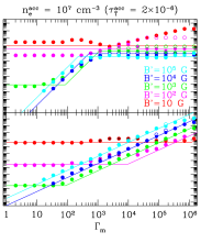
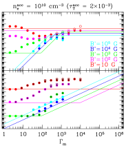
Figure 4: Synchrotron and inverse Compton peaks: comparison with analytical estimates. The photon peak energy of the synchrotron (bottom) and inverse Compton (top) components is plotted as a function of the initial minimum Lorentz factor of the accelerated electrons $\Gamma_{\mathrm{m}}$, for five different values of the magnetic field (color coded) and increasing values of the accelerated electron density $n_{\mathrm{e}}^{\mathrm{acc}}$ in the three panels. The dynamical timescale is fixed to $t^{\prime}_{\mathrm{ex}}=10\ \mathrm{s}$. Values obtained from our radiative code are indicated with open (resp. filled) circles corresponding to calculations without (resp. with) $\gamma\gamma$ annihilation. In the bottom panels, when the circle is filled with a black cross, the inverse Compton process is dominant compared to the synchrotron radiation. These results are compared to the analytical estimates (solid lines) discussed in the text: Eq. (34) for the synchrotron component and Eqs. (43) renormalized by a factor $10$, (45) renormalized by a factor $0.1$ and (LABEL:eq:emic) for the inverse Compton component. Note that, in the bottom panels, the transition between the horizontal and rising branches of the analytical estimate for $\epsilon_{\mathrm{p,syn}}$ corresponds to the transition between the synchrotron slow and fast cooling regimes.

Inverse Compton component.

If most scatterings between relativistic electrons and synchrotron photons occur in Thomson regime, the peak of the inverse Compton component is expected at $\epsilon_{\mathrm{ic,p}}\simeq\Gamma_{\mathrm{p}}^{2}\epsilon_{\mathrm{p,syn}}$, i.e.

$$h\nu^{\prime}_{\mathrm{p,ic}}\simeq 1.7\ \mathrm{keV}\ \left(\frac{B^{\prime}}{1000\ \mathrm{G}}\right)\left(\frac{\Gamma_{\mathrm{p}}}{100}\right)^{4}\ .$$ (43)

The Thomson approximation is valid as long as $\Gamma_{\mathrm{p}}\epsilon_{\mathrm{p,syn}}\ll 1$, i.e.

$$\Gamma_{\mathrm{p}}\ll\Gamma_{\mathrm{KN}}\simeq 3.0\times 10^{3}\ \left(\frac{B^{\prime}}{1000\ \mathrm{G}}\right)^{-1/3}\ ,$$ (44)

which corresponds to

$$h\nu^{\prime}_{\mathrm{p,ic}}\ll h\nu^{\prime}_{\mathrm{KN}}\simeq\Gamma_{\mathrm{KN}}m_{\mathrm{e}}c^{2}\simeq 1.3\ \mathrm{GeV}\ \left(\frac{B^{\prime}}{1000\ \mathrm{G}}\right)^{-1/3}\ .$$ (45)

A severe reduction of the high-energy spectrum should always be expected above $\nu^{\prime}_{\mathrm{KN}}$ in the comoving frame due to Klein-Nishina corrections to the inverse Compton cross-section. Even more, the maximum Lorentz factor of the relativistic electrons given by Eq. (9) leads to an absolute maximum energy $\sim\Gamma_{\mathrm{M}}m_{\mathrm{e}}c^{2}$ for a scattered photon, i.e.

$$h\nu^{\prime}_{\mathrm{M,ic}} \simeq \min{\left\{1.9\ \mathrm{TeV}\left(\frac{B^{\prime}}{1000\ \mathrm{G}}\right)^{-1/2}\!\!\!\!\!\!\!;\ 9000\ \mathrm{TeV}\left(\frac{B^{\prime}}{1000\ \mathrm{G}}\right)\left(\frac{t^{\prime}_{\mathrm{ex}}}{1\ \mathrm{s}}\right)\right\}}\ .$$

Again, except for very weak magnetic fields and very short dynamical timescales, the maximum inverse Compton frequency is always given by the first limit (acceleration limitation due to radiative losses). From these estimates, one can deduce that the peak of the inverse Compton component should be found in all cases at the frequency $\nu^{\prime}\simeq\min{\left\{\nu^{\prime}_{\mathrm{p,ic}};\ \nu^{\prime}_{\mathrm{KN}};\ \nu^{\prime}_{\mathrm{M,ic}}\right\}}$. Fig. 4 (top panels) show that numerical results of our radiative code are in a reasonable agreement with these theoretical predictions, as long as inverse Compton scatterings are not the dominant cooling process for electrons. The scaling in equation (43) appears to be correct but the normalization seems to be underestimated by a factor $\sim 10$. When Klein-Nishina corrections become important, the peak of the inverse Compton component appears typically at frequency $\sim 0.1\nu^{\prime}_{\mathrm{KN}}$ compared to Eq. (45). This is not surprising since the cross section for scatterings of a photon with frequency $\nu^{\prime}$ by an electron with Lorentz factor $\gamma$ shows non negligible Klein-Nishina deviations well below the limit $h\nu^{\prime}=\gamma m_{\mathrm{e}}c^{2}$. Significant deviations of one order of magnitude from the simple estimate $0.1\nu^{\prime}_{\mathrm{KN}}$ can be observed (see the cases with a weak magnetic field in Fig. 4).

When the Thomson regime is valid, the ratio of the inverse Compton over the synchrotron power is given by the Compton parameter, defined as the ratio of the energy density in photons over the magnetic energy density, $Y=u_{\mathrm{rad}}/\left(\left.B^{\prime}\right.^{2}/8\pi\right)$. This quantity is time-dependent. However, when not stated otherwise, $Y$ stands in this paper for the final value of the Compton parameter at $t^{\prime}_{\mathrm{ex}}$. As long as $Y<1$, synchrotron losses dominate, the seed photons for inverse Compton scatterings have the spectrum which is given above by Eqs. (30) and  (31), and the distribution of the electrons responsible for the scatterings is close to the broken-power law distribution $\bar{n}(\gamma)$ described by Sari et al. (1998). The corresponding spectral shape of the inverse Compton component has been derived by Sari & Esin (2001) and is given in their appendix A. It is based on the integration of the approximate relation

$$\left.n_{\nu^{\prime}}\right|_{\mathrm{ic}}\simeq t^{\prime}_{\mathrm{ex}}\int d\gamma\ \bar{n}(\gamma)\frac{\bar{P}^{\mathrm{\,ic}}_{\nu^{\prime}}(\gamma)}{h\nu^{\prime}}\ ,$$ (47)

where $\bar{n}(\gamma)$ is the time-averaged electron distribution predicted by Eq. (LABEL:eq:nbarge) and $\bar{P}^{\mathrm{\,ic}}_{\nu^{\prime}}(\gamma)$ is the inverse Compton power radiated at frequency $\nu^{\prime}$ by an electron with Lorentz factor $\gamma$, computed assuming a seed photon distribution equal to the standard, time-averaged, synchrotron spectrum given by Sari et al. (1998). Instead of the complete expression of $P^{\mathrm{ic}}_{\nu^{\prime}}(\gamma)$ (see appendix A), the authors use a simplified kernel (which is equivalent to assume Thomson regime everywhere) so that the integration can be made analytically. In the present study, both the electron and photon distributions are time-dependant, which leads to significant differences in the high-energy spectrum compared to the time-averaged approach. This will be further discussed later on.

The intensity of the inverse Compton component is

$$\left.\epsilon^{2}n_{\epsilon}\right|_{\mathrm{ic}}\simeq Y\left.\epsilon^{2}n_{\epsilon}\right|_{\mathrm{syn}}\ .$$ (48)

The Compton parameter in this case equals

$$Y \simeq \frac{4}{3}\frac{p-1}{p-2}\tau_{\mathrm{T}}^{\mathrm{acc}}\Gamma_{\mathrm{m}}\Gamma_{\mathrm{c}}\times\left\{\begin{array}[]{cl}1&\mathrm{if}\ \Gamma_{\mathrm{m}}>\Gamma_{\mathrm{c}}\ ,\\ \left(\frac{\Gamma_{\mathrm{m}}}{\Gamma_{\mathrm{c}}}\right)^{p-2}&\mathrm{if}\ \Gamma_{\mathrm{m}}<\Gamma_{\mathrm{c}}\ \mathrm{and}\ 2<p<3\ ,\\ {\Gamma_{\mathrm{m}}}/{\Gamma_{\mathrm{c}}}&\mathrm{if}\ \Gamma_{\mathrm{m}}<\Gamma_{\mathrm{c}}\ \mathrm{and}\ p>3\ .\\ \end{array}\right.$$ (52)

Note that the term $\frac{4}{3}\frac{p-1}{p-2}\tau_{\mathrm{T}}^{\mathrm{acc}}\Gamma_{\mathrm{m}}\Gamma_{\mathrm{c}}$ is simply equal to $u_{\mathrm{e}}^{\mathrm{acc}}/u_{\mathrm{B}}$, i.e. $\epsilon_{\mathrm{e}}/\epsilon_{\mathrm{B}}$ using the standard parameterization of the microphysics. In synchrotron fast cooling regime, the value of $Y$ can be understood as follows: due to a short synchrotron timescale, the region populated with relativistic electrons has a typical size $\sim c\,t^{\prime}_{\mathrm{syn}}\left(\Gamma_{\mathrm{m}}\right)$. The effective Thomson optical depth for relativistic electrons is $\sim\sigma_{\mathrm{T}}n_{\mathrm{e}}^{\mathrm{acc}}ct^{\prime}_{\mathrm{syn}}\left(\Gamma_{\mathrm{m}}\right)$. In Thomson regime, the frequency of a photon scattered by an electron with Lorentz factor $\gamma$ is multiplied by $\gamma^{2}$. Therefore, the Compton parameter $Y$ is approximatively given by

$$Y\simeq\frac{4}{3}\frac{p-1}{p-2}\left(\sigma_{\mathrm{T}}n_{\mathrm{e}}^{\mathrm{acc}}ct^{\prime}_{\mathrm{syn}}\left(\Gamma_{\mathrm{m}}\right)\right)\Gamma_{\mathrm{m}}^{2}\$$ (54)

which leads to the expression given above. On the other hand, in synchrotron slow cooling regime, the size of the region populated by relativistic electrons is now given by $\sim ct^{\prime}_{\mathrm{ex}}$ and therefore the Thomson optical depth for relativistic electron becomes much larger $\sim\sigma_{\mathrm{T}}n_{\mathrm{e}}^{\mathrm{acc}}ct^{\prime}_{\mathrm{ex}}$, which leads to Eq. (LABEL:eq:Y) for $p>3$. In the case where $2<p<3$, this equation is corrected by a factor $\left(\Gamma_{\mathrm{c}}/\Gamma_{\mathrm{m}}\right)^{3-p}>1$ as the typical Lorentz factor of scattering electrons is at an intermediate value between $\Gamma_{\mathrm{m}}$ and $\Gamma_{\mathrm{c}}$.

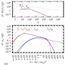
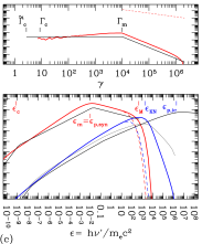
Figure 5: Synchrotron and Inverse Compton spectral components: comparison with analytical estimates. The time-averaged electron distribution and the final photon spectrum are shown for 3 different cases: (a) $\Gamma_{\mathrm{m}}=10^{2}$ and $n_{\mathrm{e}}^{\mathrm{acc}}=10^{8}\ \mathrm{cm^{-3}}$; (b) $\Gamma_{\mathrm{m}}=10^{2}$ and $n_{\mathrm{e}}^{\mathrm{acc}}=10^{10}\ \mathrm{cm^{-3}}$; (c) $\Gamma_{\mathrm{m}}=10^{4}$ and $n_{\mathrm{e}}^{\mathrm{acc}}=10^{8}\ \mathrm{cm^{-3}}$. In all cases, $p=2.5$, $B^{\prime}=3000\ \mathrm{G}$ and $t^{\prime}_{\mathrm{ex}}=10\ \mathrm{s}$. Synchrotron self-absorption and $\gamma\gamma$ annihilation are not included in the calculation. The time-averaged electron distribution obtained with our radiative code is plotted in the top panel with a red line and compared to the analytical prediction in black. The characteristic electron Lorentz factors discussed in the text are indicated with vertical bars. The initial distribution is also plotted with a dotted red line. The synchrotron (resp. inverse Compton) component of the final photon spectrum is plotted in the bottom panel with a red (resp. blue) line and is compared to the analytical estimate in black (thick line: analytical estimate by Sari & Esin (2001); thin line: semi-analytical estimate described in the text, which includes Klein-Nishina corrections). For indication, the result of the numerical calculation including $\gamma\gamma$ annihilation is also shown in dashed red and blue lines. The characteristic photon frequencies discussed in the text are indicated with vertical bars. Klein-Nishina corrections are negligible (except at high energy) in case (a) and (b). Synchrotron radiation is dominant in cases (a) and (c), whereas inverse Compton scatterings dominate in case (b).

As shown in case (a) of Fig. 5, except at very high energies (above $h\nu^{\prime}_{\mathrm{KN}}$), our numerical calculations are in very good agreement with the approximate spectrum given by Sari & Esin (2001), as long as $Y<1$. Above $\nu^{\prime}_{\mathrm{KN}}$, a better estimate is obtained when integrating numerically Eq. (47) with the same assumptions used by Sari & Esin (2001) (time-averaged electron and seed photon distributions) but using a complete kernel that includes Klein-Nishina corrections in the inverse Compton power (thin black line in Fig. 5). However, even using a more accurate cross section, Eq. (47) always overpredicts the inverse Compton emission at high energy. This systematic difference appears because the high energy photons in the inverse Compton component are due to the scatterings of photons at $\nu^{\prime}\sim\nu^{\prime}_{\mathrm{p,syn}}$ with high Lorentz factor electrons at $\gamma>\max{\left\{\Gamma_{\mathrm{m}};\Gamma_{\mathrm{c}}\right\}}$. In fast cooling regime, these two species are not present at the same time in the shocked region, as the duration necessary to form the synchrotron spectrum at $\nu^{\prime}_{\mathrm{p,syn}}$ is also the duration necessary to cool electrons above $\Gamma_{\mathrm{m}}$, i.e. the synchrotron timescale $t^{\prime}_{\mathrm{syn}}\left(\Gamma_{\mathrm{m}}\right)$. As Eq. (47) is based on a time-averaged approach, it cannot take into account such effects, related to the way the radiation field is built, and therefore it overestimates the spectrum above $\nu^{\prime}_{\mathrm{p,ic}}$. We checked that in synchrotron slow cooling regime the agreement is better above $\nu^{\prime}_{\mathrm{p,ic}}$ than what is observed in Fig. 5, but Eq. (47) is still overestimating the high-energy component when evaluating the scatterings by fast cooling electrons (i.e. electrons with $\gamma>\Gamma_{\mathrm{c}}$).

When $Y>1$, inverse Compton losses become dominant. Then, the effective radiative timescale is shorter than the synchrotron timescale (by a factor $\sim(1+Y)$), the effective critical Lorentz factor is reduced ($\tilde{\Gamma}_{\mathrm{c}}\sim\Gamma_{\mathrm{c}}/(1+Y)$) and the corresponding frequency $\epsilon_{\mathrm{c}}$ in the synchrotron spectrum (Eqs. (30) and (31)) as well. The intensity of the synchrotron component is reduced by a factor $1/(1+Y)$. These corrections are however very approximate and valid only in Thomson regime. Our tests show that when inverse Compton scatterings become dominant, the modified cooling rate of electrons affects the time-averaged distribution $\bar{n}(\gamma)$ (which differs from the standard broken-law distribution given by Eq. (LABEL:eq:nbarge)), and therefore the distribution of seed synchrotron photons becomes different from the standard synchrotron spectrum given by Eqs. (30) and (31). This is well seen in cases (b) and (c) in Fig. 5. In fact, in this case, the approach used by Sari & Esin (2001) is not appropriate because the spectrum of the seed photons cannot be predicted by an a priori calculation including the synchrotron process only: the resulting spectrum has not enough time to be built when inverse Compton losses are included. This effect becomes stronger when Klein-Nishina corrections are important, as the ratio of the inverse Compton to the synchrotron power becomes highly dependant on the electron Lorentz factor. As seen in Fig. 5, the low-energy slope of the synchrotron spectrum is steeper in that case. Such a behavior is in agreement with the theoretical predictions made by Derishev et al. (2001). We plan to investigate in a forthcoming paper if this could reconcile the synchrotron radiation with the observed distribution of the low-energy photon index in BATSE bursts (Preece et al. 2000), which differs from the simplest prediction of the fast cooling synchrotron spectrum (Ghisellini et al. 2000) as its mean value is close to $\alpha\sim-1$.

Formation of the radiation field.

These results show that the high energy component of the photon spectrum cannot be estimated accurately without understanding how the radiation field (seed photons for inverse Compton scatterings) is formed. Initially, no photons are present and synchrotron radiation is always dominant ($Y(t^{\prime}=0)=0$). The Compton parameter is an increasing function of time, due to the progressive building of the radiation field (see Fig. 20). When synchrotron radiation is the dominant process, the radiation field increases up to $t^{\prime}\sim t^{\prime}_{\mathrm{syn}}\left(\Gamma_{\mathrm{m}}\right)=t^{\prime}_{\mathrm{ex}}{\Gamma_{\mathrm{c}}}/{\Gamma_{\mathrm{m}}}$ in fast cooling regime, and then it saturates. In slow cooling regime, it increases up to $t^{\prime}\simeq t^{\prime}_{\mathrm{ex}}$. In both cases, the time evolution of the Compton parameter, $Y(t^{\prime})$, can be evaluated analytically (as shown in appendix C) and its asymptotic value $Y_{\mathrm{ex}}=Y\left(t^{\prime}_{\mathrm{ex}}\right)$ is given by Eq. (LABEL:eq:Y), as long as most scatterings occur in Thomson regime. In fast cooling regime, a necessary condition to have a dominant inverse Compton component in the final spectrum is therefore $u_{\mathrm{e}}^{\mathrm{acc}}/u_{\mathrm{B}}=\epsilon_{\mathrm{e}}/\epsilon_{\mathrm{B}}>1$. It is however not a sufficient condition, as the intensity of the inverse Compton component can be attenuated by Klein-Nishina effects, and also by $\gamma\gamma$ annihilation.

When $Y_{\mathrm{ex}}>1$, the impact of inverse Compton scatterings on the electron distribution will depend on the time $t^{\prime}_{\mathrm{ic}}$ where $Y(t^{\prime}_{\mathrm{ic}})\sim 1$, i.e. the time when inverse Compton scatterings become the dominant process of cooling. Indeed, only the distribution of electrons below $\Gamma_{\mathrm{c}}(t^{\prime}_{\mathrm{ic}})$ can be affected by the new dominant cooling process, as electrons at higher Lorentz factor have already cooled by synchrotron radiation. Here, the Lorentz factor $\Gamma_{\mathrm{c}}(t^{\prime})$ is defined as the Lorentz factor giving a synchrotron timescale of the order of $t^{\prime}$, i.e. $t^{\prime}_{\mathrm{syn}}\left(\Gamma_{\mathrm{c}}(t^{\prime})\right)\simeq t^{\prime}$. With this definition $\Gamma_{\mathrm{c}}=\Gamma_{\mathrm{c}}(t^{\prime}_{\mathrm{ex}})$. In the synchrotron fast cooling case, the synchrotron spectrum around the peak at $\nu^{\prime}_{\mathrm{m}}$ will be affected by inverse Compton scatterings if this process becomes dominant at very early times, i.e if $\Gamma_{\mathrm{c}}(t^{\prime}_{\mathrm{ic}})>\Gamma_{\mathrm{m}}$, which is equivalent to $t^{\prime}_{\mathrm{ic}}<t^{\prime}_{\mathrm{syn}}\left(\Gamma_{\mathrm{m}}\right)=t^{\prime}_{\mathrm{ex}}\Gamma_{\mathrm{c}}/\Gamma_{\mathrm{m}}$.

When inverse Compton scatterings are extremely efficient, they can represent the dominant electron cooling process, even at early times. When this happens, the maximum Lorentz factor of accelerated electrons $\Gamma_{\mathrm{M}}$ is overestimated in Eq. (9). From the evolution of $Y(t^{\prime})$ discussed in appendix C, one can deduce the value reached by the Compton parameter when electrons at $\Gamma_{\mathrm{M}}$ have cooled, i.e.

$$Y_{\mathrm{M}} = Y\left(t^{\prime}_{\mathrm{syn}}\left(\Gamma_{\mathrm{M}}\right)\right)\simeq\frac{4}{3}\frac{p-1}{3-p}\tau_{\mathrm{T}}^{\mathrm{acc}}\Gamma_{\mathrm{c}}\Gamma_{\mathrm{m}}\left(\frac{\Gamma_{\mathrm{m}}}{\Gamma_{\mathrm{M}}}\right)^{p-2}\left[1-\left(\frac{\Gamma_{\mathrm{m}}}{\Gamma_{\mathrm{M}}}\right)^{3-p}\right]\ .$$

Here it is assumed that $t^{\prime}_{\mathrm{syn}}\left(\Gamma_{\mathrm{M}}\right)\ll t^{\prime}_{\mathrm{ex}}$ in Eq. (80), which is always the case when the radiative cooling is the dominant limiting process for electron acceleration. If $Y_{\mathrm{M}}<1$, the estimate of the electron maximum Lorentz factor $\Gamma_{\mathrm{M}}$ given by Eq. (9) is valid as the radiative timescale of electrons at $\Gamma_{\mathrm{M}}$ is accurately given by their synchrotron timescale. On the other hand, if $Y_{\mathrm{M}}>1$, it is possible that the value of $\Gamma_{\mathrm{M}}$ given by Eq. (9) is overestimated. It is not always the case as the value of $Y_{\mathrm{M}}$ is computed assuming inverse Compton scatterings in Thomson regime. The true value of $Y_{\mathrm{M}}$ can therefore be reduced by Klein-Nishina corrections. In practice, we checked that our assumptions regarding the maximum Lorentz factor of electrons are consistent in all the cases presented in this paper.

Photon–photon annihilation.

The timescale associated with $\gamma\gamma$ annihilation is given by

$$t^{\prime}_{\mathrm{\gamma\gamma}}(\nu^{\prime})\simeq\left(\int d\tilde{\nu}^{\prime}\ n_{\tilde{\nu}^{\prime}}c\sigma_{\gamma\gamma}(\nu^{\prime},\tilde{\nu}^{\prime})\right)^{-1}\!\!\!\simeq\left.\frac{5h}{c\sigma_{\mathrm{T}}}\frac{1}{\left(h\tilde{\nu}^{\prime}n_{\tilde{\nu}^{\prime}}\right)}\right|_{\tilde{\nu}^{\prime}=\frac{\left(m_{\mathrm{e}}c^{2}\right)^{2}}{h^{2}\nu^{\prime}}}\ ,$$ (56)

where a Dirac approximation has been used for the cross section (Gould & Schréder 1967). The cutoff will occur at high energy and the corresponding photons will annihilate with low-energy photons whose distribution is approximatively given by the synchrotron spectrum described in Eqs. (30) and (31). An approximate shape of the absorbed spectrum can then be computed by attenuating the emitted spectrum by a factor

$$e^{-\tau_{\gamma\gamma}(\nu^{\prime})}=\frac{t^{\prime}_{\mathrm{\gamma\gamma}}(\nu^{\prime})}{t^{\prime}_{\mathrm{ex}}}\left(1-e^{-t^{\prime}_{\mathrm{ex}}/t^{\prime}_{\mathrm{\gamma\gamma}}(\nu^{\prime})}\right)\ ,$$ (57)

where $\tau_{\gamma\gamma}(\nu^{\prime})$ is the $\gamma\gamma$ annihilation optical depth at frequency $\nu^{\prime}$. A comparison with the results of the detailed radiative code shows that this approximate treatment is again accurate as long as inverse Compton losses are not the dominant cooling process for electrons, i.e. as long as the low-energy photon distribution is well described by the standard synchrotron spectrum. In Fig. 5, the attenuation of the spectrum at high energy due to $\gamma\gamma$ annihilation is shown in different cases with an increasing importance of inverse Compton scatterings.

3.3 The shape of the radiated spectrum

We define a “reference case” corresponding to the physical conditions in the shocked material of the example in Fig. 1 at $t=1.9\times 10^{4}\ \mathrm{s}$, i.e. $\Gamma_{*}\simeq 240$, $\rho_{*}\simeq 6.8\times 10^{-15}\ \mathrm{g\leavevmode\nobreak\ cm^{-3}}$, $\epsilon_{*}/c^{2}\simeq 8.0\times 10^{-2}$ and $t^{\prime}_{\mathrm{ex}}=80\ \mathrm{s}$. For $\epsilon_{\mathrm{e}}=\epsilon_{\mathrm{B}}=1/3$, $p=2.5$ and $\zeta=10^{-2}$ (only 1 % of the electrons are accelerated), this leads to $B^{\prime}\simeq 2000\ \mathrm{G}$, $n_{\mathrm{e}}^{\mathrm{acc}}\simeq 4.1\times 10^{7}\ \mathrm{cm^{-3}}$ and $\Gamma_{\mathrm{m}}=1.6\times 10^{3}$. This choice of parameters is motivated by the study presented in Daigne & Mochkovitch (1998) which favors the case where the magnetic field is high and where only a small fraction of electrons is accelerated, as these two conditions are required for the synchrotron peak to be in the BATSE range. Starting from this “reference case”, one of the parameters $\left(\Gamma_{\mathrm{m}},B^{\prime},t^{\prime}_{\mathrm{ex}},n^{\mathrm{acc}}_{\mathrm{e}}\right)$ is varied, while all other parameters are maintained constant. The resulting evolution of the spectrum is plotted in Fig. 6.

Effect of the initial minimum Lorentz factor of relativistic electrons.

Panel (a) shows the effect of $\Gamma_{\mathrm{m}}$. The spectrum is the combination of a low-energy component due to the synchrotron emission in fast cooling regime, and a high-energy component due to inverse Compton emission, partially suppressed due to $\gamma\gamma$ annihilation. (i) Synchrotron emission. The evolution of the low-energy peak (synchrotron emission) with $\Gamma_{\mathrm{m}}$ follows exactly the prediction of the analytical estimate in fast cooling regime: the spectrum peaks at the frequency $\nu^{\prime}_{\mathrm{m}}$ (synchrotron frequency of electrons with $\gamma=\Gamma_{\mathrm{m}}$) that scales as $\nu^{\prime}_{\mathrm{m}}\propto\Gamma_{\mathrm{m}}^{2}$ and the corresponding peak intensity follows $\left(\left.\nu^{\prime}\right.^{2}n_{\nu^{\prime}}\right)_{\nu^{\prime}=\nu^{\prime}_{\mathrm{m}}}\propto\Gamma_{\mathrm{m}}$ (Sari et al. 1998). A dashed line of slope $1/2$ in the $\log{\nu^{\prime}}$–$\log{\left(\left.\nu^{\prime}\right.^{2}n_{\nu^{\prime}}\right)}$ diagram indicates the predicted position of the synchrotron peak. The agreement with the numerical calculation is excellent; (ii) inverse Compton scattering. For low $\Gamma_{\mathrm{m}}$, as synchrotron photons peak at low energy, inverse Compton scatterings occur in Thomson regime. Then, from Eq. (LABEL:eq:Y), the Compton parameter $Y$ scales as $Y\propto\Gamma_{\mathrm{m}}$. This is indeed shown in panel (a), where the intensity of the inverse Compton component increases when $\Gamma_{\mathrm{m}}$ increases. The high-energy peak due to inverse Compton emission follows exactly the predicted line of slope $1/2$ in the $\log{\nu^{\prime}}$–$\log{\left(\left.\nu^{\prime}\right.^{2}n_{\nu^{\prime}}\right)}$ diagram (the peak energy scales as $\Gamma_{\mathrm{m}}^{2}\nu_{\mathrm{m}}\propto\Gamma_{\mathrm{m}}^{4}$ and the intensity scales as $Y\left(\left.\nu^{\prime}\right.^{2}n_{\nu^{\prime}}\right)_{\mathrm{m}}\propto\Gamma_{\mathrm{m}}^{2}$). As $\Gamma_{\mathrm{m}}$ increases, the synchrotron emission peaks at higher energy and more and more photons have energies comparable with $m_{\mathrm{e}}c^{2}$ in the frame of electrons at $\gamma=\Gamma_{\mathrm{m}}$. Therefore the efficiency of inverse Compton emission is strongly reduced by Klein-Nishina corrections; (iii) $\gamma\gamma$ annihilation. this process becomes more efficient for high $\Gamma_{\mathrm{m}}$ as the synchrotron emission peaks at higher energy and more photons are above the threshold. In conclusion, these two effects combine so that the high-energy component is most intense for intermediate values of $\Gamma_{\mathrm{m}}$.

Minimum electron Lorentz factor	Magnetic field
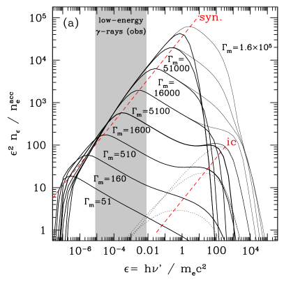
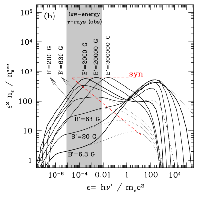
Adiabatic cooling timescale	Density of accelerated electrons

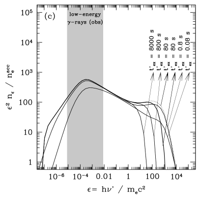
Figure 6: Emitted spectrum in the comoving frame. We consider a “reference case” defined by $\Gamma_{\mathrm{m}}=1600$, $B^{\prime}=2000\ \mathrm{G}$, $t^{\prime}_{\mathrm{ex}}=80\ \mathrm{s}$ and $n_{\mathrm{e}}^{\mathrm{acc}}=4.1\times 10^{7}\ \mathrm{cm^{-3}}$ corresponding to the physical conditions in the shocked material at $t=1.9\times 10^{4}\ \mathrm{s}$ in the example shown in Fig. 1, for $\epsilon_{\mathrm{e}}=\epsilon_{\mathrm{B}}=1/3$, $p=2.5$ and $\zeta=10^{-2}$ (see text). Each panel shows the evolution of the spectrum when one parameter is varied, while all other parameters are maintained constant: (a) effect of the initial minimum Lorentz factor of the electrons $\Gamma_{\mathrm{m}}$. For low $\Gamma_{\mathrm{m}}$, the weak inverse Compton component is shown with a dotted line. The high-energy component that would be obtained without $\gamma\gamma$ annihilation is plotted with a thin solid line. Two dashed lines indicate the predicted position of the synchrotron peak in fast cooling regime, and of the inverse Compton peak in Thomson regime; (b) effect of the magnetic field $B^{\prime}$. For low $B^{\prime}$, the weak synchrotron component is plotted with a dotted line. The high-energy component that would be obtained without $\gamma\gamma$ annihilation is plotted with a dotted line for $B^{\prime}=6.3\ \mathrm{G}$ and $B^{\prime}=2000\ \mathrm{G}$. The dashed line indicates the predicted position of the synchrotron peak in slow and fast cooling regime. ; (c) effect of the adiabatic cooling timescale $t^{\prime}_{\mathrm{ex}}$. For $t^{\prime}_{\mathrm{ex}}=80\ \mathrm{s}$, the spectrum that would be obtained without $\gamma\gamma$ annihilation is plotted with a dotted line; (d) effect of the initial density of relativistic electrons $n_{\mathrm{e}}^{\mathrm{acc}}$. For high $n_{\mathrm{e}}^{\mathrm{acc}}$, the spectrum that would be obtained without $\gamma\gamma$ annihilation is plotted with a dotted line. In all panels, the approximate range of low-energy gamma-rays (1 keV-1 MeV) is indicated by the gray area, assuming $z=1$ and $\Gamma_{*}=240$.

Effect of the magnetic field.

Panel (b) shows the effect of $B^{\prime}$. This effect is more complicated than for $\Gamma_{\mathrm{m}}$, especially at low energy. (i) Synchrotron emission. For very weak magnetic fields, inverse Compton scatterings are so efficient that the effective electron radiative timescale is short compared to the adiabatic cooling time and most of their energy is radiated. This high radiative efficiency is reached despite the fact that synchrotron radiation occurs in slow cooling regime ($t^{\prime}_{\mathrm{syn}}\left(\Gamma_{\mathrm{m}}\right)>t^{\prime}_{\mathrm{ex}}$). In other terms, this situation corresponds to the following ordering of characteristic electron Lorentz factors: $\tilde{\Gamma}_{\mathrm{c}}<\Gamma_{\mathrm{m}}<\Gamma_{\mathrm{c}}$. For more intense magnetic fields, the electron synchrotron timescale is reduced and synchrotron radiation operates in fast cooling regime ($\tilde{\Gamma}_{\mathrm{c}}<\Gamma_{\mathrm{c}}<\Gamma_{\mathrm{m}}$). The complex evolution of the synchrotron peak with $B^{\prime}$ observed in panel (b) is then due to the transition between synchrotron slow (low $B^{\prime}$) and fast (high $B^{\prime}$) cooling regime. For low $B^{\prime}$, the synchrotron peak is given by the synchrotron frequency $\nu^{\prime}_{\mathrm{c}}$ of electrons with $\gamma=\Gamma_{\mathrm{c}}$ and decreases with $B^{\prime}$ as $\nu^{\prime}_{\mathrm{c}}\propto\left.B^{\prime}\right.^{-3}$. The corresponding peak intensity follows $\left(\left.\nu^{\prime}\right.^{2}n_{\nu^{\prime}}\right)_{\nu^{\prime}=\nu^{\prime}_{\mathrm{c}}}\propto B^{2\left(p-2\right)}$ (Sari et al. 1998), so that the low-energy peak follows a line of slope $-2(p-2)/3$ in the $\log{\nu^{\prime}}$–$\log{\left(\left.\nu^{\prime}\right.^{2}n_{\nu^{\prime}}\right)}$ diagram. For larger values of $B^{\prime}$, synchrotron radiation is in fast cooling regime and the peak is given by $\nu^{\prime}_{\mathrm{m}}$, which scales as $\nu^{\prime}_{\mathrm{m}}\propto B^{\prime}$. The corresponding peak intensity does not vary with $B^{\prime}$ and therefore the low-energy peak falls into an horizontal line for high magnetic fields in the same diagram; (ii) inverse Compton scattering. For low magnetic fields, when the synchrotron radiation is in slow cooling regime, the typical size of the region populated by relativistic electrons is $\sim ct^{\prime}_{\mathrm{ex}}$, that is much larger than in the synchrotron fast cooling regime. Therefore, even in Klein-Nishina regime, inverse Compton scatterings are extremely efficient due to the increased optical depth. As $B^{\prime}$ increases, the synchrotron peak energy decreases and inverse Compton scatterings can occur in the Thomson regime. However, as soon as the magnetic field is high enough so that the synchrotron radiation enters the fast cooling regime, the Thomson optical depth for relativistic electrons is reduced as the size of the region populated with relativistic electrons is $\sim ct^{\prime}_{\mathrm{syn}}\left(\Gamma_{\mathrm{m}}\right)\ll ct^{\prime}_{\mathrm{ex}}$. In addition, the synchrotron peak energy increases, so that Klein-Nishina corrections are present. These two effects result in a strong decrease of the inverse Compton efficiency; (iii) $\gamma\gamma$ annihilation. This process becomes important for a low magnetic field $B^{\prime}$, when the emission at high energy is most efficient. In conclusion, weak magnetic fields favor a strong high-energy emission, even when $\gamma\gamma$ annihilation is non negligible.

Effect of the adiabatic cooling timescale.

The effect of $t^{\prime}_{\mathrm{ex}}$ is shown in panel (c). For a magnetic field $B^{\prime}=2000\ \mathrm{G}$ and an initial minimum electron Lorentz factor $\Gamma_{\mathrm{m}}=1600$ as in our reference case, the synchrotron timescale equals $t^{\prime}_{\mathrm{syn}}\left(\Gamma_{\mathrm{m}}\right)\simeq 0.12\ \mathrm{s}$. (i) for high values, $t^{\prime}_{\mathrm{ex}}\gg 0.1\ \mathrm{s}$, the spectrum at low energy does not depend on $t^{\prime}_{\mathrm{ex}}$ as it is produced by synchrotron radiation in fast cooling regime. Inverse Compton scatterings are rare because relativistic electrons are present only in a small fraction of the volume of the shocked region ($\sim t^{\prime}_{\mathrm{syn}}/t^{\prime}_{\mathrm{ex}}$, see above). On the other hand the absorption due to $\gamma\gamma$ annihilation increases with $t^{\prime}_{\mathrm{ex}}$ because the effective size of the region populated with photons is larger and the probability to have photon-photon interactions is increased; (ii) for low values, $t^{\prime}_{\mathrm{ex}}\ll 0.1\ \mathrm{s}$, the radiative efficiency decreases strongly as electrons are in slow cooling regime; (iii) for intermediate values such as $t^{\prime}_{\mathrm{ex}}\ga t^{\prime}_{\mathrm{syn}}\left(\Gamma_{\mathrm{m}}\right)$, relativistic electrons can radiate efficiently and still populate most of the shocked region. This favors a brighter high energy component as inverse Compton scatterings are more frequent. In conclusion, an intense high energy component in the photon spectrum is favored by intermediate values of the adiabatic cooling timescale.

Effect of the initial density of relativistic electrons.

The effect of $n_{\mathrm{e}}^{\mathrm{acc}}$ is shown in panel (d). At low densities, the optical depth for inverse Compton scatterings is low, so the spectrum is simply a synchrotron spectrum in fast cooling regime. At high densities the intensity of the inverse Compton component increases, as well as the absorption due to $\gamma\gamma$ annihilation, because the number of available high-energy photons scales with the density of emitting electrons. Therefore the most intense high-energy component is again obtained for intermediate values of the relativistic electron density, when inverse Compton scatterings are efficient and the attenuation due to $\gamma\gamma$ annihilation is still not too strong.

This parameter study aims at identifying the physical conditions in the comoving frame leading to an intense high energy emission. Fig. 7 shows the distributions of the parameters corresponding to cases with an efficient inverse Compton emission (more than 50 % of the radiated energy is due to inverse Compton scatterings) and a limited $\gamma\gamma$ annihilation (negligible attenuation at the peak of the inverse Compton component). The most intense high-energy components are obtained for low values of the magnetic field ($B^{\prime}\la 100\ \mathrm{G}$) and for intermediate values of the electron minimum Lorentz factor ($\Gamma_{\mathrm{m}}\simeq 100-1000$), of the adiabatic time scale ($t^{\prime}_{\mathrm{ex}}\simeq 3-30\ \mathrm{s}$) and of the density $n_{\mathrm{e}}^{\mathrm{acc}}$ ($n_{\mathrm{e}}^{\mathrm{acc}}\simeq 10^{8}-10^{9}\ \mathrm{cm^{-3}}$).

Figure 7: Physical conditions in the shocked region (comoving frame) that favor an intense high energy component. From our exploration of the parameter study of the internal shock model (see Sect. 3) the histograms of the electron minimum Lorentz factor $\Gamma_{\mathrm{m}}$, the magnetic field $B^{\prime}$, the adiabatic cooling timescale $t^{\prime}_{\mathrm{ex}}$ and the initial density of accelerated electrons $n_{\mathrm{e}}^{\mathrm{acc}}$ are plotted for all models that satisfy the radiative efficiency and transparency conditions (see text). The shaded histograms show the models that fulfill the same conditions and, in addition, have an efficient inverse Compton emission (most of 50% of the electron energy which is radiated is due to inverse Compton scatterings) and a negligible $\gamma\gamma$ annihilation (defined as cases where the peak in $\nu F_{\nu}$ of the high-energy component is shifted by less than 10 % when including $\gamma\gamma$ annihilation).

4 Probing the parameter space of internal shocks

In the internal shock model, the four quantities studied in Sect. 3 are not independent. As described in Sect. 2, they are determined from two sets of parameters: the first set defines the dynamical evolution. In the simple two shell version of the model, these parameters are $\bar{\Gamma}$, $\kappa$, $\dot{E}$ and $\tau$. The second set is related to the unknown microphysics in the shocked region : $\epsilon_{\mathrm{B}}$, $\epsilon_{\mathrm{e}}$, $\zeta$ and $p$. Therefore, we have computed 7200 spectra corresponding to : (i) 4 values for the mean Lorentz factor in the outflow, $\log{\bar{\Gamma}}=1.5$, $2$, $2.5$ and $3$; (ii) 4 values for the contrast which characterizes the amplitude of the variations in the initial distribution of the Lorentz factor in the outflow, $\kappa=2.5$, $5$, $7.5$ and $10$; (iii) 6 values of the injected kinetic power during the relativistic ejection, $\log{\left(\dot{E}/1\ \mathrm{erg\leavevmode\nobreak\ s^{-1}}\right)}=50$, $51$, $52$, $53$, $54$ and $55$; (iv) 5 values for the variability timescale, $\log{\left(\tau/1\ \mathrm{s}\right)}=-2$, $-1$, $0$, $1$ and $2$; (v) 3 values for the fraction of the dissipated energy which is injected in the magnetic field, $\log{\epsilon_{\mathrm{B}}}=-3.5$, $-2$ and $-0.5$; (vi) 5 values for the fraction of electrons that are accelerated, $\log{\zeta}=-4$, $-3$, $-2$, $-1$ and $0$.

The moderate efficiency of the conversion of kinetic energy into internal energy by internal shocks imposes that a large fraction $\epsilon_{\mathrm{e}}$ of this dissipated energy is injected in relativistic electrons to maintain a reasonable total efficiency. Therefore we fix $\epsilon_{\mathrm{e}}=1/3$. In the example presented in Fig. 1, about $7\ \%$ of the kinetic energy is converted in internal energy by shock waves. If electrons are radiating efficiently, about $2\ \%$ of the initial kinetic energy will be radiated.

We also assume a slope $p=2.5$ for the electron distribution, except where mentioned otherwise. This new set of spectra will allow us to identify which properties of the outflow determine the shape of the high energy spectrum, and therefore help to identify physical diagnostics for future Fermi data.

Bulk Lorentz factor	Contrast
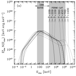
Injected kinetic power	Variability timescale
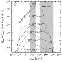
Fraction of energy injected in the magn. field	Fraction of accelerated electrons

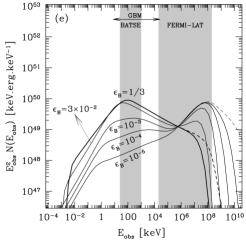
Figure 8: The effect of internal shock parameters on the emitted spectrum (“synchrotron case”). We use the simple two shell version of the internal shock model (see text) and define a “reference case” by $\bar{\Gamma}=300$, $\kappa=4$, $\dot{E}=10^{52}\ \mathrm{erg\leavevmode\nobreak\ s^{-1}}$, $\tau=1\ \mathrm{s}$, $\epsilon_{\mathrm{e}}=\epsilon_{\mathrm{B}}=1/3$, $\zeta=10^{-2}$ and $p=2.5$. Each panel shows the evolution of the observed spectrum (assuming $z=1$) when one parameter is varied, while all other parameters are maintained constant. Two effects can limit the parameter range: electrons become radiatively inefficient (“efficiency limit”) or the medium becomes optically thick due to the intense production of pairs (“transparency limit”). For each limiting case corresponding to the transparency limit (panels a,b,c,d), the spectrum that would be observed without $\gamma\gamma$ annihilation is plotted with a dashed line. (a) effect of $\bar{\Gamma}$. The transparency limit is reached for $\bar{\Gamma}<109$ and the efficiency limit for $\bar{\Gamma}>1400$ ; (b) effect of $\kappa$. The efficiency limit is reached for $\kappa<1.5$ and the transparency limit for $\kappa>12.5$; (c) effect of $\dot{E}$. The transparency limit is reached for $\dot{E}>2\times 10^{54}\ \mathrm{erg\leavevmode\nobreak\ s^{-1}}$; (d) effect of $\tau$. The transparency limit is reached for $\tau<0.008\ \mathrm{s}$; (e) effect of $\epsilon_{\mathrm{B}}$. The transparency limit is never reached. The spectrum that would be observed without $\gamma\gamma$ annihilation is plotted with a dashed line for $\epsilon_{\mathrm{B}}=10^{-5}$ and $\epsilon_{\mathrm{B}}=1/3$; (f) effect of $\zeta$. The transparency limit is never reached. The spectrum that would be observed without $\gamma\gamma$ annihilation is plotted with a dashed line for $\zeta=10^{-2}$.

4.1 The spectral shape of internal shock emission

The effect of the six parameters $\left(\bar{\Gamma},\kappa,\dot{E},\tau,\epsilon_{\mathrm{B}},\zeta\right)$ on the emitted spectrum is now studied. We define again a “reference case” by $\bar{\Gamma}=300$, $\kappa=4$, $\dot{E}=10^{52}\ \mathrm{erg\leavevmode\nobreak\ s^{-1}}$, $\tau=1\ \mathrm{s}$, $\epsilon_{\mathrm{B}}=1/3$ and $\zeta=10^{-2}$. Such a set of parameters corresponds to a “typical” GRB pulse with a peak energy $E_{\mathrm{p}}\simeq 200\ \mathrm{keV}$ (source frame) due to the synchrotron radiation. Fig. 8 shows the evolution of the observed spectrum when one of the parameters is varied, while all other parameters are maintained constant (assuming a redshift $z=1$).

Maximum radius to maintain a high radiative efficiency.

At very large distances from the source, the density becomes very low as well as the magnetic field. This increases the synchrotron timescale. In an equivalent way $\Gamma_{\mathrm{c}}$ is increasing and, at some maximum radius, can become of the order of $\Gamma_{\mathrm{m}}$ which strongly reduces the radiative efficiency. For such high radii, inverse Compton scatterings are rare due to a low density. This limit can then be evaluated by taking into account synchrotron radiation only. From Eqs. (1), (3), (6) and (18) the condition $\Gamma_{\mathrm{m}}>\Gamma_{\mathrm{c}}$ leads to

$$\left(\frac{(p-2)/(p-1)}{1/3}\right)\left(\frac{\epsilon_{\mathrm{B}}}{1/3}\right)\left(\frac{\epsilon_{\mathrm{e}}}{1/3}\right)\left(\frac{\zeta}{10^{-2}}\right)^{-1}$$

$$\times\left(\frac{f(\kappa)}{f(4)}\right)\left(\frac{\dot{E}}{10^{52}\ \mathrm{erg/s}}\right)\left(\frac{\bar{\Gamma}}{300}\right)^{-5}\left(\frac{\tau}{1\ \mathrm{s}}\right)^{-1} \ga 1.0\times 10^{-3}\ ,$$ (58)

with $f(\kappa)=(\kappa+1)^{6}(\kappa-1)(\sqrt{\kappa}-1)^{2}/\kappa^{9/2}$. For our reference case, when varying one parameter only, this condition leads to a maximum bulk Lorentz factor $\bar{\Gamma}\la 1200$, a minimum contrast $\kappa\ga 1.2$, a minimum injected kinetic power $\dot{E}\ga 1.0\times 10^{49}\ \mathrm{erg/s}$, a maximum timescale $\tau\la 1000\ \mathrm{s}$ and a minimum fraction of the energy injected into the magnetic field $\epsilon_{\mathrm{B}}\ga 3\times 10^{-4}$. The numerical results shown in Fig. 8 agree well with these analytical estimates.

Note that an additional condition should apply to limit the maximum radius of internal shocks (see e.g. Daigne & Mochkovitch 2007): most collisions should occur before the deceleration radius, otherwise the propagation of the reverse shock in the relativistic outflow will suppress the internal shock phase. For reasonable estimates of the external density, the deceleration radius is of the order of $10^{16}-10^{17}\ \mathrm{cm}$. From Eq. (1), this leads to a new constraint

$$\left(\frac{g(\kappa)}{g(4)}\right)\left(\frac{\bar{\Gamma}}{300}\right)^{2}\left(\frac{\tau}{1\ \mathrm{s}}\right)\la 110\left(\frac{R_{\mathrm{dec}}}{10^{17}\ \mathrm{cm}}\right)\ ,$$ (59)

with $g(\kappa)=\kappa^{2}/\left((\kappa-1)(\kappa+1)^{3}\right)$.

Maximum density to have an optically thin medium.

On the other end, if internal shocks occur close to the central source, the density will be high. The Thomson optical depth due to the ambient electrons and the pairs produced by $\gamma\gamma$ annihilation can then make the outflow optically thick. For our reference model, when varying one parameter only, $\tau_{\mathrm{T}}^{\mathrm{tot}}<1$ leads to a minimum value of $\bar{\Gamma}\ga 110$, a maximum value of $\kappa\la 13$, a maximum value of $\dot{E}\la 2\times 10^{54}\ \mathrm{erg\leavevmode\nobreak\ s^{-1}}$ and a minimum value of $\tau\ga 0.008\ \mathrm{s}$.

The synchrotron component at low energy.

As the scaling given by Eq. (34) for the synchrotron peak energy is quite accurate, it is not surprising to find that in most cases, the position of the synchrotron peak is simply given by (Barraud et al. 2005)

$$E_{\mathrm{syn,obs}}\propto\Gamma_{*}B^{\prime}\Gamma_{\mathrm{m}}^{2}\propto\Gamma_{*}\frac{\epsilon_{\mathrm{B}}^{1/2}\epsilon_{\mathrm{e}}^{2}}{\zeta^{2}}\rho_{\mathrm{*}}^{1/2}\epsilon_{\mathrm{*}}^{5/2}\propto\frac{\epsilon_{\mathrm{B}}^{1/2}\epsilon_{\mathrm{e}}^{2}}{\zeta^{2}}\Phi\left(\kappa\right)\frac{\dot{E}^{1/2}}{\bar{\Gamma}^{2}\tau}$$ (60)

with

$$\Phi(\kappa)=\frac{\left(\sqrt{\kappa}-1\right)^{5}\left(\kappa-1\right)\left(\kappa+1\right)^{3}}{\kappa^{7}}\ .$$ (61)

As predicted, the observed photon energy of the synchrotron peak increases (see Fig. 8) when (i) the Lorentz factor $\bar{\Gamma}$ decreases; (ii) the contrast $\kappa$ increases; (iii) the injected kinetic power $\dot{E}$ increases; (iv) the duration of the ejection $\tau$ decreases; (v) the fraction $\epsilon_{\mathrm{B}}$ increases; (vi) the fraction $\zeta$ decreases. This confirms that a low fraction of accelerated electrons is necessary to have a synchrotron peak in the gamma-ray range (Daigne & Mochkovitch 1998) and that X-ray flashes and X-ray rich gamma-ray bursts can be produced by internal shocks within “clean fireballs”, i.e. outflows having a high Lorentz factor $\bar{\Gamma}$ (small baryonic pollution) and a small contrast $\kappa$ (Barraud et al. 2005).

There are two situations when this scaling for the synchrotron peak is not valid anymore:
– if synchrotron radiation occurs in slow cooling regime. This situation would normally be rejected due to its low radiative efficiency. However, the synchrotron slow cooling regime can be compensated by efficient inverse Compton scatterings. It has been shown in the previous section (§ 3) that the scaling given by Eq. (34) is not accurate in this case. Even the shape of the synchrotron spectrum can be modified. Such cases can be found for instance in panel (e) of Fig. 8 for $\epsilon_{\mathrm{B}}\la 10^{-3}$;
– if the medium is dense enough so that the synchrotron self-absorption frequency is above the expected synchrotron peak. Such highly self-absorbed cases require a large density of relativistic electrons. As most of the spectra shown in Fig. 8 are computed with a low fraction $\zeta$ of accelerated electrons, this is usually not the case. In the full exploration of the parameter space of the internal shock model, we find that highly absorbed synchrotron spectrum can be found for $\zeta=1$. However, in this case the emission detected in the BATSE range corresponds to the inverse Compton component. This will be discussed below (§ 4.3).

4.2 Spectral components in the Fermi-LAT energy range

Conditions for intense inverse Compton emission.

From the study made in the previous section (§ 3), it is expected that the efficiency of the inverse Compton scatterings is increased by (i) a moderate electron minimum Lorentz factor $\Gamma_{\mathrm{m}}$, which corresponds to internal shocks with a moderate contrast $\kappa$ between the Lorentz factors of the colliding shells, and/or a large fraction $\zeta$ of accelerated electrons; (ii) a low magnetic field $B^{\prime}$, which corresponds to internal shocks with a high bulk Lorentz factor $\bar{\Gamma}$, a moderate contrast $\kappa$, a moderate injected kinetic power $\dot{E}$, a large variability timescale $\tau$, and/or a low fraction $\epsilon_{\mathrm{B}}$ of the energy injected in the magnetic field; (iii) a low $t^{\prime}_{\mathrm{ex}}$, i.e. by internal shocks with a high bulk Lorentz factor $\bar{\Gamma}$, a moderate contrast $\kappa$, and/or a short variability timescale $\tau$. This is in good agreement with the results shown in Fig. 8. However, even when the inverse Compton emission is efficient, the corresponding spectral component is not necessarily intense, as it can be suppressed by photon–photon annihilation.

Conditions for strong photon–photon annihilation.

As shown in the previous section (§ 3), $\gamma\gamma$ annihilation is important for large values of the optical depth $\tau_{\mathrm{T}}^{\mathrm{acc}}$. The reason is that the $\gamma\gamma$ annihilation and inverse Compton (in Thomson regime) cross sections are of the same order. To investigate this effect, we have considered the transparency condition $\tau_{\mathrm{T}}^{\mathrm{tot}}<0.1$ (see § 21). It corresponds (from Eqs. (19), (10), (3) and (1)) to low bulk Lorentz factors $\bar{\Gamma}$, high contrasts $\kappa$, large injected kinetic power $\dot{E}$, short timescales $\tau$ and high fraction of accelerated electrons $\zeta$. However, it is also favored by a high peak energy of the synchrotron component, which is also obtained for low $\bar{\Gamma}$, high $\kappa$, large $\dot{E}$ and short $\tau$, but low $\zeta$ and high $\epsilon_{\mathrm{B}}$. These effects are well observed in Fig. 8, panels (a-d) for the dynamical parameters and panels (e-f) for the microphysics, where it is seen in particular that $\gamma\gamma$ annihilation is strongest for intermediate values of $\zeta$.

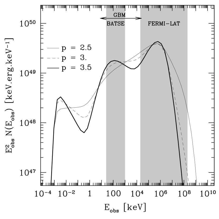
Figure 9: Effect of the slope of the accelerated electron distribution in the “inverse Compton case”. The observed spectrum (assuming $z=1$) obtained including all radiative processes is plotted for $\bar{\Gamma}=300$, $\kappa=4$, $\dot{E}=10^{52}\ \mathrm{erg\leavevmode\nobreak\ s^{-1}}$, $\tau=1\ \mathrm{s}$, $\epsilon_{\mathrm{B}}=10^{-3}$, $\epsilon_{\mathrm{e}}=1/3$, $\zeta=1$ and three different values of $p$. The first inverse Compton peak is well defined for $p>3$.

4.3 Dominant radiative process in the keV-MeV range and consequences at higher energy

From our exploration of the parameter space of the internal shock model we find, as expected from previous studies (Papathanassiou & Mészáros 1996; Daigne & Mochkovitch 1998; Mészáros & Rees 2000), that there are two classes of spectra, depending on the radiative process responsible for the prompt emission in the keV-MeV range. This energy range is detected for instance by instruments such as BATSE, Beppo-SAX, HETE-2, Integral, Swift or Fermi-GBM. These two cases have very different behavior in the MeV-GeV range and therefore Fermi-GBM+LAT observations will allow us to distinguish between the two possibilities.

“Synchrotron case”.

The synchrotron component peaks in the BATSE range (keV-MeV). This case is favored in internal shocks as it predicts pulse shapes and spectral evolution in GRB lightcurves that are in better agreement with observations (Daigne & Mochkovitch 1998, 2003). The “synchrotron case” is found in most spectra plotted in Fig. 8. In this case, the inverse Compton component peaks at higher energy (MeV-GeV range). These spectra are characterized by a high magentic field and by a low fraction $\zeta$ of accelerated electrons, which allows high values of the electron Lorentz factor $\Gamma_{\mathrm{m}}$. In the “synchrotron case” most inverse Compton scatterings occur in Klein-Nishina regime. This leads to four types of spectra at high energy (LAT range):

1. a strong second peak with a large $\gamma\gamma$ attenuation. This case is found for example for $\epsilon_{\mathrm{B}}\la 0.03$ in Fig. 8, panel (e);

2. a weak second peak with a negligible $\gamma\gamma$ attenuation. This case is found for example for $\bar{\Gamma}\sim 450-600$ in Fig. 8, panel (a);

3. a weak second peak with a strong $\gamma\gamma$ annihilation. This case is found for example for $\bar{\Gamma}\sim 250-450$ in Fig. 8, panel (a);

4. no second peak, the high-energy emission is only the tail of the synchrotron component, with a cutoff in the 100 MeV - 10 GeV range due to $\gamma\gamma$ annihilation. This case is found for example for $\bar{\Gamma}\la 250$ in Fig. 8, panel (a).

From case 1. to case 4., the bulk Lorentz factor $\bar{\Gamma}$ is decreasing, the contrast $\kappa$ is increasing, the injected kinetic power $\dot{E}$ is increasing, and/or the timescale $\tau$ is decreasing. We discuss below the corresponding possible physical diagnostics using Fermi data (§ 4.4).

Bulk Lorentz factor	Contrast
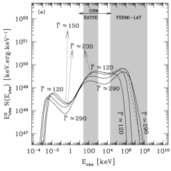
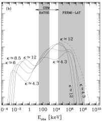
Injected kinetic power	Variability timescale

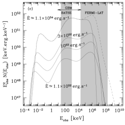
Figure 10: The effect of internal shock parameters on the emitted spectrum (“inverse Compton case”). Same as in Fig. 8 with a new “reference case” defined by $\bar{\Gamma}=300$, $\kappa=4$, $\dot{E}=10^{52}\ \mathrm{erg\leavevmode\nobreak\ s^{-1}}$, $\tau=1\ \mathrm{s}$, $\epsilon_{\mathrm{B}}=10^{-3}$, $\epsilon_{\mathrm{e}}=1/3$, $\zeta=1$ and $p=3.5$. (a) effect of $\bar{\Gamma}$. The transparency limit is reached for $\bar{\Gamma}\simeq 120$ and the efficiency limit for $\bar{\Gamma}\simeq 290$ ; (b) effect of $\kappa$. The efficiency limit is reached for $\kappa\simeq 4$ and the transparency limit for $\kappa\simeq 12$; (c) effect of $\dot{E}$. The efficiency limit is reached for $\dot{E}\simeq 1.1\times 10^{52}\ \mathrm{erg\leavevmode\nobreak\ s^{-1}}$ and the transparency limit is reached for $\dot{E}\simeq 1.1\times 10^{54}\ \mathrm{erg\leavevmode\nobreak\ s^{-1}}$; (d) effect of $\tau$. The transparency limit is reached for $\tau\simeq 0.01\ \mathrm{s}$ and the efficiency limit is reached for $\tau\simeq 0.9\ \mathrm{s}$. In each panel, the observed spectrum obtained without including $\gamma\gamma$ annihilation is plotted with a dashed line for the value of the parameter corresponding to the transparency limit.

“Synchrotron case”
High magnetic field	Low magnetic field
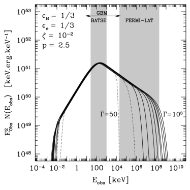
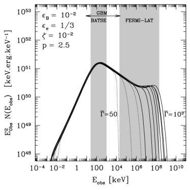
“Inverse Compton case”
High magnetic field	Low magnetic field

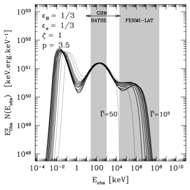
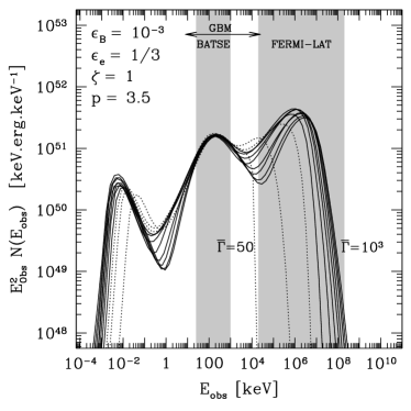
Figure 11: Physical diagnostics from Fermi observations: spectral shape. A GRB pulse at $z=1$ characterized by a peak energy $E_{\mathrm{p,obs}}=200\ \mathrm{keV}$, an isotropic radiated energy in the BATSE range $E_{\mathrm{25\,\mathrm{keV}-1\,\mathrm{MeV}}}=5\times 10^{51}\ \mathrm{erg}$ and a duration $(1+z)\tau=2\ \mathrm{s}$ is modelled using the two-shells version of the internal shock model and different assumptions for the microphysics. Top-left: “synchrotron case” with a high magnetic field ($\epsilon_{\mathrm{B}}=\epsilon_{\mathrm{e}}=1/3$, $\zeta=10^{-2}$ and $p=2.5$); Top-right: “synchrotron case” with a low magnetic field ($\epsilon_{\mathrm{B}}=10^{-2}$, $\epsilon_{\mathrm{e}}=1/3$, $\zeta=10^{-2}$ and $p=2.5$); Bottom-left: “ inverse Compton case” with a high magnetic field ($\epsilon_{\mathrm{B}}=\epsilon_{\mathrm{e}}=1/3$, $\zeta=1$ and $p=3.5$); Bottom-right: “ inverse Compton case” with a low magnetic field ($\epsilon_{\mathrm{B}}=10^{-3}$, $\epsilon_{\mathrm{e}}=1/3$, $\zeta=1$ and $p=3.5$). In each case, the evolution of the observed spectrum is plotted for an increasing bulk Lorentz factor $\bar{\Gamma}$ (calculation including all radiative processes), while the other parameters ($\kappa$, $\dot{E}$, $\tau$) are adjusted to match the imposed observed quantities. Spectra in dotted lines correspond to cases where pair creation should not be neglected ($\tau_{\mathrm{T}}^{\mathrm{tot}}>0.1$).

“Synchrotron case”		“Inverse Compton case”
High magnetic field	Low magnetic field	High magnetic field	Low magnetic field

Figure 12: Physical diagnostics from Fermi observations: properties of the relativistic outflow. For each case considered in Fig. 11, we plotted the values of the injected kinetic power $\dot{E}$ and the contrast $\kappa$ that have been adjusted for each bulk Lorentz factor $\bar{\Gamma}$ to match the imposed observed quantities (redshift $z=1$, peak energy $E_{\mathrm{p,obs}}=200\ \mathrm{keV}$, isotropic radiated energy $E_{\mathrm{25\ keV-1\ MeV}}=5\times 10^{51}\ \mathrm{erg}$ and duration $(1+z)\tau=2\ \mathrm{s}$). This adjustement is done within 10% uncertainty, which explains why the curves are not perfectly smooth. The corresponding typical internal shock radius $R_{\mathrm{is}}$ is also shown. The dotted lines correspond to cases where pair creation should not be neglected ($\tau_{\mathrm{T}}^{\mathrm{tot}}>0.1$).

“Inverse Compton case”.

The synchrotron component peaks at low energy and the inverse Compton component peaks in the BATSE range (keV-MeV). This case is usually called “Synchrotron Self-Compton” in the literature, and emerges naturally in the often considered situation where all electrons are accelerated ($\zeta=1$). It has been shown by Panaitescu & Mészáros (2000); Stern & Poutanen (2004) that it can reproduce the steep low-energy spectral slopes observed in the BATSE range. Because of the bright synchrotron component at low energy, possibly in the optical range, this case has recently been proposed to explain the prompt emission of the “naked eye burst” GRB 080319b (Racusin et al. 2008; Kumar & Panaitescu 2008) and more generally of bursts with a bright prompt optical emission (Panaitescu 2008). The “inverse Compton” case is characterized by a low magnetic field and a high fraction of accelerated electrons. In addition, having a well defined IC peak in the BATSE range requires a steep slope for the electron distribution, $p>3$ (see also Pe’er & Waxman 2004). While, the results obtained in the “synchrotron case” are very similar for all slopes $p>2$, we find a large difference in the “inverse Compton case” between spectra computed assuming a slope $2<p<3$ or assuming a slope $p>3$. It is only for $p>3$ that the first inverse Compton peak is well defined (the scatterings by electrons above $\Gamma_{\mathrm{p}}$ become negligible). This is illustrated in Fig. 9.

Fig. 10 shows the same parameter study as in Fig. 8, but for a reference set of parameters corresponding to the “inverse Compton case”. Note that the allowed range for each parameter $\bar{\Gamma}$, $\kappa$, $\dot{E}$ and $\tau$ is usually more limited than in the “synchrotron case”, especially due to the requirement of a high radiative efficiency ($u_{\mathrm{rad}}/u_{\mathrm{e}}^{\mathrm{acc}}>0.5$), as a lower magnetic field leads to longer synchrotron timescales. In the “inverse Compton case”, most scatterings occur in Thomson regime, due to a low magnetic field and a low minimum electron Lorentz factor leading to $\Gamma_{\mathrm{p}}\ll\Gamma_{\mathrm{KN}}$ (see Eq. (44)). The condition necessary to have the possibility of a second scattering in Thomson regime is $\Gamma_{\mathrm{p}}\epsilon_{\mathrm{p,ic}}\ll 1$, i.e.

$$\Gamma_{\mathrm{p}}\ll\Gamma_{\mathrm{KN}}^{\mathrm{(2^{nd})}}\simeq 200\left(\frac{B^{\prime}}{100\ \mathrm{G}}\right)^{-1/5}\ .$$ (62)

For most parameters in the “inverse Compton case” this condition is fulfilled and efficient second scatterings occur, leading to a second inverse Compton component at high energy (Fermi range). The first inverse Compton component is never affected by $\gamma\gamma$ annihilation. Therefore the spectra differ again mainly by their high-energy component, i.e. by the intensity of the second inverse Compton component. This intensity depends on whether most second scatterings occur in Thomson regime or are affected by Klein-Nishina corrections, and also on the strength of the attenuation due to $\gamma\gamma$ annihilation. As long as Klein-Nishina corrections and $\gamma\gamma$ absorption are not too strong at very high energy, the synchrotron, first and second inverse Compton components have relative intensities $1:Y:Y^{2}$, where $Y$ has to be large to avoid that most of the energy is radiated in the synchrotron component in the sub-keV range. Therefore, it is difficult to avoid that most of the energy is radiated in the MeV-GeV range. The isotropic equivalent radiated energy in the BATSE range is typically $E_{\mathrm{rad,BATSE}}\sim 10^{51}-10^{54}\ \mathrm{erg}$. If the Compton parameter is $Y\sim 10$ or more, the resulting total radiated energy is greater than $E_{\mathrm{rad}}\sim 10^{52}-10^{55}\ \mathrm{erg}$. This can lead to a crisis for the GRB energy budget and is another reason to disfavor the “inverse Compton case” as pointed out recently by Piran et al. (2008). High magnetic field can lead to smaller values of $Y$ but most of the energy is radiated in the synchrotron component in this case. Having the first inverse Compton peak dominant requires to fine-tune $\epsilon_{\mathrm{B}}$. Moreover the peak energy of the first inverse Compton component has a stronger dependence on the variations of the physical conditions in the shocked regions (compare Eqs. (34) and (43)). Thus the “inverse Compton case” also predicts a faster spectral evolution during GRB pulses than in the “synchrotron case” and is therefore disfavored by the observed pulse shape and spectral evolution in BATSE bursts (Daigne & Mochkovitch 1998, 2003).

4.4 Physical diagnostics from Fermi observations.

As can be seen from this study, the high-energy emission component is shaped by several physical parameters of the internal shock model. It is therefore difficult to identify simple diagnostics that could be applied to forthcoming Fermi data. It is only a detailed spectral fitting covering a broad spectral range that will allow us to measure fundamental quantities which are still largely unknown for GRBs (e.g. the radius and the Lorentz factor of the emitting material, the typical Lorentz factor of radiating electrons or the magnetic field in the shocked region).

Diagnosing the dominant radiative process and the physical conditions in the shocked region.

As seen in Fig. 11, one can distinguish between the “synchrotron case” and the ”inverse Compton case” from the spectral shape and then identify the dominant radiative process. This requires however a broad spectral range, like the one available with GBM+LAT. More precise informations about the physical conditions in the shocked region can be obtained from such observations using the following procedure: (a) assume microphysics parameters (the initial choice is suggested by the general spectral shape, for instance a high $\epsilon_{\mathrm{B}}$ and a low fraction $\zeta$ if the “synchrotron case” without bright IC component at high energy is favored); (b) estimate $\tau$ from the observed lightcurve; (c) vary $\bar{\Gamma}$ and for each $\bar{\Gamma}$ adjust $\kappa$ and $\dot{E}$ to match the correct observed peak energy and fluence in the BATSE range; (d) determine $\bar{\Gamma}$ from the spectral shape at high energy. This procedure is illustrated in Figs. 11 and 12. Good quality high energy observations can help in reducing the uncertainty related to the assumptions made for $\epsilon_{\mathrm{B}}$ and $\zeta$.

Figure 13: Measuring the Lorentz factor of the emitting region from the observed cutoff energy. The cutoff energy $E_{\mathrm{cut,obs}}$ due to $\gamma\gamma$ annihilation is plotted as a function of the Lorentz factor $\Gamma_{*}$ of the emitting region, as predicted from Eq. (LABEL:eq:cutoff), assuming $z=1$, $E_{\mathrm{rad,iso}}=5\times 10^{51}\ \mathrm{erg}$, $E_{\mathrm{p,obs}}=200\ \mathrm{keV}$ and $\beta=2.3$. The cutoff energies measured in all the spectra shown in Fig. 11 are indicated with four different symbols corresponding to the four different assumptions regarding the microphysics parameters.

Measuring the Lorentz factor of the outflow.

It has been proposed by several authors to measure the Lorentz factor of the relativistic outflow from the position of the cutoff in the high energy spectrum due to $\gamma\gamma$ annihilation (see e.g. Baring & Harding 1997; Lithwick & Sari 2001; Baring 2006; Gupta & Zhang 2008; Murase & Ioka 2008). It is assumed that three quantities have been measured: the isotropic equivalent radiated energy $E_{\mathrm{rad,iso}}$, the peak energy $E_{\mathrm{p,obs}}$ and the typical pulse duration $\tau_{\mathrm{obs}}=(1+z)\tau$. From Sect. 1, the radius where the emission takes place is related to the unknown Lorentz factor of the emitting region $\Gamma_{*}$ by $R=2\kappa^{2}/(\kappa^{2}-1)\Gamma_{*}^{2}c\tau\simeq 2\Gamma_{*}^{2}c\tau$ (the difference is less than 10% for $\kappa>3$). The comoving photon density can then be estimated as a function of $\Gamma_{*}$ :

$$n^{\prime}\left(E^{\prime}\right)\simeq\frac{\Gamma_{*}E_{\mathrm{rad,iso}}}{4\pi R^{2}\left(1+z\right)^{2}E_{\mathrm{p,obs}}^{2}\Delta^{\prime}}\left(\frac{\Gamma_{*}E^{\prime}}{(1+z)E_{\mathrm{p,obs}}}\right)^{-\beta}\ ,$$ (63)

where $-\beta$ is the observed slope of the photon spectrum in the BATSE range and $\Delta^{\prime}$ is the comoving width of the emitting region. Using the Dirac approximation for the $\gamma\gamma$ annihilation cross section (Gould & Schréder 1967), one gets the following expression for the optical depth at observed energy $E_{\mathrm{obs}}$ :

$$\tau_{\mathrm{\gamma\gamma}}\left(E_{\mathrm{obs}}\right)\simeq\sigma_{\mathrm{T}}\Delta^{\prime}\frac{\Gamma_{*}\left(m_{\mathrm{e}}c^{2}\right)^{2}}{(1+z)E_{\mathrm{obs}}}n^{\prime}\left(E^{\prime}=\frac{\Gamma_{*}\left(m_{\mathrm{e}}c^{2}\right)^{2}}{(1+z)E_{\mathrm{obs}}}\right)\ .$$ (64)

The cutoff energy can be estimated from the condition $\tau_{\mathrm{\gamma\gamma}}\left(E_{\mathrm{cut,obs}}\right)\sim 1$, which gives

$$E_{\mathrm{cut,obs}} \simeq \frac{m_{\mathrm{e}}c^{2}}{1+z}\left(\frac{(1+z)^{2}\sigma_{\mathrm{T}}E_{\mathrm{rad,iso}}}{16\pi m_{\mathrm{e}}c^{4}\tau_{\mathrm{obs}}^{2}}\right)^{-\frac{1}{\beta-1}}\Gamma_{*}^{2\frac{\beta+1}{\beta-1}}\left(\frac{(1+z)E_{\mathrm{p,obs}}}{m_{\mathrm{e}}c^{2}}\right)^{-\frac{\beta-2}{\beta-1}}\ .$$

This estimate of the observed cutoff energy $E_{\mathrm{cut,off}}$ is plotted as a function of the Lorentz factor $\Gamma_{*}$ of the emitting material in Fig. 13 for the same observed quantities as in Fig. 11, i.e. $z=1$, $E_{\mathrm{rad,iso}}=5\times 10^{51}\ \mathrm{erg}$, $E_{\mathrm{p,obs}}=200\ \mathrm{keV}$ and $\tau_{\mathrm{obs}}=2\ \mathrm{s}$, and assuming a slope $\beta=2.3$ (note that – for most of the values of the cutoff energy $E_{\mathrm{cut,obs}}$ plotted in Fig. 13 – the typical energy $\sim\Gamma_{*}^{2}\left(m_{\mathrm{e}}c^{2}\right)^{2}/(1+z)^{2}/E_{\mathrm{cut,obs}}$ of low-energy photons that annihilate preferentially with photons at energy $E_{\mathrm{cut,obs}}$ is above $E_{\mathrm{p,obs}}$, which justifies our choice of $\beta$). On the same figure the measured values of $E_{\mathrm{cut,obs}}$ are plotted for all spectra shown in Fig. 11, i.e. for three different cases regarding the microphysics. This cutoff energy is measured as the energy where the slope of the photon spectrum falls below -3. It appears that the precise calculation agrees well with the approximate expression given by Eq. (LABEL:eq:cutoff) in the “synchrotron case” (except for a normalization factor of about $\sim 3$, which could be improved with a more accurate description of the low energy spectrum in equation 63) but that there is a large discrepancy in the “inverse Compton case” where Eq. (LABEL:eq:cutoff) overestimates $E_{\mathrm{cut,obs}}$. The $\gamma\gamma$ annihilation in this case is indeed negligible and the cutoff observed at high energy is due to the limitation of inverse Compton scatterings by Klein-Nishina corrections.

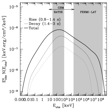
Figure 14: A single pulse burst in the “synchrotron case” with a high magnetic field. The dynamics is the same as in Fig. 1 except for $\dot{E}=5\times 10^{53}\ \mathrm{erg\leavevmode\nobreak\ s^{-1}}$. The assumed microphysics parameters are $\epsilon_{\mathrm{B}}=\epsilon_{\mathrm{e}}=1/3$, $\zeta=3\times 10^{-3}$ and $p=2.5$. All radiative processes are included in the calculation. Left: observed lightcurves in Fermi-GBM and LAT range. The synchrotron (thin solid line) and inverse Compton (thin dashed line) components are also shown. Right: observed time-integrated spectrum during the rise, the early decay and the whole duration of the pulse.

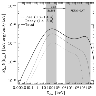
Figure 15: A single pulse burst in the “synchrotron case” with a low magnetic field. Same as in Fig. 14 except for the microphysics parameters: $\epsilon_{\mathrm{B}}=5\times 10^{-3}$, $\epsilon_{\mathrm{e}}=1/3$, $\zeta=2\times 10^{-3}$ and $p=2.5$.

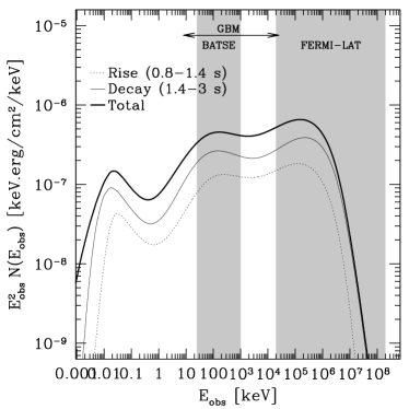
Figure 16: A single pulse burst in the “inverse Compton case”. Same as in Fig. 14 except for the initial distribution of the Lorentz factor that varies from 100 to 600 and for the microphysics parameters: $\epsilon_{\mathrm{B}}=10^{-2}$, $\epsilon_{\mathrm{e}}=1/3$, $\zeta=1$ and $p=3.5$. In the left panel, the lightcurves observed both in the Fermi-GBM+LAT energy range are entirely dominated by inverse Compton emission.

From this study, it appears that using estimate of the Lorentz factor from the observed cutoff energy such as Eq. (LABEL:eq:cutoff) is acceptable when the high-energy spectrum does not show any new bright component in addition to the low-energy spectrum. To confirm any value of the Lorentz factor measured by this method, one should do a detailed modelling of the spectrum to check whether the process responsible for the observed cutoff has been correctly identified. Note that the emission from electron–positron pairs created by $\gamma\gamma$ annihilation is not included here and that it could provide additional diagnostics (Murase & Ioka 2008). Note also that the final shape of the spectrum above the cutoff energy can become complicated when considering the spectrum integrated over the whole duration of a pulse, as we show in the next section (see also the detailed discussion by Granot et al. 2008). It can make the diagnostics more difficult and emphasizes again the necessity of a detailed modelling.

5 Observed time profiles and spectra

All the spectra shown in the previous section are computed for a “typical collision”, using the two shell version of the internal shock model. However even for a single pulse, the emission radius, and the physical conditions in the shocked medium, can span several orders of magnitude during the propagation of the “internal shock” waves (see Fig. 1). This leads to a spectral evolution during the observed pulse that is entirely missed by the two shell model. In the present section, we show examples of synthetic bursts computed by coupling the detailed model for the dynamics of the relativistic outflow (§ Sect. 2.1) with the radiative code (§ Sect. 2.3), and we discuss the predicted spectral evolution, as well as the high energy emission (Fermi-LAT range). In all examples, a redshift $z=1$ is assumed.

5.1 A single pulse burst

We present three synthetic single pulse bursts corresponding to the same relativistic outflow : a total duration of the relativistic ejection phase $t_{\mathrm{w}}=2\ \mathrm{s}$, a Lorentz factor varying from 100 to 400 during the ejection as in Fig. 1 and $\dot{E}=5\times 10^{53}\ \mathrm{erg\leavevmode\nobreak\ s^{-1}}$. The dynamics is computed using a discretization of the outflow in $1000$ shells. The three cases differ by different sets of microphysics parameters : (i) “synchrotron case” with a high magnetic field (see Fig. 14), $\epsilon_{\mathrm{B}}=\epsilon_{\mathrm{e}}=1/3$, $\zeta=3\times 10^{-3}$ and $p=2.5$ ; (ii) “synchrotron case” with a low magnetic field (see Fig. 15), $\epsilon_{\mathrm{B}}=5\times 10^{-3}$, $\epsilon_{\mathrm{e}}=1/3$, $\zeta=2\times 10^{-3}$ and $p=2.5$ ; (iii) “inverse Compton case” (see Fig. 16), $\epsilon_{\mathrm{B}}=10^{-2}$, $\epsilon_{\mathrm{e}}=1/3$, $\zeta=1$ and $p=3.5$. In this last case, the contrast $\kappa=\Gamma_{\mathrm{max}}/\Gamma_{\mathrm{min}}$ of the initial distribution of the Lorentz factor has been increased ($\Gamma$ varies from 100 to 600 instead of 400) to increase the dynamical efficiency, and thus compensate for a lower radiative efficiency (as well as a lower fraction of the emission that is radiated in the Fermi-GBM range). The three pulses have comparable isotropic equivalent energies radiated in the GBM range. The lightcurves in the GBM+LAT range are plotted for each case, as well as the time-integrated spectrum during the rise, the decay and the whole duration of the pulse. GRB lightcurves in the keV-MeV range usually show a hard-to-soft evolution (see e.g. Bhat et al. 1994; Ford et al. 1995; Norris et al. 1996). This spectral evolution is found in these three examples of synthetic GRBs, as the spectrum during the rise peaks at higher energy than during the decay phase.

In the GBM range, the three lightcurves are quite similar, except for a faster pulse decay in the inverse Compton case. We checked in the three cases that the expected spectral evolution (see e.g. Norris et al. 1996) in the keV-MeV range is reproduced, in agreement with the previous results of Daigne & Mochkovitch (1998): the photon flux peaks earlier at higher energy and the duration of the pulse increases at lower energies.

In the LAT range on the other hand, the spectral evolution and the corresponding behavior at high energy are different in the three considered cases. In the “synchrotron case”, the physical process responsible for the radiation is not the same in the GBM range (synchrotron) and in the LAT range (synchrotron+possible additional inverse Compton component, depending on the intensity of the magnetic field). Therefore, the lightcurves at low and high-energy do not look similar. In particular, the inverse Compton component at high energy emerges later than the synchrotron component, increasing the duration of the pulse in the LAT range. It is due to an evolving Compton parameter during the pulse duration. This effect is more important when inverse Compton scatterings become more efficient (compare Figs. 14 and 15). For the lowest values of $\epsilon_{\mathrm{B}}$, the lightcurve at high energy could even peak with a delay with respect to the lightcurve in the GBM range if the inverse Compton component becomes more intense that the synchrotron component in the high energy range. This behavior of the LAT lightcurves is due to the evolution of the physical condition in the shocked medium along the propagation of the shock wave. It is illustrated in Fig. 17, where the ratio of the inverse Compton over the synchrotron component is plotted as a function of the observer time, as well as the dynamical timescale $t^{\prime}_{\mathrm{ex}}$ and the synchrotron timescale $t^{\prime}_{\mathrm{syn}}$ :

Figure 17: A single pulse burst in the “synchrotron case” with a low magnetic field: dynamical evolution during the pulse. The evolution of the synchrotron timescale, the dynamical timescale and the ratio of the energy radiated in the inverse Compton over the energy radiated in the synchrotron component is plotted as a function of the observer time for the synthetic single pulse burst shown in Fig. 15.

• Initially, due to the shape adopted for the initial distribution of the Lorentz factor in the outflow, the shock is weak and the dissipated energy per particle is low. This results in moderate electron Lorentz factors $\Gamma_{\mathrm{m}}$, and therefore large synchrotron timescales. On the other hand, these early times correspond to small radii so the dynamical timescale is still small. In this first phase, $t^{\prime}_{\mathrm{syn}}\la t^{\prime}_{\mathrm{ex}}$ and the efficiency of inverse Compton scatterings is large, as a large fraction of the shocked region is populated by relativistic electrons (see Sect. 3). It results in a weak precursor in the GeV lightcurve. This precursor can disappear if a different initial distribution of the Lorentz factor in the outflow is adopted, especially if it leads to an immediate violent shock (for instance with an initial discontinuity).

• In a second phase (around the peak of the pulse in the GBM range), the shock becomes stronger, $\Gamma_{\mathrm{m}}$ increases and the synchrotron timescale decreases. On the other hand, as the radius increases, the dynamical timescale increases. This results in $t^{\prime}_{\mathrm{syn}}\ll t^{\prime}_{\mathrm{ex}}$ and a low efficiency for inverse Compton scatterings. The emission at high energy is dominated by the synchrotron component.

• A late times (tail of the pulse), the synchrotron timescale increases again (mainly due to the decrease of the magnetic field as the radius increases) and the efficiency of inverse Compton scatterings increases again. The inverse Compton component becomes dominant again in the GeV range, which results in a prominent GeV tail of the pulse.

On the other hand, in the “inverse Compton case”, inverse Compton scatterings are the dominant radiative process both in the GBM and the LAT range. Therefore, the lightcurves are much more similar in the different energy bands.

It appears clearly from Figs. 14, 15 and 16 that in addition to the time-integrated spectrum, the observed spectral evolution and the comparison of the GBM and LAT lightcurves are also powerful tools to diagnose the dominant radiative process and the physical conditions in the shocked medium (electron distribution and magnetic field).

5.2 A multi-pulses GRB

Fig. 19 shows two examples of more complex synthetic GRBs. The dynamical evolution is the same in both cases, assuming the initial distribution of the Lorentz factor plotted in Fig. 18, which leads to 4 main pulses in the lightcurve. It is computed using a discretization of the outflow in $4000$ shells. The two examples correspond to two different sets of microphysics parameters (“synchrotron case” with a high or a low magnetic field). These examples illustrate that in a complex burst, each pulse exhibits a hard to soft evolution in the main spectral component and that – when possible – the spectral analysis should be made by integrating the spectrum over a pulse rather than over the whole duration of the GRB. The spectral evolution and the behaviour at high energy that were identified for single pulse burst are also observed in these multi-pulse GRBs. In particular, the lightcurve above 1 GeV in the “synchrotron case” with a low magnetic field shows more flat topped pulses and prolonged emission in the pulse decays.

Figure 18: An example of a multi-pulses burst : initial distribution of the Lorentz factor in the relativistic outflow. The initial Lorentz factor in the outflow is plotted as a function of the ejection time (top axis) or equivalently the distance from the source at the end of the ejection phase (bottom axis).

Figure 19: An example of a multi-pulses burst : lightcurves. The dynamics is computed for the initial distribution of the Lorentz factor plotted in Fig. 18, assuming a total duration of the relativistic ejection phase $t_{\mathrm{w}}=8\ \mathrm{s}$ and an injected kinetic power $\dot{E}=5\times 10^{53}\ \mathrm{erg\,s^{-1}}$. The two examples differ by the assumptions for the microphysics parameters.Left: “synchrotron case” with a high magnetic field. The microphysics parameters are $\epsilon_{\mathrm{B}}=\epsilon_{\mathrm{e}}=1/3$, $\zeta=0.002$ and $p=2.5$. The observed peak energy of the spectrum integrated over the whole duration of the burst is $\sim 180\ \mathrm{keV}$. Right: “synchrotron case” with a low magnetic field. The microphysics parameters are $\epsilon_{\mathrm{B}}=8\times 10^{-4}$, $\epsilon_{\mathrm{e}}=1/3$, $\zeta=0.001$ and $p=2.5$. The observed peak energy is $\sim 250\ \mathrm{keV}$. In both cases the lightcurves are plotted in different energy channels (Fermi-GBM+LAT) assuming a redshift $z=1$.

6 Conclusions

We have developed a detailed model for the prompt emission of gamma-ray bursts in the framework of the internal shock model. It combines dynamical simulations that follow the evolution of the physical conditions (Lorentz factor, density and energy density) in the shocked regions along the propagation of “internal” shock waves in the relativistic outflow, and a time-dependant radiative code to compute the emission from shock-accelerated electrons, including the most relevant processes (adiabatic cooling, synchrotron radiation and self-absorption, inverse Compton scatterings and photon–photon annihilation). We have used our model to explore the parameter space of the internal shock model and identify physical diagnostics for Fermi data.

We list here our main results:

1. The comparison of the results of the radiative code with standard analytical or semi-analytical estimates of the emitted spectrum shows that the synchrotron component is usually well predicted by the analytical spectrum from Sari et al. (1998), except when inverse Compton scatterings become efficient.

2. We show that the prediction of the high-energy component based on the time-averaged electron distribution and the time-averaged synchrotron photon spectrum (e.g. Sari & Esin 2001) is less precise, especially above the peak of the inverse Compton component. The accuracy of this time-averaged prediction decreases as the efficiency of inverse Compton scatterings increases. This is mainly due to time-dependent effects : time-averaged distributions do not take into account the time needed to build the photon field.

   Table 1: Physical diagnostics for Fermi data:

   Observational constraints :
   –Is there an additional component in the LAT spectrum ?	no (or very weak)	yes	yes (possibly very intense)
   –Is the LAT lightcurve in GeV range prolonged or delayed compared to GBM lightcurve ?	yes (tail)	yes (delayed peak)	no (or very short delay)
   Consequences:
   Radiative processes:
   Dominant process in GBM range	synchrotron	synchrotron	IC (first peak)
   Dominant process in LAT range	synchrotron + very weak IC	synchrotron + IC	IC (second peak)
   Conditions in shocked regions:
   Electron distribution	high $\Gamma_{\mathrm{m}}$, low $\zeta$	high $\Gamma_{\mathrm{m}}$, low $\zeta$	moderate $\Gamma_{\mathrm{m}}$, $\zeta\to 1$
   Magnetic field	high ($\epsilon_{\mathrm{B}}\to 1/3$)	low ($\epsilon_{\mathrm{B}}\ll 1$)	low ($\epsilon_{\mathrm{B}}\ll 1$)
   Properties of the relativistic outflow:
   Can the Lorentz factor in the outflow be measured from the high-energy cutoff (assuming it is due to $\gamma\gamma$ annihilation) ?	yes	yes	? (see text)

   These diagnostics are based on the results shown in Sect. 4 and 5.

3. An important consequence of the previous result is that the electron cooling rate, and therefore the time-averaged electron distribution, is not correctly predicted by the standard analytical estimate from Sari et al. (1998) when inverse Compton scatterings become important. This affects the spectral shape of the synchrotron component as well. We find that the resulting spectral slope (photon spectrum) below the peak energy is steeper than the usual value $-3/2$ in synchrotron fast cooling regime, in agreement with Derishev et al. (2001) who shows that the slope can become as steep as $-1$ when Klein-Nishina corrections are important. This may reconcile the synchrotron radiation with the observed distribution of the low-energy slope $\alpha$ in BATSE (Preece et al. 2000; Kaneko et al. 2006) and HETE-2 (Sakamoto et al. 2005) bursts. We will investigate this question in a forthcoming paper.

4. When exploring the parameter space of internal shocks, we find that two classes of broad-band spectra can be expected, which correspond to different physical conditions in the shocked region :

   • ”Synchrotron case”, where the dominant process in the Fermi-GBM range is synchrotron radiation. It requires high electron Lorentz factors and therefore implies that only a fraction of the electrons are shock-accelerated. The intensity of the inverse Compton component in the LAT range depends on the intensity of the magnetic field but remains always limited due to Klein-Nishina corrections. A high-energy cutoff is present due to photon-photon annihilation, which allows us to estimate the Lorentz factor of the emitting material. As the high-energy lightcurve is made of two different components (synchrotron + inverse Compton) whose ratio evolves during a pulse, the lightcurves can differ in the GBM and the LAT range. In particular, for low $\epsilon_{\mathrm{B}}/\epsilon_{\mathrm{e}}$ ratios that favor inverse Compton scatterings, a pulse in the GBM can be followed by a tail of GeV photon in the LAT. When there is a significant inverse Compton component in the LAT, the pulse above 1 GeV can even peak with a delay compared to the GBM.

   • ”Inverse Compton case”, where the synchrotron component peaks at low energy and the dominant process in the GBM range is inverse Compton. A second inverse Compton peak is usually present at higher energy but further scatterings are suppressed by Klein-Nishina corrections. The cutoff at high energy can be either due to $\gamma\gamma$ annihilation or to the Klein-Nishina suppression of inverse Compton scatterings, which makes more difficult to estimate the Lorentz factor of the emitting material in this case. A steep slope for the electron distribution is necessary to have two well distinct peaks in the inverse Compton component. The relative intensity of the synchrotron and the two inverse Compton peaks in the spectrum depends on the ratio $\epsilon_{\mathrm{e}}/\epsilon_{\mathrm{B}}$. It requires some fine-tuning to have a dominant first inverse Compton peak in the GBM range, which can lead to a energy crisis (Piran et al. 2008). As the emission detected in the GBM and LAT lightcurves is due to the same process (inverse Compton), the lightcurves in the two instruments are much more similar.

5. This study allows us to define physical diagnostics for Fermi data, based on the spectral shape and the spectral evolution, that are summarized in Tab. 1. We plan to apply these diagnostics as soon as Fermi GRB data will be made public. Our study emphasizes however that a detailed broad-band spectral modelling is always necessary to reach firm conclusions regarding the properties of the outflow and the physical conditions in the shocked regions.

Several arguments (energetics, spectral evolution) already favor the “synchrotron case”. Bursts detected by Fermi both by the GBM and the LAT should allow us to firmly distinguish these two possibilities and show if all bursts are in the ”synchrotron case” or if the ”inverse Compton case” can also be found.

In the “synchrotron case”, it is assumed that only a fraction of the electrons is accelerated to very high Lorentz factors ($\Gamma_{\mathrm{m}}\sim 10^{4}$). If a small fraction of the dissipated energy in the shock is injected in the remaining electrons, they will have a Maxwellian distribution with a mean Lorentz factor of a few. We will investigate in a future work what could be the contribution of these electrons to the emission and more generally discuss the prompt optical emission of GRBs in the framework of the internal shock model.

Appendix A Radiative processes

We list here the source and loss terms appearing in the equations governing the evolution of the electron distribution (Eq. (15)) and of the photon spectrum (Eq. (16)).

A.1 Adiabatic cooling

$$\left.\frac{d\gamma}{dt^{\prime}}\right|_{\mathrm{ad}}=-\frac{\gamma}{t^{\prime}_{\mathrm{ex}}}\ .$$ (66)

A.2 Synchrotron emission

We assume an isotropic distribution for the pitch angle $\alpha$ between the electron velocity and the magnetic field, so that $\left\langle\sin^{2}{\alpha}\right\rangle=2/3$. The synchrotron power is given by Rybicki & Lightman (1979) and leads to

$$\left.\frac{d\gamma}{dt^{\prime}}\right|_{\mathrm{syn}} = -\frac{\sigma_{\mathrm{T}}}{6\pi m_{\mathrm{e}}c}B^{2}\gamma^{2}\ ,$$ (67)

$$P^{\mathrm{syn}}_{\nu^{\prime}}\left(\gamma\right) = \frac{\sigma_{\mathrm{T}}m_{\mathrm{e}}c^{2}}{3e}B\ \Phi\left(\frac{\nu^{\prime}}{\nu^{\prime}_{\mathrm{syn}}\left(\gamma\right)}\right)\ ,$$ (68)

where the synchrotron frequency is defined by

$$\nu_{\mathrm{syn}}\left(\gamma\right)=\frac{3e}{4\pi m_{\mathrm{e}}c}B\gamma^{2}$$ (69)

and the function $\Phi$ is defined by

$$\Phi\left(x\right)=\frac{9\sqrt{3}}{8\pi}x\int_{x}^{+\infty}\mathrm{d}u\,K_{5/3}(u)\ .$$ (70)

This definition has been chosen so that $\int_{0}^{+\infty}\mathrm{d}x\,\Phi(x)=1$.

A.3 Synchrotron self-absorption

The cross-section is given by Rybicki & Lightman (1979):

$$\sigma_{\mathrm{sa}}\left(\gamma,\nu^{\prime}\right)=\frac{1}{8\pi m_{\mathrm{e}}\left.\nu^{\prime}\right.^{2}}\frac{P^{\mathrm{syn}}_{\nu^{\prime}}\left(\gamma\right)}{\gamma}\left[2-\frac{\partial\ln{n}}{\partial\ln{\gamma}}\left(\gamma,t^{\prime}\right)\right]\ .$$ (71)

In the present version of our radiative code, the corresponding source term $\left.d\gamma/dt^{\prime}\right|_{\mathrm{sa}}$ is not included in the equation for the evolution of electrons (Eq. (15)).

A.4 Inverse Compton scatterings

We use the kernel derived by Jones (1968), which has an excellent accuracy, even in the Klein-Nishina regime.

$$\left.\frac{d\gamma}{dt^{\prime}}\right|_{\mathrm{ic}} = -\frac{3}{4}\frac{h\sigma_{\mathrm{T}}}{m_{\mathrm{e}}c}\frac{1}{\gamma^{2}}\int\mathrm{d}\nu^{\prime}\,\nu^{\prime}\int\frac{\mathrm{d}\tilde{\nu}^{\prime}}{\tilde{\nu}^{\prime}}n_{\tilde{\nu}^{\prime}}(t^{\prime})K\left(\gamma,\nu^{\prime},\tilde{\nu}^{\prime}\right)\ ,$$ (72)

$$P^{\mathrm{ic}}_{\nu^{\prime}} = \frac{3}{4}h\sigma_{\mathrm{T}}c\frac{\nu^{\prime}}{\gamma^{2}}\int\frac{\mathrm{d}\tilde{\nu}^{\prime}}{\tilde{\nu}^{\prime}}n_{\tilde{\nu}^{\prime}}(t^{\prime})K\left(\gamma,\nu^{\prime},\tilde{\nu}^{\prime}\right)$$ (73)

with

$$K\left(\gamma,\nu^{\prime},\tilde{\nu}^{\prime}\right) = \frac{\epsilon}{\tilde{\epsilon}}-\frac{1}{4\gamma^{2}}\ \mathrm{if}\ \frac{\tilde{\epsilon}}{4\gamma^{2}}<\epsilon<\tilde{\epsilon}\ ,$$ (74)

$$= 2q\ln{q}+\left(1+2q\right)\left(1-q\right)+\frac{1}{2}\left(1-q\right)\frac{\left(4\gamma\tilde{\epsilon}q\right)^{2}}{1+4\gamma\tilde{\epsilon}q}$$

$$\mathrm{if}\ \tilde{\epsilon}<\epsilon<\frac{4\gamma^{2}\tilde{\epsilon}}{1+4\gamma\tilde{\epsilon}}\ ,$$

where $\epsilon=h\nu^{\prime}/m_{\mathrm{e}}c^{2}$, $\tilde{\epsilon}=h\tilde{\nu}^{\prime}/m_{\mathrm{e}}c^{2}$ and $q=\epsilon/4\gamma\tilde{\epsilon}/\left(\gamma-\epsilon\right)$ . In the present version of the code, the corresponding loss term

$$\left.\frac{\partial n_{\nu^{\prime}}}{\partial t^{\prime}}\right|_{\mathrm{ic,loss}}=-cn_{\nu^{\prime}}(t^{\prime})\int\mathrm{d}\gamma\,n\left(\gamma,t^{\prime}\right)\sigma_{\mathrm{ic}}\left(\gamma,\nu^{\prime}\right)$$

is not included in the right-hand part of the equation for the evolution of photons (Eq. (16)). For this reason, we can not compute the emitted spectrum when $\tau_{\mathrm{T}}^{\mathrm{acc}}\ga 1$ and can not reproduce a Comptonized spectrum.

A.5 Photon–photon annihilation

We use the exact cross section given by Gould & Schréder (1967) for an isotropic photon field, which is a good approximation as long as the radiative timescale is small compared to the dynamical timescale (see Sect. 2.3).

$$\sigma_{\mathrm{\gamma\gamma}}\left(\nu^{\prime},\tilde{\nu}^{\prime}\right) = \left[\frac{1+\beta^{2}}{1-\beta^{2}}-\beta^{2}-\ln{\frac{1+\beta}{1-\beta}}+4\ln{\frac{2}{1-\beta}}\right]\ln{\frac{1+\beta}{1-\beta}}$$ (75)

$$-\frac{4\beta}{1-\beta^{2}}+2\beta-\int_{1}^{(1+\beta)/(1-\beta)}\frac{\mathrm{d}x}{x}\,\ln{\left(1+x\right)}\ ,$$

where

$$\beta=\sqrt{\frac{h\nu^{\prime}h\tilde{\nu}^{\prime}-\left(m_{\mathrm{e}}c^{2}\right)^{2}}{h\nu^{\prime}h\tilde{\nu}^{\prime}}}\ .$$

In the present version of the code, the source and loss terms due to pair production and pair annihilation are not included in Eq. (15), and the associated radiation is not included in Eq. (16).

Appendix B Numerical method

To solve the system of the two Eqs. (15) and (16) for the evolution of the electron distribution $n\left(\gamma,t^{\prime}\right)$ and the photon spectrum $n_{\nu^{\prime}}(t^{\prime})$ in the comoving frame of the shocked material, we have developed a numerical scheme that is a good compromise between accuracy and computing speed. We use normalized variables $\tilde{t}=t^{\prime}/t^{\prime}_{\mathrm{ex}}$, $\epsilon=h\nu^{\prime}/m_{\mathrm{e}}c^{2}$, $\tilde{n}\left(\gamma,\tilde{t}\right)=n\left(\gamma,t\right)/n_{\mathrm{e}}^{\mathrm{acc}}$ and $\tilde{n}_{\epsilon}(\tilde{t})=\left(m_{\mathrm{e}}c^{2}/h\right)n_{\nu^{\prime}}(t^{\prime})/n_{\mathrm{e}}^{\mathrm{acc}}$. The photon spectrum at time $\tilde{t}_{\mathrm{k}}$ after the $\mathrm{k}^{\mathrm{th}}$ step is stored in a fixed grid $\epsilon_{\mathrm{j}}$ for $j=1\to M$, i.e. $\tilde{n}_{\mathrm{j}}^{\mathrm{(k)}}=\tilde{n}_{\epsilon_{\mathrm{j}}}\left(\tilde{t}_{\mathrm{k}}\right)$. At $\tilde{t}=0$, no photons are present so that $\tilde{n}_{\mathrm{j}}(0)=0$. To take advantage of the short radiative timescale, the electron distribution at time $t_{\mathrm{k}}$ is stored in a moving (“Lagrangian”) grid $\gamma_{\mathrm{i}}^{\mathrm{(k)}}=\gamma_{\mathrm{i}}\left(\tilde{t}_{\mathrm{k}}\right)$ for $i=0\to N$, i.e.

$$\Delta\tilde{n}_{\mathrm{i}}^{\mathrm{(k)}}=\int_{\gamma_{\mathrm{i-1}}^{\mathrm{(k)}}}^{\gamma_{\mathrm{i}}^{\mathrm{(k)}}}\mathrm{d}\gamma\,\tilde{n}\left(\gamma,\tilde{t}\right)\ .$$

This insures that the number of electrons is exactly conserved. At $\tilde{t}=0$, this grid is adjusted to the distribution of accelerated electrons given by Eq. (5), i.e. $\gamma_{0}^{\mathrm{(0)}}=\Gamma_{\mathrm{m}}$, $\gamma_{N}^{\mathrm{(0)}}=\Gamma_{\mathrm{M}}$ and $\Delta\tilde{n}_{\mathrm{i}}^{\mathrm{(0)}}=\left(\gamma_{\mathrm{i-1}}^{\mathrm{(0)}}/\Gamma_{\mathrm{m}}\right)^{1-p}-\left(\gamma_{\mathrm{i}}^{\mathrm{(0)}}/\Gamma_{\mathrm{m}}\right)^{1-p}$. In practice, all results presented in this paper are obtained using logarithmic grids for $\epsilon_{\mathrm{j}}$ and $\gamma_{\mathrm{i}}^{\mathrm{(0)}}$ with $N=M=100$. The time-evolution of $\tilde{n}_{\mathrm{j}}^{\mathrm{(k)}}$ is computed using a discretized version of Eq. (16). On the other hand, to compute the time-evolution of $\gamma_{\mathrm{i}}^{\mathrm{(k)}}$, we replace Eq. (15) by

$$\frac{d\gamma}{d\tilde{t}}\left(\tilde{t}\right)=t^{\prime}_{\mathrm{ex}}\left(\left.\frac{d\gamma}{dt^{\prime}}\right|_{\mathrm{ad}}+\left.\frac{d\gamma}{dt^{\prime}}\right|_{\mathrm{syn}}+\left.\frac{d\gamma}{dt^{\prime}}\right|_{\mathrm{ic}}\right)\ .$$ (76)

In fast cooling regime the values of $\gamma_{\mathrm{i}}^{\mathrm{(k)}}$ decrease rapidly, which is a valuable advantage, as the timestep of the simulation is given by the radiative timescale of the most energetic electrons still present in the medium. We observe a rapid increase of the timestep following the cooling of the electrons, and reach therefore $\tilde{t}=1$ in a small number of steps. In addition, as $-d\gamma/d\tilde{t}$ is an increasing function of $\gamma$, the width of each cell in the electron grid ($\gamma_{\mathrm{i}}^{\mathrm{(k)}}-\gamma_{\mathrm{i-1}}^{\mathrm{(k)}}$) is decreasing with time, which allows at the end of the simulation to merge cells of cooled electrons and therefore gain an additional reduction of the computing time. Energy is not necessarily conserved in our code due to the finite size of the electron and photon grids: typically, the error is a few percents and is never larger than 10 %.

Appendix C Formation of the radiation field: the Compton parameter $Y(t^{\prime})$.

When only adiabatic cooling and synchrotron radiation are considered, the equation for the evolution of electrons has a simple analytic solution, given by

$$n\left(\gamma,t^{\prime}\right)=\left(\frac{\gamma_{0}\left(\gamma,t^{\prime}\right)}{\gamma}\right)^{2}n\left(\gamma_{0}\left(\gamma,t^{\prime}\right),t^{\prime}=0\right)\ ,$$ (77)

where $\gamma_{0}\left(\gamma,t^{\prime}\right)$ is the initial Lorentz factor at $t^{\prime}=0$ of an electron having cooled to the Lorentz factor $\gamma$ at time $t^{\prime}$, i.e.

$$\gamma_{0}\left(\gamma,t^{\prime}\right)=\frac{\Gamma_{\mathrm{c}}}{\left(1+\frac{\Gamma_{\mathrm{c}}}{\gamma}\right)e^{-t^{\prime}/t^{\prime}_{\mathrm{ex}}}-1}\ .$$ (78)

At time $t^{\prime}$, electrons have Lorentz factors in the interval

$$\Gamma_{\mathrm{m}}(t^{\prime})=\frac{\Gamma_{\mathrm{c}}}{\left(1+\frac{\Gamma_{\mathrm{c}}}{\Gamma_{\mathrm{m}}}\right)e^{t^{\prime}/t^{\prime}_{\mathrm{ex}}}+1}\leq\gamma\leq\Gamma_{\mathrm{M}}(t^{\prime})=\frac{\Gamma_{\mathrm{c}}}{\left(1+\frac{\Gamma_{\mathrm{c}}}{\Gamma_{\mathrm{M}}}\right)e^{t^{\prime}/t^{\prime}_{\mathrm{ex}}}+1}\ .$$ (79)

Figure 20: Time evolution of the Compton parameter. The Compton parameter $Y(t^{\prime})$ is plotted for $\Gamma_{\mathrm{m}}=100$, $B^{\prime}=10^{4}\ \mathrm{G}$, $t^{\prime}_{\mathrm{ex}}=10\ \mathrm{s}$ and four values of the initial density of relativistic electrons which are labelled in the Figure. The numerical calculation (thick solid line) is performed including adiabatic cooling, synchrotron radiation (without self-absorption) and inverse Compton scatterings. The analytical expression of $Y(t^{\prime})$ described in appendix C is plotted with a dashed line. A horizontal thin line indicates the limit $Y=1$ between a regime where electron cooling is dominated by synchrotron radiation or inverse Compton scatterings. A vertical dotted line indicates the synchrotron timescale for electrons with Lorentz factor $\Gamma_{\mathrm{m}}$.

The time-averaged electron distribution

$$\bar{n}\left(\gamma\right)=\frac{1}{t^{\prime}_{\mathrm{ex}}}\int_{0}^{t^{\prime}_{\mathrm{ex}}}\mathrm{d}t^{\prime}\,n\left(\gamma,t^{\prime}\right)$$

can be computed exactly from these expressions. An accurate approximate expression is given by Eq. (LABEL:eq:nbarge). When inverse Compton scatterings are included, this exact solution for the electron evolution is not valid any more, but remains very accurate as long as the synchrotron process is still dominant, i.e. as long as $Y(t^{\prime})\ll 1$. It is therefore interesting to compute the evolution of the Compton parameter in this case. It is defined as $Y(t^{\prime})=u_{\mathrm{rad}}(t^{\prime})/\left(\left.B^{\prime}\right.^{2}/8\pi\right)$. After some algebra, it can be written as

$$Y(t^{\prime}) = \frac{4}{3}(p-1)\left(\sigma_{\mathrm{T}}n_{\mathrm{e}}^{\mathrm{acc}}ct^{\prime}_{\mathrm{syn}}\left(\Gamma_{\mathrm{m}}\right)\right)\Gamma_{\mathrm{m}}^{2}\left(\frac{\Gamma_{\mathrm{m}}}{\Gamma_{\mathrm{c}}}\right)^{p-2}$$ (80)

$$\times\int_{0}^{\Gamma_{\mathrm{c}}/\Gamma_{\mathrm{m}}}\mathrm{d}y\,y^{p-2}\left[\ln{\frac{ye^{t^{\prime}/t^{\prime}_{\mathrm{ex}}}}{(1+y)e^{t^{\prime}/t^{\prime}_{\mathrm{ex}}}-1}}+\frac{(1+y)\left(e^{t^{\prime}/t^{\prime}_{\mathrm{ex}}}-1\right)}{y\left((1+y)e^{t^{\prime}/t^{\prime}_{\mathrm{ex}}}-1\right)}\right]\ .$$

The final value at $Y_{\mathrm{ex}}=Y\left(t^{\prime}=t^{\prime}_{\mathrm{ex}}\right)$ is given in Sect. 3.2. We plot in Fig. 20 the evolution of $Y(t^{\prime})$ for increasing values of $Y_{\mathrm{ex}}$. The agreement between the numerical result and the analytical solution is excellent as long as the synchrotron radiation is still the dominant process, i.e. for $Y(t^{\prime})<1$. The discrepancy is larger when the transition $Y^{\prime}=1$ occurs in a time shorter than the synchrotron timescale. In any case, in fast cooling regime the energy density contained in the photon field at $t^{\prime}=t^{\prime}_{\mathrm{ex}}$ equals $u_{\mathrm{e}}^{\mathrm{acc}}$ (initial energy density injected in relativistic electrons) and therefore the asymptotic value is always equal to the theoretical prediction $Y_{\mathrm{ex}}=u_{\mathrm{e}}^{\mathrm{acc}}/\left(\left.B^{\prime}\right.^{2}/8\pi\right)$ if the Thomson regime is valid (which is the case in all examples plotted in Fig. 20).

References

- Ando et al. (2008) Ando, S., Nakar, E., & Sari, R. 2008, astroph/0807.0012
- Asano & Inoue (2007) Asano, K. & Inoue, S. 2007, ApJ, 671, 645
- Asano et al. (2008) Asano, K., Inoue, S., & Mészáros, P. 2008, astroph/0807.0951
- Atkins et al. (2000) Atkins, R., Benbow, W., Berley, D., et al. 2000, ApJ, 533, L119
- Baring (2006) Baring, M. G. 2006, ApJ, 650, 1004
- Baring & Harding (1997) Baring, M. G. & Harding, A. K. 1997, ApJ, 491, 663
- Barraud et al. (2005) Barraud, C., Daigne, F., Mochkovitch, R., & Atteia, J. L. 2005, A&A, 440, 809
- Beloborodov (2002) Beloborodov, A. M. 2002, ApJ, 565, 808
- Beloborodov (2005) Beloborodov, A. M. 2005, ApJ, 618, L13
- Bhat et al. (1994) Bhat, P. N., Fishman, G. J., Meegan, C. A., et al. 1994, ApJ, 426, 604
- Bykov & Mészáros (1996) Bykov, A. M. & Mészáros, P. 1996, ApJ, 461, L37
- Daigne & Mochkovitch (1998) Daigne, F. & Mochkovitch, R. 1998, MNRAS, 296, 275
- Daigne & Mochkovitch (2000) Daigne, F. & Mochkovitch, R. 2000, A&A, 358, 1157
- Daigne & Mochkovitch (2003) Daigne, F. & Mochkovitch, R. 2003, MNRAS, 342, 587
- Daigne & Mochkovitch (2007) Daigne, F. & Mochkovitch, R. 2007, A&A, 465, 1
- Derishev et al. (2001) Derishev, E. V., Kocharovsky, V. V., & Kocharovsky, V. V. 2001, A&A, 372, 1071
- Eichler & Waxman (2005) Eichler, D. & Waxman, E. 2005, ApJ, 627, 861
- Fan & Piran (2008) Fan, Y.-Z. & Piran, T. 2008, Frontiers of Physics in China, 3, 306
- Ford et al. (1995) Ford, L. A., Band, D. L., Matteson, J. L., et al. 1995, ApJ, 439, 307
- Galli & Guetta (2008) Galli, A. & Guetta, D. 2008, A&A, 480, 5
- Gehrels & Michelson (1999) Gehrels, N. & Michelson, P. 1999, Astroparticle Physics, 11, 277
- Ghisellini & Celotti (1999) Ghisellini, G. & Celotti, A. 1999, ApJ, 511, L93
- Ghisellini et al. (2000) Ghisellini, G., Celotti, A., & Lazzati, D. 2000, MNRAS, 313, L1
- Giannios & Spruit (2007) Giannios, D. & Spruit, H. C. 2007, A&A, 469, 1
- Giuliani et al. (2008) Giuliani, A., Mereghetti, S., Fornari, F., et al. 2008, A&A, 491, L25
- González et al. (2003) González, M. M., Dingus, B. L., Kaneko, Y., et al. 2003, Nature, 424, 749
- Gould & Schréder (1967) Gould, R. J. & Schréder, G. P. 1967, Physical Review, 155, 1404
- Granot et al. (2008) Granot, J., Cohen-Tanugi, J., & do Couto e Silva, E. 2008, ApJ, 677, 92
- Gruzinov & Mészáros (2000) Gruzinov, A. & Mészáros, P. 2000, ApJ, 539, L21
- Guetta & Granot (2003) Guetta, D. & Granot, J. 2003, ApJ, 585, 885
- Gupta & Zhang (2007) Gupta, N. & Zhang, B. 2007, MNRAS, 380, 78
- Gupta & Zhang (2008) Gupta, N. & Zhang, B. 2008, MNRAS, 384, L11
- Hurley et al. (1994) Hurley, K., Dingus, B. L., Mukherjee, R., et al. 1994, Nature, 372, 652
- Jones et al. (1996) Jones, B. B., Bertsch, D. L., Dingus, B. L., et al. 1996, ApJ, 463, 565
- Jones (1968) Jones, F. C. 1968, Physical Review, 167, 1159
- Kaneko et al. (2008) Kaneko, Y., González, M. M., Preece, R. D., Dingus, B. L., & Briggs, M. S. 2008, ApJ, 677, 1168
- Kaneko et al. (2006) Kaneko, Y., Preece, R. D., Briggs, M. S., et al. 2006, ApJS, 166, 298
- Kobayashi et al. (1997) Kobayashi, S., Piran, T., & Sari, R. 1997, ApJ, 490, 92
- Kumar & McMahon (2008) Kumar, P. & McMahon, E. 2008, MNRAS, 384, 33
- Kumar & Panaitescu (2008) Kumar, P. & Panaitescu, A. 2008, MNRAS, L109
- Lithwick & Sari (2001) Lithwick, Y. & Sari, R. 2001, ApJ, 555, 540
- Mastichiadis (1991) Mastichiadis, A. 1991, MNRAS, 253, 235
- Medvedev (2000) Medvedev, M. V. 2000, ApJ, 540, 704
- Medvedev & Spitkovsky (2008) Medvedev, M. V. & Spitkovsky, A. 2008, astroph/0810.4014
- Mészáros & Rees (2000) Mészáros, P. & Rees, M. J. 2000, ApJ, 530, 292
- Mimica et al. (2007) Mimica, P., Aloy, M. A., & Müller, E. 2007, A&A, 466, 93
- Mimica et al. (2004) Mimica, P., Aloy, M. A., Müller, E., & Brinkmann, W. 2004, A&A, 418, 947
- Murase & Ioka (2008) Murase, K. & Ioka, K. 2008, ApJ, 676, 1123
- Norris et al. (1996) Norris, J. P., Nemiroff, R. J., Bonnell, J. T., et al. 1996, ApJ, 459, 393
- Paczynski & Xu (1994) Paczynski, B. & Xu, G. 1994, ApJ, 427, 708
- Panaitescu (2008) Panaitescu, A. 2008, astroph/0811.1235
- Panaitescu & Mészáros (2000) Panaitescu, A. & Mészáros, P. 2000, ApJ, 544, L17
- Papathanassiou & Mészáros (1996) Papathanassiou, H. & Mészáros, P. 1996, ApJ, 471, L91
- Pe’er & Waxman (2004) Pe’er, A. & Waxman, E. 2004, ApJ, 613, 448
- Pe’er & Waxman (2005) Pe’er, A. & Waxman, E. 2005, ApJ, 628, 857
- Pilla & Loeb (1998) Pilla, R. P. & Loeb, A. 1998, ApJ, 494, L167
- Piran et al. (2008) Piran, T., Sari, R., & Zou, Y.-C. 2008, astroph/0807.3954
- Preece et al. (2000) Preece, R. D., Briggs, M. S., Mallozzi, R. S., et al. 2000, ApJS, 126, 19
- Racusin et al. (2008) Racusin, J. L., Karpov, S. V., Sokolowski, M., et al. 2008, Nature, 455, 183
- Razzaque et al. (2004) Razzaque, S., Mészáros, P., & Zhang, B. 2004, ApJ, 613, 1072
- Rees & Mészáros (1994) Rees, M. J. & Mészáros, P. 1994, ApJ, 430, L93
- Rybicki & Lightman (1979) Rybicki, G. B. & Lightman, A. P. 1979, Radiative processes in astrophysics (New York, Wiley-Interscience, 1979. 393 p.)
- Sakamoto et al. (2005) Sakamoto, T., Lamb, D. Q., Kawai, N., et al. 2005, ApJ, 629, 311
- Sari & Esin (2001) Sari, R. & Esin, A. A. 2001, ApJ, 548, 787
- Sari et al. (1996) Sari, R., Narayan, R., & Piran, T. 1996, ApJ, 473, 204
- Sari & Piran (1997) Sari, R. & Piran, T. 1997, MNRAS, 287, 110
- Sari et al. (1998) Sari, R., Piran, T., & Narayan, R. 1998, ApJ, 497, L17
- Soderberg & Fenimore (2001) Soderberg, A. M. & Fenimore, E. E. 2001, in Gamma-ray Bursts in the Afterglow Era, ed. E. Costa, F. Frontera, & J. Hjorth, 87
- Spitkovsky (2008) Spitkovsky, A. 2008, ApJ, 682, L5
- Spruit et al. (2001) Spruit, H. C., Daigne, F., & Drenkhahn, G. 2001, A&A, 369, 694
- Stern & Poutanen (2004) Stern, B. E. & Poutanen, J. 2004, MNRAS, 352, L35
- Woods & Loeb (1999) Woods, E. & Loeb, A. 1999, ApJ, 523, 187