Abstract

Light scattering techniques are widely used in many fields of condensed and soft matter physics. Usually these methods are based on the study of the scattered light in the far field. Recently, a new family of near field detection schemes has been developed, mainly for the study of small angle light scattering. These techniques are based on the detection of the light intensity near to the sample, where light scattered at different directions overlaps but can be distinguished by Fourier transform analysis. Here we report for the first time data obtained with a dynamic near field scattering instrument, measuring both polarized and depolarized scattered light. Advantages of this procedure over the traditional far field detection include the immunity to stray light problems and the possibility to obtain a large number of statistical samples for many different wave vectors in a single instantaneous measurement. By using the proposed technique we have measured the translational and rotational diffusion coefficients of rod-like colloidal particles. The obtained data are in very good agreement with the data acquired with a traditional light scattering apparatus.

OCIS codes: (290.5855) Scattering, polarization; (100.2960) Image analysis.

1 Introduction

Light scattering has been extensively used for many years to measure statistical properties of samples coming from many different sources, ranging from soft matter (e.g. polymers, colloids, gels, emulsions) to biology (e.g. blood cells, vesicles); see for instance the recent review [1] and references therein. Several different experimental techniques have been developed and among them we can mention small angle light scattering [2, 3], two-colour dynamic light scattering [4, 5], fiber optical quasi elastic light scattering [6], diffusing wave spectroscopy [7], and particle optical tracking [8].

Traditional techniques for the detection of the scattered light operate in the so called far field regime (scattering in far field, SIFF). In this case, the intensity of the light scattered at different directions is measured by placing a sensor far from the sample, where beams with different directions are also spatially separated. Usually, in the small angle scattering range, the far field condition is obtained by locating the detecting sensor (a CCD or other pixilated sensor) in the focal plane of a lens positioned in front of the sample [3]. However, many techniques have recently been developed to measure the scattered light in the near field (scattering in near field, SINF) i.e. with the detector placed very close to the sample. In this case the image is obtained as a superposition of beams pointing in several different directions. The SINF technique family includes near field scattering [9, 10], based on the “near field speckles” concept [11, 12, 10], shadowgraph [13, 14] and schlieren [15].

In this way it is possible to obtain not only static measurements of the scattered intensity but also dynamic data related to the diffusion coefficients of the scattering objects. Both static and dynamic data are simultaneously measured at several different angles. Dynamic scattering information has been extracted via several slightly different SINF techniques; among them, the exposure time dependent spectrum (ETDS) technique [16, 17], closely related to “speckle visibility spectroscopy” [18], and the differential algorithm [19, 20, 21, 22].

In the present paper, we address the problem of measuring the depolarized light scattering; i.e. scattering with polarization different from the impinging beam, usually due to the presence of anisotropic scatterers within the sample. The interest in this problem is widespread because dynamics of the depolarized scattering from anisotropic colloids is connected to their rotational diffusion, which in turn is hard to measure and object of several studies [23]. We perform the analysis of the depolarized scattering light by simply applying a polarizer/analyzer scheme to a traditional SINF apparatus: this allows the transmitted beam and the perpendicularly polarized scattered beam to interfere. In order to test our approach, the resulting rotational diffusion coefficients of rod-like colloidal particles have been successfully compared with the data taken with a traditional SIFF apparatus.

2 Experimental set-up

Fig. 1: Scheme of the optical set-up. The He-Ne laser, containing the polarizer, generates a collimated laser beam, which is attenuated by a neutral filter and bent upwards by a mirror. The beam is expanded by means of a negative focal length lens, making it diverge slightly before going through the sample cell. Scattered light is acquired in the near field together with transmitted light, through a 40x microscope objective, which conjugates a plane close to the sample onto the CCD sensor. Between the microscope objective and the CCD sensor, a rotating polarizer, which can be oriented at any angle, is inserted as analyzer.

The experimental set-up shown in Fig. 1, is similar to the one described in [17]. and basically consists of a standard microscope equipped with a low-speed camera. The illuminating lamp has been replaced by a 10mW He-Ne laser (Nec), enlarged to a diameter of $4\mathrm{mm}$ at $1/e$ by a negative lens. The laser intensity is attenuated by a neutral filter, selected by a filter wheel.

The sample is placed in a glass cell with optical path 1 mm, made of two microscope cover slips, spaced by small glass strips cut from a microscope slide, and glued with silicone rubber. In order to reduce unwanted reflections, an iris with a 1 mm-diameter aperture was placed over the top cover slip. The optical system consists of a plan-achromatic 40x objective (Optika Microscopes, FLUOR), with 0.65 numerical aperture, 160mm focal distance and 0.17mm working distance; its focus lies on the iris plane, about 0.2mm outside the cell. Images are acquired with a CCD camera (Andor Luca), whose sensor is 658 x 496 pixels. The camera maximum frame rate is 30 frames per second, with a minimum exposure time of 0.5ms. The sensor is placed at 160 mm from the microscope objective, so that it collects images directly with a magnification of 40x. The CCD sensor images an area of $200x150\mathrm{\mu m}^{2}$. The diameter of the illuminated area of the sample is about 4mm; the imaged area sees a region of illuminated sample for every direction inside the numerical aperture of the objective; this ensures that near field detection of the light can be performed over the whole accepted scattering angles [15, 21].

The polarizer/analyzer scheme is simply constituted by an analyzer (Techspec Linear Polarizer, Edmund Optics) placed between the objective and the camera, which can be rotated at any angle $\vartheta$ with respect to the transmitted beam. The polarizer is already included in the laser cavity, resulting in a very good linear polarization of the out-coming light.

Each experiment consists in collecting the images, taken by the CCD, at different exposure times and at different polarizing angles $\vartheta$ between the polarizer and the analyzer. In order to change the exposure time, we first select a neutral filter, and if needed adjust the exposure time so that the acquired images have an average intensity corresponding to half the camera dynamic range, thus ensuring an optimal digitization. One hundred raw images are acquired, at a frame rate of 1 Hz, slowly enough to ensure that all the images are uncorrelated. The average over the raw images is then subtracted from each image, in order to get rid of stray light and beam inhomogeneities. Data are collected at two different polarizing angles, namely $\vartheta=0$ (polarized VV scattering) and $\vartheta\approx 90^{\circ}$ (polarized VV + depolarized VH scattering, see below).

3 Materials and sample characterization

We used two rod-like samples: a polytetrafluoroethylene colloid (PTFE) and akaganeite (iron oxide) rods (DR1).

The PTFE colloidal dispersion is a diluted aqueous suspension of submicronic fluorinated particles made of crystalline polytetrafluoroethylene (PTFE) which have been extensively studied in the past [24, 25, 26]. The particles were kindly donated by Solvay-Solexis, Bollate (Milano), Italy. The particles have been produced by polymerizing fluorinated monomers at high pressure in the presence of a fluorinated surfactant, using a free-radical initiator [24, 25]. The particles have a rodlike shape with a polydispersity in the linear dimension of about 15%. The particles have an internal crystalline structure that makes them intrinsically birefringent [27], with the fast axis in the direction of the symmetry axis of the particle; the corresponding internal birefringence is about $\Delta n=0.04$, and their average refractive index is $n=1.37$.

In order to characterize the PTFE sample and in particular its size and shape, we have studied both the polarized (VV) and depolarized (VH) light scattering components with a traditional dynamic SIFF apparatus (or dynamic light scattering DLS). SIFF measurements are aimed at measuring the intensity of the beams scattered with transferred wave vector ${\bf Q}={\bf K}_{S}-{\bf K}_{I}$, ${\bf K}_{S}$ and ${\bf K}_{I}$ being the wave vectors of the scattered and incident beams, respectively. Characterization measurements have been performed at scattering angles of $15^{\circ}$ and $90^{\circ}$ using a $659\mathrm{nm}$ diode laser. The measured intensity autocorrelation functions for both the VV and VH components are with a good approximation monoexponential. Indeed, the field autocorrelation functions $C_{E}^{VV}$ and $C_{E}^{VH}$ expected for scattering of a monodisperse, anisotropic colloidal sample are monoexponential [28]:

$$C_{E}^{VV}\left(Q,t\right)\propto e^{-t/\tau_{VV}}$$ (1)

$$C_{E}^{VH}\left(Q,t\right)\propto e^{-t/\tau_{VH}},$$ (2)

where

$$\tau_{VV}=\frac{1}{D_{T}Q^{2}}$$ (3)

$$\tau_{VH}=\frac{1}{D_{T}Q^{2}+6\Theta}$$ (4)

are the heterodyne decay times, $D_{T}$ is the translational diffusion coefficient, and $\Theta$ is the rotational diffusion coefficient of the scattering objects. It is worth pointing out that while the translational time constant changes with the wave vector, the rotational one is independent of it. The predicted intensity autocorrelation functions can be simply obtained by the Siegert relation [29] as follows:

$$C_{I}^{VV}\left(Q,t\right)\propto\beta e^{-2t/\tau_{VV}}+1$$ (5)

$$C_{I}^{VH}\left(Q,t\right)\propto\beta e^{-2t/\tau_{VH}}+1,$$ (6)

where $\beta$ is a constant depending on the detector geometry. Fitting the above formulae to our experimentally measured autocorrelation functions allows the evaluation of the translational and rotational diffusion coefficients of PTFE: $D_{T}=1.5\cdot 10^{-12}\mathrm{m}^{2}/\mathrm{s}$; $\Theta=24.5\mathrm{s}^{-1}$. In turn, from these values, under the hypothesis that the particles are prolate ellipsoids, the particle size can be estimated. Accordingly the obtained major axis is $640\mathrm{nm}$; while the minor one is $150\mathrm{nm}$, thus providing a form factor of about 4,3:1. The PTFE sample was diluted to a 0.25% volume fraction, but in order to exclude artifacts due to multiple scattering, we tested also the 0.1% concentration, obtaining similar results.

The DR1 sample is a suspension of iron oxide akaganeite needles. Akaganeite ($\beta-\mathrm{FeOOH}$) rods were prepared following a modified synthesis originally developed by Sugimoro et al. [30]. Briefly, a highly condensed ferric hydroxide gel ($\mathrm{Fe\left(OH\right)_{3}}$) was aged at $100^{\circ}\mathrm{C}$ for 48 hours inside a sealed Pyrex bottle. The resulting precipitate was then quenched at room temperature, washed and resuspended in deionized water. This yielded a stable suspension of akaganeite needle-like particles with a polydispersity, determined by TEM analysis, of about 30% (more details can be found in [31]). The VV and VH intensity autocorrelation functions obtained with traditional SIFF apparatus on the DR1 sample are monoexponential for the VV component, but stretched exponential for the VH component:

$$C_{I}^{VH}\left(Q,t\right)\propto\beta e^{-2\left(t/\tau_{VH}\right)^{\alpha}}+1,$$ (7)

The SIFF fitting parameters are: $D_{T}=2.1\cdot 10^{-12}\mathrm{m}^{2}/\mathrm{s}$; $\Theta=27.8\mathrm{s}^{-1}$; $\alpha=0.523$. Such a value of the stretching exponent $\alpha$ confirms that the sample has a large degree of polydispersity as observed in [31]. Given the non exponential decay of the correlation functions, it is difficult to have a precise evaluation of the size of the DR1 rods which have to be compared with average values obtained by TEM: major axis $150\mathrm{nm}$, minor axis $10\mathrm{nm}$.

4 Methods

In this section we briefly outline the principles of the SINF technique [9] and its extension to depolarized measurements.

Our set-up is based on an optical scheme belonging to the SINF family, which allows the detection of the scattering light by imaging a sample area in the near field. In particular, the present apparatus is an heterodyne SINF setup [9], where both the transmitted and scattered beams are collected. The imaged area is illuminated by the transmitted light, which is collected by the detector together with the much weaker beams scattered by the colloidal particles. The collecting wave vector range is determined by the objective’s numerical aperture. The use of an objective instead of a lens allows a larger range of available $Q$. The obtained image is recorded with a pixelated sensor, digitalized and then Fourier transformed by standard software packages. The power spectrum $S\left(Q\right)$ is then obtained as the mean square modulus of the Fourier transform of the image. The fundamental idea underlying SINF techniques is that each scattered beam, with transferred wave vector ${\bf Q}$, generates exactly one Fourier mode of the image, with two-dimensional wave vector ${\bf q}$. Thus a Fourier transform of the image readily gives the scattered fields, and the power spectrum gives the scattered intensities. The quantitative relation between the magnitudes of the scattering wave vector ${\bf Q}$ and the image wave vector ${\bf q}$ is:

$$Q\left(q\right)=\sqrt{2}K\sqrt{1-\sqrt{1-\left(\frac{q}{K}\right)^{2}}}$$ (8)

where $K=K_{I}=K_{S}$ is the light wave vector in the medium. The approximation $Q\approx q$ holds in our case, since scattering angles and therefore image wave vectors $q$ are small. The relation between image power spectrum $S\left(q\right)$ and scattered intensity $I\left(Q\right)$ is:

$$S\left(Q\right)=T\left(Q\right)I\left(Q\right)+B\left(Q\right)$$ (9)

where $T\left(Q\right)$ is a transfer function heavily depending on the instrumental setup (see for example [14] and [9]) and $B\left(Q\right)$ is the instrumental noise mainly due to the electronics. We abuse the notation by using $S\left(Q\right)$ for $S\left[q\left(Q\right)\right]$, that is, we express the image power spectra $S\left(q\right)$ as a function of the corresponding transferred wave vector $Q$, which holds only if $q<<k$.

The VV SINF signal is obtained by placing the analyzer along the direction determined by the transmitted beam polarization, that is with $\vartheta=0$. Conversely, in order to observe the interference between the transmitted beam and the horizontally polarized scattered beams (VH), we rotate the analyzer at an angle $\vartheta$ close to $90^{\circ}$. The angle cannot be exactly $90^{\circ}$ (crossed polarizers), nor too close to $90^{\circ}$, because in order to maintain the heterodyne detection scheme it is necessary that the transmitted beam, attenuated by the nearly crossed polarizer, be much stronger than the scattered beams . Beyond the analyzer, the attenuated transmitted beam has the same polarization as the (less attenuated) VH scattered beam, and this generates the VH SINF signal. Several angles close to $90^{\circ}$ have been tested obtaining basically similar results. Here we present data obtained at $\vartheta=82.0^{\circ}$ being the best compromise between a good signal-to-noise ratio and the heterodyne condition.

Dynamic analysis is then performed by the so called exposure time dependent spectra (ETDS) technique, which we recently introduced [17], that is, by measuring power spectra of images taken with different exposure times.

5 PTFE experimental results

Figure 2 shows two typical images taken with our system, for a PTFE sample at 0.25% volume fraction, at two different exposure times. In these pictures the analyzer is at $\vartheta=0^{\circ}$, that is, aligned with the transmitted beam.

a	b
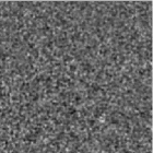
c	d

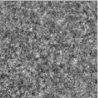
Fig. 2: Images collected by the CCD using the SINF technique (panels a and c) and their power spectra $S\left(Q\right)$ (panels b and d). Data taken at $\vartheta=0$ for two different exposure times: $\Delta t=48\mathrm{ms}$ for panels a and b; $\Delta t=497\mathrm{ms}$ for panels c and d. Data for PTFE dispersion, 0.25% volume fraction in water.

Actually the speckle pattern is not static in time but seems to “boil”, as consequence of the motion of the scattering particles, which generates changes in the beam phase. The image taken at an exposure time $\Delta t=48\mathrm{ms}$ is nearly freezed; on the contrary, the image at $\Delta t=497\mathrm{ms}$ is blurred by the averaging of the speckle motion. Sets of images taken at different exposure times $\Delta t$ contain information on the dynamics of the scattering objects.

The characteristic power spectra $S\left(Q\right)$ of the speckle images are also shown in Fig. 2, where the graphs represent the angular average of the spectra. The image blurring, due to large exposure time, appears as a depression, which is more evident at large wave vectors. Actually, all the information on the dynamics of the image Fourier modes, and hence of the scattered fields, is contained in the ETDS $S\left(Q,\Delta t\right)$, that is, in the image power spectra taken at several different exposure times [17].

Indeed, a set of ETDS, taken at different exposure times, at $\vartheta=0$, is shown in Fig. 3.

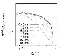
Fig. 3: Exposure time dependent spectra $S^{\vartheta}\left(Q,\Delta t\right)$, measured as functions of the scattering vector $Q$, at two different angles $\vartheta$ between polarizer and analyzer. Left panel: data taken at different exposure time $\Delta t$ with the analyzer at $\vartheta=0$ (VV, polarized component). Right panel: same as left panel, but with analyzer at $\vartheta=82.0^{\circ}$ (VV + VH, sum of polarized and depolarized components). The keys provide the different values of the exposure time $\Delta t$. Data taken for PTFE as in Fig. 2.

The graph on the left refers to the VV component, with $\vartheta=0$. It can be noticed that, as $\Delta t$ increases, the power spectra $S^{\vartheta=0}\left(Q,\Delta t\right)$ taken at $\vartheta=0$ decrease. Moreover, the decrease is stronger at large wave vectors. This can be qualitatively interpreted as a consequence of the translational diffusion of the colloidal particles: light scattered at the transferred wave vector $Q$ has a characteristic time $\tau_{VV}$, decreasing as $Q$ increases, see Eq. (3). For large $Q$ values, the corresponding Fourier modes oscillate faster, and hence the averaging cancels them at shorter exposure times. The graph on the right in Fig. 3 refers to data measured at nearly crossed polarizers, namely $\vartheta=82.0^{\circ}$. As apparent from the graph, as the exposure time $\Delta t$ increases, the ETDS decreases approximately at the same rate for all wave vector. This fact is explained if we recall that the power spectra $S^{\vartheta=82.0^{\circ}}\left(Q,\Delta t\right)$ mainly reflects the VH scattering dynamics. For small wave vectors $Q$, $\tau_{VH}$ scales with the rotational diffusion of the anisotropic colloidal particles, thus being basically constant, see Eq. (4).

Figure 4 shows graphs of the ETDS as a function of the exposure time $\Delta t$, at two fixed $Q$ vectors: $Q=1.23\cdot 10^{6}\mathrm{m}^{-1}$ and $4.42\cdot 10^{6}\mathrm{m}^{-1}$, for two different angles between the polarizer and the analyzer $\vartheta=0$ and $\vartheta=82.0^{\circ}$.

Fig. 4: Exposure-time dependent spectra $S\left(Q,\Delta t\right)$, measured as functions of the exposure time $\Delta t$, at two different angles $\vartheta$ between polarizer and analyzer. Squares: $Q=1.23\cdot 10^{6}\mathrm{m}^{-1}$; dots: $Q=4.42\cdot 10^{6}\mathrm{m}^{-1}$. Filled symbols: $\vartheta=0$; open symbols: $\vartheta=82.0^{\circ}$. The lines represent the fitting curves obtained according to Eq. (17), see text for details. Fitting parameters at $Q=1.23\cdot 10^{6}\mathrm{m}^{-1}$, $\tau_{VV}=0.5\mathrm{s}$ and $\tau_{VH}=6.2\mathrm{ms}$; at $Q=4.42\cdot 10^{6}\mathrm{m}^{-1}$, $\tau_{VV}=36\mathrm{ms}$ and $\tau_{VH}=5.5\mathrm{ms}$. Data taken for PTFE as in Fig. 2.

The data in Fig. 4 are obtained from the data in Fig. 3, and reflect the different blurring of the images at two values of $\vartheta$ and two values of $Q$. It is apparent that the four curves show four different decay behaviors. At small $Q$ the $S\left(Q,\Delta t\right)$ is larger than at large $Q$. Moreover, the scattering at nearly crossed polarizers ($\vartheta=82.0^{\circ}$) approximates the $\vartheta=0$ scattering at large exposure times. This is due to the fact that the rotational time constant is always smaller than the translational one.

6 PTFE discussion

In this section we give a quantitative assessment of the effect of the analyzer on the power spectra $S\left(Q\right)$ of PTFE colloidal particles. We consider the image field as the superposition of three fields: $E_{0}$, the transmitted beam, and the scattered fields $E_{VV}$ and $E_{VH}$, parallel and perpendicular to $E_{0}$:

$${\bf E}={\bf E}_{0}+{\bf E}_{VV}+{\bf E}_{VH}$$ (10)

Beyond the analyzer, the field is:

$$E=E_{0}\cos\vartheta+E_{VV}\cos\vartheta+E_{VH}\sin\vartheta$$ (11)

The intensity is thus proportional to:

$$I=\left|E\right|^{2}\propto\left|E_{0}\right|^{2}+\Re\left[E_{VV}E_{0}^{*}\right]+\Re\left[E_{VH}E_{0}^{*}\right]\tan\vartheta$$ (12)

where $\Re$ is the real part and ^∗ is the complex conjugate and the terms $E_{VV}^{2}$ and $E_{VH}^{2}$ can be neglected because we consider the transmitted beam much stronger than scattered ones (heterodyne condition). All the data processing is performed after normalization of the images’ intensities at a given average intensity. Changing $\vartheta$ modifies only the relative amplitude of the VH contribution to the image, while the VV term is left constant. For our samples, which scatter almost isotropically, the cross correlations between $E_{VV}$ and $E_{VH}$ are negligible. Hence the power spectra is the sum of the VV and VH power spectra:

$$S^{\vartheta}\left(Q,\Delta t\right)=S^{VV}\left(Q,\Delta t\right)+S^{VH}\left(Q,\Delta t\right)\tan^{2}\vartheta$$ (13)

At $\vartheta=0$, we measure the VV signal only:

$$S^{VV}\left(Q,\Delta t\right)=S^{\vartheta=0}\left(Q,\Delta t\right)$$ (14)

Increasing $\vartheta$, we get a mixture of VV and VH components. It can be noticed that the relative intensity of the VV component with respect to the transmitted beam is left unchanged by modifying the analyzer position, and it always contributes to the SINF signal by the same amount. As $\vartheta$ approaches $90^{\circ}$, the relative amplitude of the VH component of the EDTS increases. However, arbitrarily large values cannot be reached, because of the existence of a limit angle, above which the heterodyne condition is violated.

As shown in Fig. 4, rotating the analyzer towards $90^{\circ}$ has the effect of increasing the measured ETDS values. The increment, that is the difference between the ETDS at $\vartheta=82.0^{\circ}$ and $\vartheta=0$, is proportional to the depolarized (VH) ETDS:

$$S^{VH}\left(Q,\Delta t\right)\propto S^{\vartheta=82}\left(Q,\Delta t\right)-S^{\vartheta=0}\left(Q,\Delta t\right)$$ (15)

It has been shown that the relation between $C_{E}\left(Q,t\right)$ and the ETDS $S(Q,\Delta t)$ is [17]:

$$S\left(Q,\Delta t\right)\propto\frac{2}{\Delta t^{2}}\int_{0}^{\Delta t}\mathrm{d}s\left(\Delta t-s\right)C_{E}\left(Q,s\right)$$ (16)

This relation allows us to interpret the ETDS data and to compare them with the results of the dynamic SIFF measurements. For the case of an exponential decay $C_{E}\left(q,t\right)\propto exp\left[-t/\tau\right]$, we have [16, 18, 17]:

$$S\left(Q,\Delta t\right)\propto f\left(\frac{\Delta t}{\tau}\right)$$ (17)

where:

$$f\left(x\right)=\frac{2}{x^{2}}\left(e^{-x}-1+x\right)$$ (18)

Indeed, the ETDS for $\vartheta=0$ in Fig. 4 can be nicely fitted with Eq. (17) with $\tau_{VV}$ as fitting parameter (see filled symbols in Fig. 4 and the fitting curves).

The VH ETDS has been obtained by Eq. (15) and has been fitted with Eq. (17), with $\tau_{VH}$ as fitting parameter. The obtained values are then used in the ETDS at $\vartheta=82.0^{\circ}$, shown in Fig. 4 (see open symbols and their fitting curves). It is worth noting that, given its rotational diffusive behavior, the VH component has a constant characteristic decay time, for both wave vectors $Q$ (see Eq. (4) ). By contrast, the VV component shows a faster decay at larger wave vectors $Q$, reflecting its translational diffusive behavior (see Eq. (3)).

The values of $\tau_{VV}$ and $\tau_{VH}$, obtained by the fitting procedure described above, are shown for several wave vectors $Q$ in Fig. 5.

Fig. 5: Decay times $\tau_{VV}$ and $\tau_{VH}$, obtained by the described fitting procedure, and plotted as functions of the scattering wave vector $Q$. Lines represent a fitting on $\tau_{VV}$ and $\tau_{VH}$ with Eq. (3) and Eq. (4). Values obtained by the fit $D_{T}=1.4\cdot 10^{-12}\mathrm{m}^{2}/\mathrm{s}$ and $\Theta=23.8\mathrm{s}^{-1}$. Data taken for PTFE as in Fig. 2.

At the end, by fitting the resulting data with Eq. (3) and Eq. (4), the translational and rotational diffusion coefficients of the sample are obtained. The outcomes of this fitting procedure for PTFE sample are $D_{T}=1.4\cdot 10^{-12}\mathrm{m}^{2}/\mathrm{s}$; $\Theta=23.8\mathrm{s}^{-1}$, in very good agreement with the values obtained with the traditional dynamic SIFF apparatus.

7 DR1 experimental results and discussion

The analysis and the discussion of depolarized SINF measurements for the DR1 sample follows the one used for PTFE. Namely, we collect the images with parallel and nearly crossed polarizer/analyzer, and then we calculate the power spectra $S\left(q,\Delta t\right)$ at different exposure times $\Delta t$.

The $\vartheta=0$ ETDS $S^{VV}\left(q,\Delta t\right)$ are simply fitted with Eq. (17). The characteristic times $\tau_{VV}$ obtained with the fitting procedure are shown in Fig. 6.

Fig. 6: Decay times and fitting lines as for Fig. 5. Values obtained by the fit: $D_{T}=2.3\cdot 10^{-12}\mathrm{m}^{2}/\mathrm{s}$; $\Theta=28.2\mathrm{s}^{-1}$, $\alpha=0.477$. Data taken for the DR1 sample in water, at 1% volume fraction.

The VH component is evaluated using Eq. (15). In this case the analysis is somewhat different, because the field autocorrelation function is the stretched exponential described by Eq. (7). The ETDS can be calculated through Eq. (16), and the outcome is:

$$S^{VH}\left(Q,\Delta t\right)\propto f_{\alpha}\left(\frac{\Delta t}{\tau_{VH}}\right)$$ (19)

where:

$$f_{\alpha}\left(x\right)=\frac{2}{\alpha x}\left[\gamma\left(\frac{1}{\alpha},x^{\alpha}\right)-\frac{1}{x}\gamma\left(\frac{2}{\alpha},x^{\alpha}\right)\right],$$ (20)

and $\gamma\left(a,x\right)$ is the lower incomplete gamma function:

$$\gamma\left(a,x\right)=\int^{x}_{0}e^{-t}t^{a-1}\mathrm{d}t$$ (21)

For $\alpha=1$, the function $f_{\alpha}\left(x\right)$ reduces to the already described $f\left(x\right)$ shown in Eq. (18).

The characteristic times $\tau_{VH}$, obtained by fitting $S^{VH}\left(Q,\Delta t\right)$ with Eq. (19), are shown in Fig. 6.

From the VV term, we get $D_{T}=2.3\cdot 10^{-12}\mathrm{m}^{/}\mathrm{s}$. From the VH term, we get $\Theta=28.2\mathrm{s}^{-1}$; $\alpha=0.477$. All the SINF fitting results are very close to the SIFF results.

Figure 7 shows the comparison between the VH intensity autocorrelation function measured with SIFF, and the VH ETDS measured with SINF, evaluated with Eq. (15).

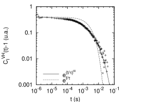
Fig. 7: Left panel: depolarized VH intensity autocorrelation function $C_{I}^{VH}\left(t\right)$ measured as a function of delay time $t$, by using traditional SIFF apparatus, at $Q=2.5\cdot 10^{6}\mathrm{m}^{-1}$. The lines represent a fit with a stretched exponential or a single exponential decay. Fitting parameters: $\Theta=27.8\mathrm{s}^{-1}$; $\alpha=0.523$. Right panel: depolarized VH ETDS measured as a function of exposure time $\Delta t$, by using SINF apparatus, at $Q=2.1\cdot 10^{6}\mathrm{m}^{-1}$. The lines represent a fit with $f_{\alpha}\left(x\right)$ from Eq. (20) (which is related to a stretched exponential), or a fit with $f\left(x\right)$ from Eq. (18) (which is related to a single exponential). Fitting parameters: $\Theta=28.2\mathrm{s}^{-1}$, $\alpha=0.477$. Data taken for DR1 sample as in Fig. 6.

As it appears from the figure, the stretched exponential decay is clearly demonstrated by both techniques.

8 Conclusions

In this paper we present original data obtained with a polarized and depolarized SINF instrument, here described for the first time. By using the proposed technique, the translational and rotational diffusion coefficients of generic rod-like colloidal particles can be measured. The procedure has been validated with PTFE and iron oxide rod-like colloidal samples. The obtained diffusion coefficients of the rods are in very good agreement with the data acquired with a traditional dynamic SIFF apparatus. The proposed method allows a simultaneous measurement of the diffusion coefficients on a very large wave vector range, opening the way to detailed studies of passive and active motions in anisotropic colloidal systems, ranging from nanoparticles to biological entities such as viruses, bacteria, proteins, and macromolecules.