Negativity of the Coarse Grained Wigner Function as a Measure of Quantal Behavior

Abstract

The negativity of a given state’s Wigner function has been proposed as a measure of quantumness of that state in a unipartite system. This otherwise physically intuitive and useful phase-space measure however does not yield the right correspondence principle limit, and also turns out to yield infinite values of the infinite square well. We show that both these issues can be sensibly resolved using coarse-graining of the Wigner function.

I Introduction

A numerical measure of the “quantumness” of a system is useful in many contexts, for example in nonlinear optics or studies of the transition from quantum-to-classical behavior. There are various ways of parameterizing nonclassicality. It is typical to start by defining a quantum coherent state with minimum uncertainty as the most classical system possible, then measuring how different the system in question is from such a coherent state. The difference between these two states is often quantified by finding the minimum distance between them based on the trace, the Hilbert-Schmidt distance, or some other similar metricdodonov . Alternatively, the distance between a given system and the closest classical system can be measured using the Cahill parameter $\tau$. The minimum value of $\tau$ which produces a positive definite distribution function can be interpreted as the ”nonclassical depth” of the system, which in turn may be used as an index of quantumnesslee . A more thorough discussion of many of the nonclassicality parameters that have been studied can be found in Dodonovdodonov .

Recently, it has been arguedkenfack that the negativity of a given state’s Wigner function is a simple and clean measure of that state’s quantumness. One advantage of this method is that the Wigner representation can be determined experimentallyroyer , as well as the fact that the negativity is a measure of non-locality for bi-partite or multi-partite systems. Further, for a unipartite system, this is an intuitive measure. Since Wigner functions are quasi-probabilities existing in phase-space, they are directly comparable with classical probability functions, and this is often done in understanding quantum-classical correspondence issues, for example. There is no negativity in classical probablities, of course. The negativity, or negative volume, of a Wigner function $W(x,p)$ defined as:

$$\eta=\int_{-\infty}^{\infty}\int_{-\infty}^{\infty}\frac{\left|W(x,p)\right|-W(x,p)}{2}dxdp$$ (1)

Since the parts of the Wigner function that are negative decrease as the system decoheres under the influence of an environment, this further reinforces the notion that the Wigner function’s negativity is a useful measure.

In the case of the one-dimensional harmonic oscillator, $\eta$ increases approximately as $\sqrt{n}$ when measured for eigenstates of different $n$kenfack . At low values of $n$, this is sensible – we expect that the increased oscillations as we climb the eigenfunction ladder do indeed correspond to greater quantumness. However, this does not hold at high values of $n$. The correspondence principle dictates that the limit as $n\rightarrow\infty$ of the harmonic oscillatorsegatto should yield a transition from quantum to classical behavior. As such, a monotonic increase in quantumness with $n$ is not correct. Moreover, simple intuition runs counter to the possibility that any system becomes extremely quantum at the high energies associated with the macroscopic world; even if the quantumness of such a system did not drop off to zero at high $n$, its higher energy states should at the very least not be orders of magnitude more quantum than the lower states where quantum behavior is usually observed.

As a way of dealing with this counter-intuitive aspect of the otherwise sensible measure, we propose ‘coarse-graining’ the Wigner function by convolving it with a Gaussian before measuring its negativity as

$$\eta =\int_{-\infty}^{\infty}\int_{-\infty}^{\infty}\frac{\left|W_{CG}(x,p)\right|-W_{CG}(x,p)}{2}dxdp,$$ (2)

$$\text{where }W_{CG}(x,p) =\int_{-\infty}^{\infty}\int_{-\infty}^{\infty}\exp[-\delta((x-x^{\prime})^{2}+(p-p^{\prime})^{2})]W(x^{\prime},p^{\prime})dx^{\prime}dp^{\prime}.$$ (3)

Mathematically, convolution with a Gaussian has the effect of smoothing out the Wigner function, reducing the magnitude of local oscillations. This physically motivated technique that has often been used to study semiclassical behavior in quantum systems. Coarse-graining has the effect of smoothing away small and purely quantum features while maintaining the large-scale structure from which classical behavior typically emergesrivas . As discussion in the literature showshabib ; wilkie , coarse-graining is necessary to retrieve classical behavior from some quantum systems. It represents the reality that quantum-classical correspondence for closed quantum systems provides a singular classical limit – by this we mean that $\hbar=0$ can be qualitatively, not just quantitatively, different from any non-zero value of $\hbar$. If the negativity of the Wigner function is to be a meaningful measure of the classicality of such systems, it is an intuitive step to include coarse-graining. In fact, as we show below, this procedure indeed resolves the paradoxical behavior(s) of the negativity.

Moreover, as we show below, the infinite square well, another textbook example, also benefits from this procedure. Without coarse-graining, eigenfunctions of this system have infinite negativity, which again renders this otherwise useful measure less useful, but coarse-graining renders the negativity finite.

In what follows, we present our results for the harmonic oscillator, followed by the infinite square well, and conclude with a short discussion.

II The Harmonic Oscillator

In arbitrary units where $m=\omega=\hbar=1$, the Wigner function for the $n^{th}$ eigenstate of a quantum harmonic oscillator iskenfack

$$W_{n}(x,p)=2\frac{(-1)^{n}}{\pi}\exp[-2(x^{2}+p^{2})]L_{n}[4(x^{2}+p^{2})]$$ (4)

where $L_{n}$ denotes the $n^{th}$ Laguerre polynomial. After coarse-graining this function as in Eq. (2), if $\delta$ is an integer, the resulting function takes the form

$$W_{CG,n}(x,p)=ke^{\frac{2n}{\delta+2}(x^{2}+p^{2})}P_{n}(x,p)$$ (5)

where $k$ is an arbitrary numerical constant, and $P_{n}(x,p)$ is an $n^{th}$ order polynomial function of $(x^{2}+p^{2})$. For example we have that

$$W_{\delta=3,n=4}=6.84\times 10^{-2}e^{-\frac{6}{5}(x^{2}+p^{2})}[(x^{2}+p^{2})^{4}-\frac{20}{9}(x^{2}+p^{2})^{3}+\frac{25}{18}(x^{2}+p^{2})^{2}-\frac{125}{486}(x^{2}+p^{2})+\frac{625}{69984}]$$

$$W_{\delta=5,n=2}=0.947\times e^{-\frac{10}{7}(x^{2}+p^{2})}[(x^{2}+p^{2})^{2}-\frac{21}{25}(x^{2}+p^{2})+\frac{441}{5000}]$$

For the special case $\delta=2$, which corresponds to $\Delta x\Delta p=\frac{\hbar}{2}$, this reduces to

$$W_{CG,2}(x,p)=\frac{1}{2n!}e^{-(x^{2}+p^{2})}(x^{2}+p^{2})^{n}$$ (6)

which looks like a classical orbit. This function is positive definite, meaning that, as expectedsoto , no quantumness can be observed with blurring greater than or equal to minimum uncertainty. The Husimi function, a positive-definite quantum ‘probability’ function in phase-space is, in fact, constructed by coarse-graining the Wigner function with a minimum-uncertainty Gaussian. This result implies that in this specific case the ‘least’ amount of coarse-graining needed to get a function indistinguishable from classical is precisely the Husimi coarse-graining. Since the harmonic oscillator basis can be used to construct an arbitrary state, this means that a general state becomes positive definite if and only if a Husimi coarse-graining is used.

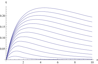
Figure 1: Negativity $\eta$ of the harmonic oscillator’s smoothed Wigner function at various $n$ shown for $\delta$’s increasing from 3 on the bottom to 14 on top. As $\delta$ increases, the peak in negativity moves to higher $n$.

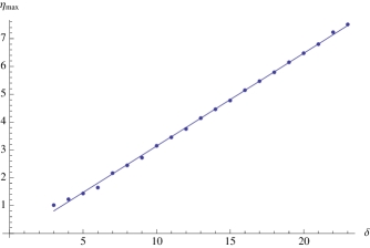
Figure 2: The eigenfunction with maximum negativity $n_{max}$ increases monotonically and roughly linearly as a function of $\delta$.

More interestingly, once the Wigner function is coarse-grained, its negativity no longer increases monotonically with $n$, and regardless of $\delta$, negativity does not decrease monotonically with $n$ either. Rather, negativity increases sharply to some $n_{max}$, then tapers off to approach zero as $n\rightarrow\infty$ (Fig. 1). As $\delta$ increases, so does the $n$ value at which maximum negativity is observed. All of these properties are satisfyingly in line with physical intuition and provide a post facto justification for the coarse-graining procedure. The relationship between $\delta$ and $n_{max}$ seems to be roughly linear, as can be seen in Fig. (2). More specifically, the relation between $\eta_{max}$ and $\delta$ is best fit by a line with slope $\approx\frac{1}{3}$ for which we have no qualitative explanation.

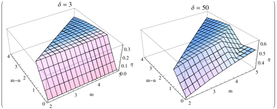
Figure 3: Negativity $\eta$ of the harmonic oscillator’s smoothed Wigner function for the state $\left|m\right\rangle\left\langle n\right|$ shown as a function of $m$ and $m-n$ in both the $\delta=3$ and $\delta=50$ cases.

In addition to the Wigner function for the $n^{th}$ eigenfunction, an arbitrary state for the harmonic oscillator will have a Wigner function with “off-diagonal” elements arising from the combination of two or more pure states. For instance, for a harmonic oscillator state $\left|\psi\right\rangle=\left|m\right\rangle+\left|n\right\rangle$, the overall wave function $\left|\psi\right\rangle\left\langle\psi\right|$ could be written as $\left|m\right\rangle\left\langle m\right|+\left|n\right\rangle\left\langle n\right|+\left|m\right\rangle\left\langle n\right|+\left|n\right\rangle\left\langle m\right|$, with $\left|m\right\rangle\left\langle n\right|$ and $\left|n\right\rangle\left\langle m\right|$ being the off-diagonal elements. In the same arbitrary units as above where $m=\omega=\hbar=1$, the Wigner functions of these off-diagonal elements are given bygarraway

$$W_{m,n}(x,p)= 2\frac{(-1)^{n}}{\pi}\sqrt{\frac{n!}{m!}}\exp[-2(x^{2}+p^{2})](2\sqrt{x^{2}+p^{2}})^{m-n}*$$

$$\cos((m-n)\arctan(\frac{p}{x}))L_{n}^{m-n}[4(x^{2}+p^{2})]$$ (7)

Some of the negativities for various combinations of $n$ and $m$ at a few different values of $\delta$ are shown in Fig. 3. The complexity of equation II makes a thorough analysis of the behavior of smoothed, off-diagonal Wigner functions computationally difficult. Nevertheless, a few features of Fig. 3 are worth pointing out. All values of $m-n$ show the same basic pattern of increasing negativity with increasing $m$, at least up to a point. It is also interesting that the $m-n=0$ cases (i.e. the on-diagonal elements) tend to have significantly lower negativities than any other values of $m-n$. This is commensurate with intuition that a superposition of quantum states is in some sense a more non-classical state. Irrespective the existence of any patterns, it is important to note that the off-diagonal Wigner functions can in principle be analytically coarse-grained. Since the harmonic oscillator states form a basis for all infinite states, any infinite Wigner function can then be expressed as a superposition of on- and off-diagonal square well states, and therefore sensibly coarse-grained analytically before measuring its negativity.

III The Square Well

The infinite square well provides another case in which coarse-graining before calculating negativity is a useful tool. The Wigner function for the $n$th eigenstate of an infinite square well of width $\pi$ isbelloni

$$W(x,p)=\frac{2}{\pi^{2}\hbar}(\frac{\sin[2(p/\hbar+n)x]}{4(p/\hbar+n)}+\frac{\sin[2(p/\hbar-n)x]}{4(p/\hbar-n)}-\cos(2nx)\frac{\sin[2px/\hbar]}{2p/\hbar})$$ (8)

where $x\in[0,\pi/2]$; for $x\in[\pi/2,\pi]$, the expression is identical, except all occurences of $x$ are replaced by $L-x$. A particle in the infinite well can only occupy a finite range of positions but can have any momentum, so the support of this Wigner function covers $x\in[0,\pi]$ and $p\in[-\infty,\infty]$.

That the negativity of this function is infinite is demonstrated by starting from the observation that the integral of negativity over $p$ from $-\infty$ to $\infty$ will diverge if the integral from any $p_{0}$ to $\infty$ diverges. To simplify calculations in the following analysis of divergence, we will examine some $p_{0}>>\hbar n$ so that the $nx$ terms in equation (8) become negligible. The integral computing the negativity between $p_{0}$ and $\infty$ then becomes:

$$\frac{1}{\pi^{2}}\int_{p_{0}}^{\infty}\bigg{(}\int_{0}^{\pi/2}\mathbf{Neg}[(1-\cos[2nx])\frac{\sin[2(p/\hbar)x]}{p}]dx+$$

$$\int_{\pi/2}^{\pi}\mathbf{Neg}[(1-\cos[2n(\pi-x)])\frac{\sin[2(p/\hbar)(\pi-x)]}{p}]dx\bigg{)}dp$$ (9)

where

$$\mathbf{Neg}[x]=\begin{cases}-x&\text{if $x<0$,}\\ 0&\text{if $x\geq 0$.}\end{cases}$$

A variable substitution in the second line of equation (III) further reduces it to:

$$\frac{2}{\pi^{2}}\int_{p_{0}}^{\infty}\int_{0}^{\pi/2}\mathbf{Neg}[(1-\cos[2nx])\frac{\sin[2px/\hbar]}{p}]dxdp.$$ (10)

Since $(1-\cos[2nx])$ and $\frac{1}{p}$ will both always be positive over the domain of integration, they can be pulled out of the Neg operator, leaving the equation in the form

$$\frac{2}{\pi^{2}}\int_{p_{0}}^{\infty}\int_{0}^{\pi/2}(1-\cos[2nx])\frac{{\bf Neg}[\sin[2px/\hbar]]}{p}dxdp.$$ (11)

The average value of Neg$[\sin[2px/\hbar]]$ over a single period of oscillation is $\frac{1}{\pi}$. As $p\rightarrow\infty$, the period of oscillation $\rightarrow$ 0, so Neg$[\sin[2px/\hbar]]$ effectively becomes a constant multiplier of $\frac{1}{\pi}$ in the large-$p$ limit, yielding the integral

$$\frac{2}{\pi^{3}}\int_{p_{0}}^{\infty}\int_{0}^{\pi/2}(1-\cos[2nx])\frac{1}{p}dxdp=\frac{1}{\pi^{2}}\int_{p_{0}}^{\infty}\frac{dp}{p}$$ (12)

which is divergent.

It is certainly interesting that the negativity of this Wigner function is divergent, especially since the Wigner function itself is defined to be normalized. The fact that the infinite square well’s negativity diverges while the harmonic oscillator’s does not points at a fundamental difference between the two systems, and merits further consideration. Nevertheless, the divergence of equation (12) makes unsmoothed negativity an unhelpful metric when dealing with square wells or any states in a finite position-space domain, since those can always be expressed as a superposition of square well states.

Coarse-graining the Wigner function before measuring negativity provides a solution to this difficulty. We can demonstrate this with the following argument: Since the Wigner function (smoothed or not) is by definition finite and continuous, we need not worry about divergence of the negativity integral except over infinite regions. Moreover, since equation (8) is symmetric in $p$, the integral of negativity over all phase space will converge if the integral from $0\text{ to }\infty$ converges. Combining these two observations, we can see that when proving the convergence of negativity over the entire Wigner function, it is sufficient to show convergence from any $p_{0}\text{ to }\infty$. Here as before, we examine some $p_{0}>>\hbar n$ to simplify calculations. By applying the same steps to the smoothed Wigner function that we applied to the unsmoothed Wigner function in reaching equation (10), we obtain the expression:

$$\frac{2}{\pi^{2}}\int_{p_{0}}^{\infty}\int_{0}^{\pi}\mathbf{Neg}[\int_{p_{0}}^{\infty}\int_{0}^{\pi}{}e^{-\delta((x-x^{\prime})^{2}+(p-p^{\prime})^{2})}(1-\cos[2nx^{\prime}])\frac{\sin[2p^{\prime}x^{\prime}/\hbar]}{p^{\prime}}dx^{\prime}dp^{\prime}]dxdp$$ (13)

which can be rewritten as

$$\frac{2}{\pi^{2}}\int_{p_{0}}^{\infty}\int_{0}^{\pi}\mathbf{Neg}[\int_{p_{0}}^{\infty}\frac{1}{p^{\prime}}e^{-\delta(p-p^{\prime})^{2}}F(p^{\prime},x)dp^{\prime}]dxdp$$ (14)

$$\text{where }F(p^{\prime},x)=\int_{0}^{\pi}{}e^{-\delta(x-x^{\prime})^{2}}(1-\cos[2nx^{\prime}])\sin[2p^{\prime}x^{\prime}/\hbar]dx^{\prime}$$

Based on numerical analysis with Mathematica, $F(p^{\prime},x)$ is an oscillating function of $p^{\prime}$ with an amplitude that decreases as $\frac{1}{p^{\prime}}$ for sufficiently large $p^{\prime}$. Since the negative value of this function will always be $\leq\frac{k}{p^{\prime}}$, where $k$ is some constant dependent on $x$ and $\delta$, Eq. (14) must have a value less than or equal to:

$$\frac{2}{\pi^{2}}\int_{p_{0}}^{\infty}\int_{0}^{\pi}\mathbf{Neg}[\int_{p_{0}}^{\infty}-\frac{k}{p^{\prime 2}}e^{-\delta(p-p^{\prime})^{2}}dp^{\prime}]dxdp$$ (15)

Furthermore, after convolution with a Gaussian in $p$, the function $\frac{k}{p^{2}}$ still drops off as some constant over $p^{2}$, so Eq. (15) further reduces to:

$$\frac{1}{\pi^{2}}\int_{p_{0}}^{\infty}\int_{0}^{\pi}\frac{k}{p^{2}}dxdp$$ (16)

which clearly converges. Since the value of this integral is greater than or equal to the integral of negativity from $p_{0}\text{ to }\infty$, this integral must converge. Thus, the integral of negativity over all phase space must converge. Note that this proof is independent of $\delta$; any degree of coarse-graining will allow the integral to converge.

Some of the coarse-grained negativities of an infinite square well of length $\pi$ are shown in Fig. 4. For any $\delta$, negativity generally increases with increasing $n$ over the range shown. However, this growth is not monotonic; at $n=8$, negativity decreases slightly from $n=7$. It is also worth noting that the negativities for $n=5\text{ and }n=6$ seem to show a strong dependence on $\delta$ that is absent from the rest of the graph. The significance of these features is at present unclear. They may correspond with actual variations in a square well’s properties at different energy levels, or they may simply indicate that small fluctuations in $\eta$ should be ignored when considering larger trends in a system’s Wigner function. In either case, comparisons of calculated negativities with experimental square well behavior will be needed to determine how much of a fluctuation in $\eta$ constitutes a significant physical change. Note also that the coarse-grained Wigner function becomes positive definite for $\delta=1$, which, in the units used for this problem, corresponds to the minimum uncertainty Gaussian again.

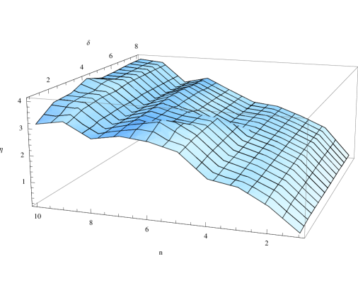
Figure 4: The negativity $\eta$ of an infinite square well’s smoothed Wigner function at various $n$ and $\delta$. Negativity seems to increase, albeit non-monotonically, with $n$ for all $\delta$.

IV Discussion

While it is satisfying to see that coarse-graining the Wigner function before computing its negativity resolves some critical issue with this measure of quantumness, it invites the question of the physical interpretation of $\delta$. That is, what determines the degree of theoretical coarse-graining applied to a given Wigner function? One obvious consideration is that $\delta$ should be understood as a measure of the amount of thermal noise present that is affecting the system, whence the coarse-graining represents the ‘washing out’ of small quantum features by thermal fluctuations. Under this interpretation, the increase in $n_{max}$ with increasing $\delta$ would correspond to the fact that larger systems can exhibit quantum behavior at sufficiently low temperatures, as is intuitive, while still providing for an appropriate ’correspondence principle’ behavior for sufficiently high $n$.

Alternatively, $\delta$ could be based on the precision of whatever measurements are being taken on the system. In this case, $\eta$ would be less an index of the quantumness present in a system and more an index of how much of a system’s quantumness could be observed given a certain precision of measurement. This interpretation could be useful in examining the classical-to-quantum transition as one ’zooms out’ from the Planck scale and sacrifices small-scale precision for a more macroscopic view. It could also be useful in searching for macroscopic quantum behavior: Systems showing high negativity even after strong coarse-graining might be expected to show quantum behavior even on large scales.

References

- (1) V. V. Dodonov, O. V. Man’ko, V. I. Man’ko, P. N. Lebedev, and A. Wunsche. J. Mod. Opt., 47, 633 (2000).
- (2) C.T. Lee. Phys. Rev. A44, 2775 (1991).
- (3) A. Kenfack and K. Zyczkowski J. Opt. B: Quantum Semiclass. Opt.6 396 (2004).
- (4) A. Royer. Phys. Rev. Lett. 55, 2745 (1985).
- (5) B. R. Segatto, J. C. S. Azevedo, and M. M. de Souza. J.Phys.A,36 5115 (2003).
- (6) A. M. F. Rivas, E. G. Vergini, and D. A. Wisniacki. Eur. Phys. Jour. D 32, 355 (2005).
- (7) S. Habib and R. Laflamme. Phys. Rev. D42, 4056 (1990).
- (8) J. Wilkie and P. Brumer, Phys. Rev. A55, 27 (1997); ibid 55, 43 (1997).
- (9) F. Soto and P. Claverie. Physica A, 109, 193 (1981).
- (10) B. M. Garraway and P. L. Knight. Phys. Rev. A46 5346 (1992).
- (11) M. Belloni, M. A. Doncheski, and R. W. Robinett. Am. J. Phys. 72, 1183 (2004).