Quantitative complementarity between local and nonlocal character of quantum states in a three-qubit system

Abstract

Local or nonlocal character of quantum states can be quantified and is subject to various bounds that can be formulated as complementarity relations. Here, we investigate the local vs. nonlocal character of pure three-qubit states by a four-way interferometer. The complete entanglement in the system can be measured as the entanglement of a specific qubit with the subsystem consisting of the other two qubits. The quantitative complementarity relations are verified experimentally in an NMR quantum information processor.

I Introduction

Classical physics groups physical entities in categories that are considered to be mutually exclusive, such as waves and particles. However, many experimental results are incompatible with this approach, since they can not be explained in terms of a pure wave picture or a pure particle picture. Quantum mechanics was developed to resolve this discrepancy and Bohr introduced the concept of complementarityBohr (1928) to emphasize the different approach. The most familiar aspect of complementarity is perhaps the wave-particle duality. It means, e.g., that light has characteristic properties that are usually associated with particles but also show behavior usually associated with waves. If we design an experiment to measure any of these properties, it can only be achieved at the cost of losing information about the other.

Complementarity is often illustrated by means of a two-way interferometer such as Young’s double-slit experiment or a Mach-Zehnder setup. Already in 1909, the interference pattern of “single photons” was observed experimentally in a double-slit interference experiment by TaylorTaylor (1909) and later by Dempster and Batho Dempster and Batho (1927). This was of course possible only because these experiments did not provide any information about the path taken by the photons in the double-slit interferometer. The same effect was also observed with many other kinds of single quantum objects including electrons Moellenstedt and Joensson (1959); Tonomura et al. (1989), neutrons Zeilinger et al. (1988), trapped ions Eichmann et al. (1993), atoms Carnal and Mlynek (1991), and even molecules Arndt et al. (1999).

At the qualitative level, complementarity is thus a well established concept. More recently, it was found that complementarity can be quantified Wootters and Zurek (1979); Bartell (1980); Greenberger and Yasin (1988); Mandel (1991); Jaeger et al. (1995); Englert (1996); Englert and Bergou (2000). For the case of the wave-particle complementarity, it is possible to formulate it in terms of the inequality

$$P^{2}+V^{2}\leq 1.$$ (1)

In this expression, the particle-like property is quantified by the predictability $P$, which specifies a priori knowledge of the path that the system will follow (“which-way”information), whereas the wave-like properties are quantified by the visibility $V$ of the interference fringes. In the case of a pure quantum state, the inequality turns into the limiting equality. While this wave-particle duality was considered mostly in two-path interferometers, it is possible to generalize it to multi-path interferometers Englert et al. (2007).

Quantitative complementarity relations exist not only for individual quantum systems, but even more for composite systems. In systems consisting of two quantons, some new complementarity relations were found, such as the complementarity relation between single and two-particle fringe visibilitiesJaeger et al. (1993, 1995), between distinguishability and visibilityEnglert (1996), and between the coherence and predictabilityEnglert and Bergou (2000) in a quantum eraserScully and Zubairy (1997). These properties are less directly measurable, but some can be quantified, e.g. by two-particle interferometry. Many of these complementarity relations have been experimentally investigated by interferometric experiments, using a wide range of composite two-quanton systems including photons Scully et al. (1991); Schwindt et al. (1999); Kim et al. (2000); Abouraddy et al. (2001); Pryde et al. (2004), atomsDürr et al. (1998a, b) and nuclear spins in a bulk ensemblePeng et al. (2003, 2005); Zhu et al. (2001).

In the course of the study of complementarity in composite systems, entanglement is found to be a key entry. As a purely quantum correlation with no classical counterpart, entanglement can be used to quantify the non-local aspects of the composite system. Some progress has been achieved in this direction, such as the complementarity relations between distinguishability and entanglementOppenheim et al. (2003), between spatial coherence of biphoton wave functions and entanglement Saleh et al. (2000), between local and nonlocal information Bose and Home (2002), and a beautiful equality between visibility, predictability and entanglement in pure two-qubit statesJakob and Bergou (2003). Additionally, some complementarity relations in n-qubit pure systems were found, such as the relationship between multipartite entanglement and mixedness for special classes of n-qubit systemsJaeger et al. (2003), and between the single particle properties and the n bipartite entanglements in an arbitrary pure state of n qubitsTessier (2005).

In our previous paper Peng et al. (2005), we found a complementarity relation that exists in an n-qubit pure state:

$$C_{k(ij...m)}^{2}+S_{k}^{2}=1.$$ (2)

This relation implies a tradeoff between the local single-particle property ($S_{k}^{2}$) whose two constituents are $P_{k}^{2}$ and $V_{k}^{2}$, and the nonlocal bipartite entanglement between the particle and the remainder of the system ($C_{k(ij...m)}^{2}$), defined in terms of the marginal density operator $\rho_{k}$ Rungta et al. (2001); Rungta and Caves (2003)

$$C_{k(ij...m)}=\sqrt{2\left[1-Tr\left(\rho_{k}^{2}\right)\right]}.$$ (3)

Moreover, a conjecture was made: the bipartite entanglement $C_{k(ij...m)}^{2}$ might be equal to the sum of all possible pure multi-particle entanglement(s) connected to this particle Peng et al. (2005). This conjecture was proved for pure two- and three-qubit systems Peng et al. (2005). Therefore, measuring the bipartite entanglement $C_{k(ij...m)}^{2}$ implies that we obtain an entire entanglement (nonlocal) connected to this particle. Therein the simplest case with two qubits has been verified by NMR interferometry, i.e., $C^{2}+S_{k}^{2}=1$, where $C$ is the concurrence of a two-qubit state $\psi$ which is related to ”the entanglement of formation” Wootters (1998), defined by

$$C(\psi)=|\langle\psi|\sigma_{y}\otimes\sigma_{y}|\psi^{\ast}\rangle|.$$

where $\sigma_{y}$ is the $y$ component of the Pauli operator and $\left|\psi^{\ast}\right\rangle$ is the complex conjugate of $\left|\psi\right\rangle$.

The question that was left open in this earlier paper is, if it is possible to test the complementarity relation in a system with more than two qubits. The present paper shows an example for such an experimental test in a pure three-qubit system. For a pure state $|\xi\rangle$ of a three-qubit system ABC, we use a generalized four-way interferometer to verify the complementarity relation

$$C_{A(BC)}^{2}(|\xi\rangle)+S_{A}^{2}(|\xi\rangle)=1.$$ (4)

This experiment uses a specific property of pure three-qubit states. In the next section, we will describe this property and the experimental configuration used to measure the quantities of Eq (4). Sec. III adds details about the main components (transducers) in the interference experiment. In section IV, we combine the interferometer with state preparation and readout. Section V gives experimental details of the implementation in an NMR quantum information processor for different classes of pure 3-qubit states and discusses the results.

II Experimental setup for a three-qubit system

II.1 Preferred basis

Let us express the pure state $|\xi\rangle$ of the three-qubit system ABC in the standard basis ${|ijk\rangle}$ ($i,j,k=0,1$):

$$|\xi\rangle=\sum_{i,j,k}a_{ijk}|ijk\rangle.$$ (5)

The coefficients $a_{ijk}$ are normalized to 1. If we regard the pair BC as a single object, it makes sense to consider the concurrence $C_{A(BC)}$ between qubit A and the composite object consisting of the two qubits B and C.

An interesting and unique property of a pure state $|\xi\rangle$ of the three-qubit system helps us to design an experimental scheme for measuring the concurrence $C_{A(BC)}$ by an interference experiment: The reduced density matrix $\rho_{BC}$ has at most two nonzero eigenvalues. Accordingly, even though the state space of BC is four dimensional, only two of those dimensions are necessary to express the state $|\xi\rangle$ of ABC Coffman et al. (2000). Therefore, the state $|\xi\rangle$ can always be rewritten as

$$|\xi\rangle=\sum_{i,j=0}^{1}b_{ij}|i\rangle_{A}|\Phi_{j}\rangle_{BC}$$ (6)

where $|\Phi_{i}\rangle$ are the eigenstates with the two nonzero eigenvalues of the reduced density matrix $\rho_{BC}=Tr_{A}(|\xi\rangle\langle\xi|)$, and the real coefficients $b_{ij}$ are normalized to 1. Therefore, we can treat A and BC, at least for the present purpose, as a pair of qubits in a pure state.

Like in a two-qubit system, we can thus design a four-way interferometer for a pure 3-qubit state, which consists of four paths, which we label by the corresponding basis states $\{|0\rangle_{A},|1\rangle_{A},|\Phi_{0}\rangle_{BC},|\Phi_{1}\rangle_{BC}\}$. Figure 1 shows the reference setup: The source S emits three particles A, B and C in a pure state. Particle A can propagate along path $|0\rangle_{A}$ and/or $|1\rangle_{A}$, through a variable phase shifter $\varphi_{1}$. Beamsplitter BS₁ connects the two paths and the particles are then registered in either beam $|K_{1}\rangle_{A}$ or $|L_{1}\rangle_{A}$. One the other side the pair of particles B and C as a whole can propagate along the paths $|\Phi_{0}\rangle_{BC}$ and/or $|\Phi_{1}\rangle_{BC}$. The probabilities of the joint (e.g. $p(|K_{1}\rangle_{A}|K_{2}\rangle_{BC})$) and single (e.g. $p(|K_{1}\rangle_{A})$) events generate interference patterns as a function of the phase angles $\varphi_{i}$, depending on the state $|\xi\rangle$ of the source S.

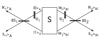
Figure 1: Schematic four-way interferometer in a pure 3-qubit system, using beam splitters BS₁, BS₂ and phase shifters $\varphi_{1}$, $\varphi_{2}$.

From the resulting one-party interference pattern of qubit A, the single-particle fringe visibility is defined as

$$\mathcal{V}_{A}=\frac{\left[p\left(\left|x\right\rangle_{A}\right)\right]_{\max}-\left[p\left(\left|x\right\rangle_{A}\right)\right]_{\min}}{\left[p\left(\left|x\right\rangle_{A}\right)\right]_{\max}+\left[p\left(\left|x\right\rangle_{A}\right)\right]_{\min}},$$ (7)

where $x=K_{1}$ or $L_{1}$, and $p_{min}$ and $p_{max}$ are the minimal and maximal probabilities (as a function of $\varphi_{1}$). The other quantity related to the single-party property of particle A is the predictability $\mathcal{P}_{A}$, which quantifies the a priori which-way knowledge. It is defined as

$$\mathcal{P}_{A}=|\langle\xi|\sigma^{A}_{z}|\xi\rangle|$$ (8)

where $\sigma^{A}_{z}=\left(\begin{array}[]{cc}1&0\\ 0&-1\end{array}\right)$ is the z component of the Pauli oprator. $\mathcal{P}_{A}$ thus measures the magnitude of the probability difference that particle A takes path $|0\rangle$ or the other path $|1\rangle$.

We combine these two single-party properties into a single entity

$$\mathcal{S}^{2}_{A}=\mathcal{V}^{2}_{A}+\mathcal{P}^{2}_{A},$$

which measures the single-particle character for particle A.

The two-party (nonlocal) properties between qubit A and the pair of qubits B and C can be measured by higher order correlations. Following references Jaeger et al. (1995, 1993), we use the “corrected”two-party fringe visibility

$$\mathcal{V}_{A(BC)}(|\zeta\rangle)=\frac{\left[\overline{p}(|\zeta\rangle)\right]_{\max}-\left[\overline{p}(|\zeta\rangle)\right]_{\min}}{\left[\overline{p}(|\zeta\rangle)\right]_{\max}+\left[\overline{p}(|\zeta\rangle)\right]_{\min}},$$ (9)

where the state $|\zeta\rangle$ is the product state $\left|x\right\rangle_{A}|y\rangle_{BC}$ with $x=K_{1}$ or $L_{1}$ and $y=K_{2}$ or $L_{2}$. The “corrected” joint probability $\overline{p}$ is defined as

$$\overline{p}\left(\left|x\right\rangle_{A}|y\rangle_{BC}\right)=p\left(\left|x\right\rangle_{A}|y\rangle_{BC}\right)-p\left(\left|x\right\rangle_{A}\right)p\left(|y\rangle_{BC}\right)+\frac{1}{4}.$$

This correction eliminates single-party contributions Jaeger et al. (1995, 1993).

The single-party and two-party properties satisfy a duality relation:

$$V_{A(BC)}^{2}+\mathcal{S}_{A}^{2}=1.$$ (10)

Here $|K_{1}\rangle_{A}$, $|L_{1}\rangle_{A}$ is an arbitrary basis in the Hilbert space $\mathcal{H}_{A}$ of particle A. To get the equality, we have to choose a specific basis for the BC subsystem: $|K_{2}\rangle_{BC}$, $|L_{2}\rangle_{BC}$ must be linear combinations of the two states that correspond to the nonzero eigenvalues of the reduced density operator $\rho_{BC}$. We will refer to this basis as the preferred basis. With this basis, the two-party visibility $V_{A(BC)}$ becomes equal to the concurrence $C_{A(BC)}$, i.e.,

$$V_{A(BC)}\equiv C_{A(BC)}=2|b_{00}b_{11}-b_{01}b_{10}|.$$

This was proved in our previous paper Peng et al. (2005). Therefore, the concurrence $C_{A(BC)}$ of the source S can be quantitatively measured by the two-party fringe visibility $V_{A(BC)}$, so as to verify the complementarity relation (1).

II.2 Extended basis

For most of the calculation we assume that the measurement basis for the $BC$ subsystem consists of two states that are within the subspace spanned by $\{|\Phi_{0}\rangle_{BC},|\Phi_{1}\rangle_{BC}\}$. It is possible to choose a different basis, and, for an unknown input state, it is not possible to choose a basis that falls into the $\{|\Phi_{0}\rangle_{BC},|\Phi_{1}\rangle_{BC}\}$ subspace. In the general case, the paths in the $BC$ part of the interferometer must be written as $|m\rangle=\sum_{i=0}^{3}c_{i}|\Phi_{i}\rangle$ (with normalized coefficients $c_{i}$). The “corrected” joint probability is then

$$\overline{p}\left(\left|0\right\rangle_{A}|m\rangle_{BC}\right)=\sum_{i=0}^{3}|c_{i}|^{2}\overline{p}\left(\left|0\right\rangle_{A}|\Phi_{i}\rangle_{BC}\right)$$

and the two-party visibility becomes

$$\mathcal{V}_{A(BC)}\left(\left|0\right\rangle_{A}|m\rangle_{BC}\right)=\sum_{i=0}^{3}|c_{i}|^{2}V^{(i)}_{A(BC)}$$

with $V^{(i)}_{A(BC)}=\mathcal{V}_{A(BC)}\left(\left|0\right\rangle_{A}|\Phi_{i}\rangle_{BC}\right)$. Since $0\leq|c_{i}|^{2}\leq 1$ and $0\leq V^{(i)}_{A(BC)}\leq 1$, we find

$$\min\{V^{(i)}_{A(BC)}\}\leq\mathcal{V}_{A(BC)}\left(\left|0\right\rangle_{A}|m\rangle_{BC}\right)\leq\max\{V^{(i)}_{A(BC)}\},$$

i.e.

$$\mathcal{V}_{A(BC)}^{2}+\mathcal{S}_{A}^{2}\leq 1.$$ (11)

The limiting case of the limiting equality (10) is obtained if two conditions are fulfilled: (i) the preferred basis is chosen as the measurement basis and (ii) the transducer acting on the BC subsystem acts only on the subspace $\{|\Phi_{0}\rangle_{BC},|\Phi_{1}\rangle_{BC}\}$.

III Transducers

III.1 Preferred basis

Both parts of our interferometer (Fig. 1) contain a transducer consisting of a variable phase and a symmetric beam splitter. As discussed in Ref. Peng et al. (2005), this combination provides a universal interferometer. Mathematically, they can be described by the unitary operation $\mathcal{\tilde{U}}$, written in the preferred basis $\{|i\rangle_{A}|\Phi_{i}\rangle_{BC}\}$:

$$\mathcal{\tilde{U}}\left(\varphi_{1},\varphi_{2}\right)=U_{A}\left(\varphi_{1}\right)\otimes\tilde{U}_{BC}\left(\varphi_{2}\right).$$ (12)

Each transducer $U_{A}\left(\varphi_{1}\right)$ and $\tilde{U}_{BC}\left(\varphi_{2}\right)$ maps the input state into an output state by the transformation:

$$U\left(\varphi_{i}\right)=\frac{1}{\sqrt{2}}\left(\begin{array}[]{cc}e^{-i\varphi_{i}/2}&e^{i\varphi_{i}/2}\\ -e^{-i\varphi_{i}/2}&e^{i\varphi_{i}/2}\end{array}\right).$$ (13)

Here we use $\tilde{U}_{BC}\left(\varphi_{2}\right)$ to represent the matrix expression in the preferred basis $\{|\Phi_{0}\rangle_{BC},|\Phi_{1}\rangle_{BC}\}$.

III.2 Extended basis

However, although we can regard the pair BC as a fictitious qubit spanned by the vectors $\{|\Phi_{0}\rangle_{BC},|\Phi_{1}\rangle_{BC}\}$, the practical operation in the experiments on the object BC is four dimensional. This requires us to construct a four-dimensional unitary operation $\tilde{U}_{BC}$ in an orthonormal basis $\{|\Phi_{0}\rangle,|\Phi_{1}\rangle,|\Phi_{2}\rangle,|\Phi_{3}\rangle\}$, in whose subspace $\{|\Phi_{0}\rangle,|\Phi_{1}\rangle\}$ the transformation has the effect of $\tilde{U}_{BC}\left(\varphi_{2}\right)$, while it acts as an arbitrary single qubit operator on the subspace $\{|\Phi_{2}\rangle,|\Phi_{3}\rangle\}$. Therefore, the transformation $\tilde{U}_{BC}$ in the basis $\{|\Phi_{0}\rangle,|\Phi_{1}\rangle,|\Phi_{2}\rangle,|\Phi_{3}\rangle\}$ can be written in the form

$$\tilde{U}_{BC}(\varphi_{2})=\left(\begin{array}[]{cccc}\frac{1}{\sqrt{2}}e^{-i\varphi_{2}/2}&\frac{1}{\sqrt{2}}e^{i\varphi_{2}/2}&0&0\\ -\frac{1}{\sqrt{2}}e^{-i\varphi_{2}/2}&\frac{1}{\sqrt{2}}e^{i\varphi_{2}/2}&0&0\\ 0&0&\cos\frac{\gamma}{2}e^{-i\beta}&-\sin\frac{\gamma}{2}e^{-i\delta}\\ 0&0&\sin\frac{\gamma}{2}e^{i\delta}&\cos\frac{\gamma}{2}e^{i\beta}\end{array}\right)$$ (14)

where $\alpha,\beta,\gamma,\delta$ are real numbers. A relative simple way is

$$\tilde{U}_{BC}(\varphi_{2})=\frac{1}{\sqrt{2}}\left(\begin{array}[]{cccc}e^{-i\varphi_{2}/2}&e^{i\varphi_{2}/2}&0&0\\ -e^{-i\varphi_{2}/2}&e^{i\varphi_{2}/2}&0&0\\ 0&0&e^{-i\varphi_{2}/2}&e^{i\varphi_{2}/2}\\ 0&0&-e^{-i\varphi_{2}/2}&e^{i\varphi_{2}/2}\end{array}\right)$$ (15)

with $\gamma=\frac{\pi}{2}$ and $\beta=-\delta=\frac{\varphi_{2}}{2}$.

IV Network

Figure 2: Schematic network for the experimental verification of the complementarity relation $C_{A(BC)}^{2}+S_{A}^{2}=1$ in a pure 3-qubit system. The pseudo-Hardmard gate $H=e^{i\frac{\pi}{4}\sigma_{y}}$ rotating the qubit by the angle $\frac{\pi}{2}$ about the $-y$ axis, the phase shift gate $Z(\varphi_{1})=e^{-i\frac{\varphi_{1}}{2}\sigma_{z}}$ rotating the qubit by the angle $\varphi_{1}$ about the $z$ axis, and the gates $\mathcal{R}$ and $U_{BC}(\varphi_{2})$ are explained in the text. The last two operations are inverses of each other and can be omitted in the experiment.

Fig. 2 shows the network corresponding to the interferometer of Fig. 1 for a pure 3-qubit state. After the preparation of a pure 3-particle source, the transducer $\mathcal{\tilde{U}}_{BC}\left(\varphi_{2}\right)$ must be realized. To do this, we can use the notation:

$$\mathcal{\tilde{U}}_{BC}\left(\varphi_{2}\right)=\mathcal{R}^{-1}\mathcal{U}_{BC}\left(\varphi_{2}\right)\mathcal{R}$$

where the operation $\mathcal{R}$ transforms the chosen basis of the interferometer (e.g., here $\{|\Phi_{0}\rangle,|\Phi_{1}\rangle,|\Phi_{2}\rangle,|\Phi_{3}\rangle\}$) to the computational basis $\{|00\rangle,|01\rangle,|10\rangle,|11\rangle\}$.

The measurement observable is defined in the preferred basis $\{|\Phi_{0}\rangle,|\Phi_{1}\rangle\}$, while the experimental detection scheme operates in the computational basis $\{|00\rangle,|01\rangle,|10\rangle,|11\rangle\}$. The dashed box labeled “Measurement” in Fig. 2 therefore starts with a basis transformation $\mathcal{R}$, which is followed by the projective measurement in the computational basis.

V Experimental Test

V.1 System

As a quantum register for these experiments, we selected the three ¹⁹F nuclear spins of Iodotrifluoroethylene (F₂C=CFI), shown in the inset of Fig. 3. This system has relatively strong couplings between the nuclear spins, large chemical shifts, and long decoherence times. The Hamiltonian of this system is (in angular frequency units)

$$H=\sum_{i=1}^{3}\omega_{i}I_{z}^{i}+2\pi\sum_{i<j}^{3}J_{ij}I_{z}^{i}I_{z}^{j},$$ (16)

where the $I_{z}^{i}$ are the local spin operators. Qubits 1, 2 and 3 represent particles A, B and C of section II.

Fig. 3 shows the ¹⁹F NMR spectrum of this molecule, together with the relevant coupling constants. The lower part contains the full spectrum, with the groups of lines labeled by the index of the qubits. The upper part shows the partial spectra of each qubit on an expanded scale. Each qubit is coupled to the other 2 qubits, resulting in four resonance lines. In the figure, we have labeled these lines with the corresponding logical states of the coupled qubits. The numerical values of the coupling constants $J_{ij}$ are given in the inset, together with the molecular structure. The relaxation times are $T_{1}=5.6$ s and $T_{2}=1.9$ s.

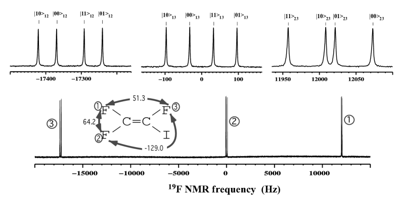
Figure 3: ¹⁹F NMR spectrum of the Iodotrifluoroethylene, measured in a field of 11.7 T. The chemical shifts are 12020 Hz, 0 Hz and -17330Hz. The inset shows the structure of the molecule and the relevant coupling constants.

The experiments were performed on a Bruker Avance II 500 MHz (11.7 Tesla) spectrometer equipped with a QXI probe with a pulsed field gradient. The resonance frequency for the ¹⁹F spins is $\approx$ 470.69 MHz.

V.2 Initialization

In the NMR experiments, the system was first prepared in a pseudopure state (PPS) Gershenfeld and Chuang (1997); Cory et al. (1997) $\rho_{000}=\frac{1-\epsilon}{8}\mathbf{1}+\epsilon|000\rangle\langle 000|$ with $\mathbf{1}$ representing the unity operator and $\epsilon\approx 10^{-5}$ the polarization, instead of the pure state $|000\rangle$. Starting from thermal equilibrium, we used spatial averaging Cory et al. (1998) to prepare the PPS; the pulse sequence Peng et al. (2002) is shown in the first part of Fig. 4.

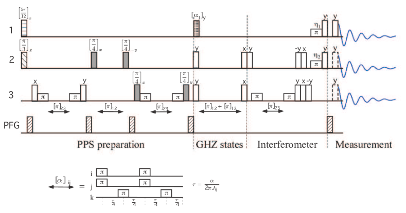
Figure 4: (Color online) Sequence of radio-frequency and field gradient pulses (PFG) used to prepare the pseudopure initial state $|000\rangle$ (first part), transform it into a GHZ-class state (second part), implement the interferometer (third part), and measure the resulting interference patterns (fourth part). The phases of the $\pi$ pulses in the interferometer, applied to qubits 1 and 2, are $\eta_{i}=\frac{\pi-\varphi_{i}}{2}$. $\left[\alpha\right]_{ij}$ denotes a pure bilinear evolution of qubits $i$ and $j$ for a duration $\frac{\alpha}{2\pi J_{ij}}$, which is realized by the refocusing scheme shown at the bottom.

In the whole experiment, we used robust strongly modulating pulses Fortunato et al. (2002); Pravia et al. (2003); Mahesh and Suter (2006) to implement all local gates (e.g., $\left[\frac{\pi}{2}\right]_{-x}^{3}$, and $\left[\pi\right]_{x}^{1,2}$ etc.). In order to confirm the state preparation, we performed a complete state tomography Chuang et al. (1998) to reconstruct the experimentally normalized relevant pure part $\rho_{exp}$ of the density matrix $\rho$: $\rho_{exp}\equiv\rho-\frac{1-\epsilon}{8}\mathbf{1}$, which is shown in Fig. 5. The experimentally determined state fidelity Uhlmann (2000) was

$$F(\rho_{th},\rho_{exp})=Tr(\sqrt{\sqrt{\rho_{th}}\rho_{exp}\sqrt{\rho_{th}}})\approx 0.99.$$

With respect to scale-indenpent NMR observations and unitary evolution, a pseudo-pure state is equivalent to the corresponding pure state Vandersypen et al. (2000); Das et al. (2003); Laflamme et al. (2002a); Ramanathan et al. (2004); Negrevergne et al. (2004); Laflamme et al. (2002b); Laflamme et al. (1998); Knill et al. (1997); Jones (2000). Therefore, we focus on the relevant pure part $\rho_{exp}$ of the pseudo-pure state in the remaining sections.

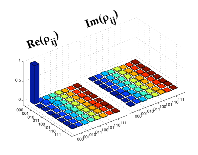
Figure 5: (Color online) Experimentally measured relevant pure part $\rho_{exp}$ of the prepared pseudo-pure state $\rho_{000}$ reconstructed by tomography. The rows and columns are numbered with the computational basis states.

V.3 Preparation of the 3-qubit source

The 3-qubit states $|\xi\rangle=\sum_{i,j,k}a_{ijk}|ijk\rangle$ of Eq. (5) were prepared from $|000\rangle$ using the quantum circuit of Fig. 6. The resulting coefficients are

$$a_{ijk}=\cos(\frac{\alpha_{1}}{2}-\frac{\pi}{2}i)\cos(\frac{\alpha^{(i)}_{2}}{2}-\frac{\pi}{2}j)\cos(\frac{\alpha^{(ij)}_{3}}{2}-\frac{\pi}{2}k).$$

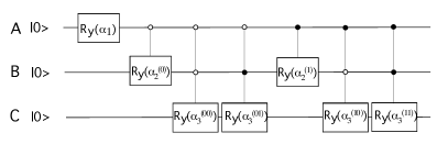
Figure 6: Quantum circuit to prepare a pure 3-particle source state $|\xi\rangle_{ABC}$. Horizontal lines represent qubits; time runs from left to right. Conditionality on the other qubits being in the $|1\rangle$ and $|0\rangle$ state are represented by filled and empty circles, respectively.

If we choose $\alpha^{(0)}_{2}=\alpha^{(00)}_{3}=\alpha^{(01)}_{3}=\alpha^{(10)}_{3}=0$ and $\alpha^{(1)}_{2}=\alpha^{(11)}_{3}=\pi$, we obtain a GHZ-class state

$$|\xi\rangle_{GHZ}=\cos\frac{\alpha_{1}}{2}|000\rangle+\sin\frac{\alpha_{1}}{2}|111\rangle.$$ (17)

The corresponding pulse sequence is represented in the second part of Fig. 4. This type of states contains only tripartite entanglement, no bipartite entanglement.

With $\alpha^{(1)}_{2}=\alpha^{(01)}_{3}=\alpha^{(10)}_{3}=\alpha^{(11)}_{3}=0$ and $\alpha^{(00)}_{3}=\pi$, we obtain a W-class state

$$|\xi\rangle_{W} = \cos\frac{\alpha_{1}}{2}\cos\frac{\alpha^{(0)}_{2}}{2}|001\rangle+$$ (18)

$$\cos\frac{\alpha_{1}}{2}\sin\frac{\alpha^{(0)}_{2}}{2}|010\rangle+\sin\frac{\alpha_{1}}{2}|100\rangle.$$

These states contain only bipartite entanglement, but no tripartite entanglement.

For $\alpha^{(1)}_{2}=\alpha^{(01)}_{3}=\alpha^{(10)}_{3}=\alpha^{(11)}_{3}=0$, we obtain the state

$$|\xi\rangle_{int} = \cos\frac{\alpha_{1}}{2}\cos\frac{\alpha^{(0)}_{2}}{2}\cos\frac{\alpha^{(00)}_{3}}{2}|000\rangle$$ (19)

$$+\cos\frac{\alpha_{1}}{2}\cos\frac{\alpha^{(0)}_{2}}{2}\sin\frac{\alpha^{(00)}_{3}}{2}|001\rangle$$

$$+\cos\frac{\alpha_{1}}{2}\sin\frac{\alpha^{(0)}_{2}}{2}|010\rangle+\sin\frac{\alpha_{1}}{2}|100\rangle.$$

It has tripartite as well as bipartite entanglement. These states are intermediate between the GHZ-class and the W-class states. We call them the intermediate-class states.

V.4 Implementation of the Interferometer

To implement the interferometer shown in Fig. 1, we first need to determine the relevant eigenbasis $\{|\Phi_{0}\rangle,|\Phi_{1}\rangle\}_{BC}$ of the reduced density operator $\rho_{BC}$ of the $BC$ subsystem. Table 1 lists the eigenbases for the three initial states that we consider in this context.

Table 1: The preferred basis $\{|\Phi_{0}\rangle,|\Phi_{1}\rangle\}_{BC}$ in the interferometer (see Fig. 1) for three different classes of input states. For the intermediate-class states, the coefficients are $a_{1}=\cos\frac{\theta_{1}}{2},a_{2}=\sin\frac{\theta_{1}}{2}\sin\frac{\theta_{3}}{2},a_{3}=\sin\frac{\theta_{1}}{2}\cos\frac{\theta_{3}}{2}$ for $|\Phi_{0}\rangle$ and $a^{\prime}_{1}=-\sin\frac{\theta_{1}}{2},a^{\prime}_{2}=\cos\frac{\theta_{1}}{2}\sin\frac{\theta_{3}}{2},a^{\prime}_{3}=\cos\frac{\theta_{1}}{2}\cos\frac{\theta_{3}}{2}$ for $|\Phi_{1}\rangle$.

State class	$|\Phi_{0}\rangle$	$|\Phi_{1}\rangle$
GHZ	$|00\rangle$	$|11\rangle$
W	$|00\rangle$	$\cos\frac{\alpha^{(0)}_{2}}{2}|01\rangle+\sin\frac{\alpha^{(0)}_{2}}{2}|10\rangle$
Intermediate	$a_{1}|00\rangle+a_{2}|01\rangle+a_{3}|10\rangle$	$a^{\prime}_{1}|00\rangle+a^{\prime}_{2}|01\rangle+a^{\prime}_{3}|10\rangle$

To apply the transducer in this basis, we have to find the basis transformation between this eigenbasis and the computational basis. Writing $|\Phi_{0}\rangle$ as a general two-qubit state,

$$|\Phi_{0}\rangle = \cos\frac{\theta_{1}}{2}\cos\frac{\theta_{2}}{2}|00\rangle+\sin\frac{\theta_{1}}{2}\sin\frac{\theta_{3}}{2}|01\rangle$$ (20)

$$+\sin\frac{\theta_{1}}{2}\cos\frac{\theta_{3}}{2}|10\rangle+\cos\frac{\theta_{1}}{2}\sin\frac{\theta_{2}}{2}|11\rangle,$$

we can transform it into the computational basis state $|00\rangle$ by the transformation

$$\mathcal{R} = \left(\begin{array}[]{cccc}\cos\frac{\theta_{1}}{2}\cos\frac{\theta_{2}}{2}&\sin\frac{\theta_{1}}{2}\sin\frac{\theta_{3}}{2}&\sin\frac{\theta_{1}}{2}\cos\frac{\theta_{3}}{2}&\cos\frac{\theta_{1}}{2}\sin\frac{\theta_{2}}{2}\\ -\cos\frac{\theta_{1}}{2}\sin\frac{\theta_{2}}{2}&\sin\frac{\theta_{1}}{2}\cos\frac{\theta_{3}}{2}&-\sin\frac{\theta_{1}}{2}\sin\frac{\theta_{3}}{2}&\cos\frac{\theta_{1}}{2}\cos\frac{\theta_{2}}{2}\\ -\sin\frac{\theta_{1}}{2}\cos\frac{\theta_{2}}{2}&\cos\frac{\theta_{1}}{2}\sin\frac{\theta_{3}}{2}&\cos\frac{\theta_{1}}{2}\cos\frac{\theta_{3}}{2}&-\sin\frac{\theta_{1}}{2}\sin\frac{\theta_{2}}{2}\\ -\sin\frac{\theta_{1}}{2}\sin\frac{\theta_{2}}{2}&\cos\frac{\theta_{1}}{2}\cos\frac{\theta_{3}}{2}&-\cos\frac{\theta_{1}}{2}\sin\frac{\theta_{3}}{2}&\sin\frac{\theta_{1}}{2}\cos\frac{\theta_{2}}{2}\end{array}\right).$$ (25)

The same operator also maps the other basis states $|\Phi_{i}\rangle,i=1,2,3$ into basis states of the computational basis. For the GHZ states, the pulse sequence for the implementation of this transformation is shown in the third part of Fig. 4. Depending on the basis states $\{|\Phi_{i}\rangle\}$, a permutation of the computational basis states is required.

The preferred bases for the different states are shown in Table 1. For the GHZ-class states, the parameters are $\theta_{i}=0,(i=1,2,3)$ and the transformation operator $\mathcal{R}$ simplifies to CNOT₃₂. For the W-class states, the parameters are $\theta_{1}=\theta_{2}=0,\theta_{3}=-\alpha^{(0)}_{2}$. For the intermediate-class states, the parameters $\theta_{i}$ are determined by the the two non-zero eigenvalues of the reduced density matrix $\rho_{BC}$,

$$\lambda_{\pm}=\frac{1}{2}(1\pm\sqrt{1-4A\sin^{2}\frac{\alpha_{1}}{2}},$$

where

$$A=\cos^{2}\frac{\alpha_{1}}{2}(\cos^{2}\frac{\alpha_{2}^{(0)}}{2}\sin^{2}\frac{\alpha_{3}^{(00)}}{2}+\sin^{2}\frac{\alpha_{2}^{(0)}}{2}).$$

In terms of these parameters, we find for the parameters $\theta_{i}$ in the basis transformation $\mathcal{R}$

$$\tan^{2}\frac{\theta_{1}}{2}=-\frac{\lambda_{-}-A}{\lambda_{+}-A},\;\;\;\theta_{2}=0$$

and

$$\tan\frac{\theta_{3}}{2}=\cot\frac{\alpha_{2}^{(0)}}{2}\sin\frac{\alpha_{3}^{(00)}}{2}.$$

V.5 Measurement

After the interferometer, the output state of the complete 3-qubit system is

$$|\psi_{out}\rangle=U_{A}(\varphi_{1})\otimes\mathcal{R}^{-1}P^{\dagger}U_{BC}(\varphi_{2})P\mathcal{R}|\xi\rangle,$$ (26)

where $P$ is the relevant permutation matrix. For these states, we measure the joint probabilities $p(|i\rangle_{A}|\Phi_{j}\rangle_{BC})$ for detecting particle $A$ on port $|i\rangle$ and particles $B$ and $C$ on port $|\Phi_{j}\rangle$ of the interferometer. This probability can be written as the projection of the output states onto the measurement basis

$$p(|i\rangle_{A}|\Phi_{j}\rangle_{BC})=|_{BC}\langle\Phi_{j}|_{A}\langle i|\psi_{out}\rangle|^{2}.$$ (27)

This expression can be evaluated in the computational basis $|ijk\rangle$ by using the transformation operator $\mathcal{R}$:

$$p(|i\rangle_{A}|\Phi_{j}\rangle_{BC})=|_{BC}\langle jk|_{A}\langle i|\mathcal{R}|\psi_{out}\rangle|^{2}.$$ (28)

The single-particle probabilities of particle $A$ are

$$p(|i\rangle_{A})=_{A}\langle i|Tr_{BC}(|\psi_{out}\rangle\langle\psi_{out}|)|i\rangle_{A}.$$ (29)

Figure 7: Experimental spectra of the three ¹⁹F spins (corresponding to qubits 1, 2 and 3 from right to left) for the GHZ state when $\varphi=\varphi_{1}=\varphi_{2}=-\pi/2$.

To determine the probabilities, we measured the populations of all eight computational basis states by first deleting coherences with a field gradient pulse and then applying selective readout pulses to the individual qubits. This procedure is denoted by the last part of Fig. 4. The dashed read-out pulses indicate that the three pulses were applied in three separate experiments. From each of the three FIDs, we obtain a spectrum of the corresponding spin with four resonance lines after Fourier transformation. Fig. 7 show representative spectra for the case of the GHZ state and a phase shift of $\varphi=\varphi_{1}=\varphi_{2}=-\pi/2$ in the interferometer.

As the path length of the interferometer arms is changed, interference between the two paths changes the populations of the different states. This oscillation can be observed directly in the NMR spectra, as shown in Fig. 8, where we have plotted the variation of the subspectrum of qubit 1 as a function of the phase $\varphi$ for the GHZ state.

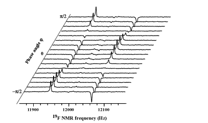
Figure 8: Variation of the spectrum of qubit 1 with the interferometer phase $\varphi$ for the GHZ state.

The relevant populations were obtained from the spectra by integrating over the resonance lines. Fig. 9 shows interferograms for some of the populations (equal to the probabilities $p(|i\rangle_{A}|\Phi_{j}\rangle_{BC}$) for the GHZ-state (left hand side) and a product state (right hand side). Clearly, the maximally entangled state shows high visibility fringes, while the variation of the populations essentially vanishes for the product state.

We extracted the visibility $V_{A(BC)}$ from the interferograms of the populations $p(|i\rangle_{A}|\Phi_{j}\rangle_{BC})$ by Eq. (9). The single-particle probabilities $p(|i\rangle_{A})$ were obtained by summing the the populations related to the state $|i\rangle_{A}$, from which we obtained the singe-particle visibility $V_{A}$. The results is summarized in the next subsection.

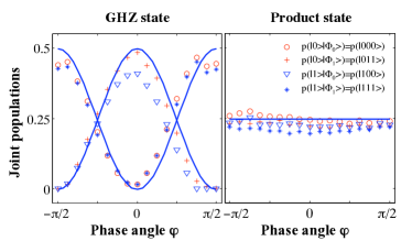
Figure 9: (Color online) Relevant joint populations reconstructed from the experimental data for (a) the GHZ state and (b) the product state.

In addition to the visibility, we measured the predictability $\mathcal{P}_{A}$. According to Eq. (8), it is given as the expectation value of the observable $\sigma_{z}^{(A)}$, i.e. the population difference of particle $A$. We measured it by applying a field gradient pulse that destroyed the coherences and a subsequent readout pulse $\left[\frac{\pi}{2}\right]_{y}^{A}$ that converted $\sigma_{z}^{(A)}$ into $\sigma_{x}^{(A)}$, which was then recorded as the FID. After Fourier transformation, we integrated over the relevant resonance lines in the spectrum. The absolute value of this integral corresponds to the predictability $\mathcal{P}_{A}$.

V.6 Experimental results

Fig. 10 summarizes the experimental results for three different classes of states by plotting the degree of local vs. nonlocal character for each case. According to section II, they should be related by the complementarity relation $V_{A(BC)}^{2}+S_{A}^{2}=1$ for the pure three-qubit states, where $S_{A}=\sqrt{V_{A}^{2}+P_{A}^{2}}$ quantifies the local character and $V_{A(BC)}$ the nonlocal character. Clearly, the experimental data points (circles) agree well with the theoretical prediction (solid curves). In the first system (GHZ), the non-local character is due exclusively to tripartite entanglement; in the second system (W), it arises from bipartite entanglement, and in the third case, we have a combination of both types of entanglement.

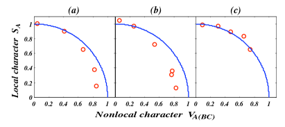
Figure 10: (Color online) Experimental verification of the complementarity relation of $V_{A(BC)}^{2}+S_{A}^{2}=1$ in a pure three-qubit system: (a) for GHZ-class states of Eq. (17), (b) for W-class states of Eq. (18) and (c) for intermediate-class states of Eq. (19). Solid curves represent the theoretical complementarity relation of local character $S_{A}$ versus nonlocal property $V_{A(BC)}$. Experimental results are indicated by circles.

The deviation between the experimental and theoretical values is primarily due to the inhomogeneity of the radio frequency field and the static magnetic field, imperfect calibration of radio frequency pulses, and signal decay during the experiments. The experimental errors are bigger for states with predominantly ”non-local” character. This is well compatible with the general expectation that nonlocal states are less robust and is observed even for the initial state preparation, where the measured fidelity is lower for the nonlocal states. For example, the experimental fidelity of the GHZ state $\frac{1}{\sqrt{2}}(|000\rangle+|111\rangle)$ with $\alpha_{1}=\pi/2$ in Eq. (17) is about 0.97, compared to the 0.99 fidelity of the product state $|000\rangle$ with $\alpha_{1}=0$ in Eq. (17).

VI Conclusion

While complementarity was first introduced as a qualitative concept, it was recently found that in many situations, quantitative complementarity relations can be formulated. Here, we have quantitatively compared the local versus nonlocal character of the quantum states of three coupled qubits (spins 1/2).

For the experimental measurements, we used a system of three coupled nuclear spins in a liquid-state NMR spectrometer. The degree of local vs. nonlocal character was measured by constructing a suitable four-way interferometer and utilizing a specific property of pure three-qubit states: In any two-qubit subsystem $\rho_{BC}$, at most two eigenvectors of the density matrix have non-zero eigenvalues. This allowed us to quantify the local character of the system by measuring the polarization of the (arbitrary) particle $A$ and the nonlocal character via a measurement of the entanglement between the single qubit $A$ and the subsystem $BC$. While the interferometer only uses four channels, they were chosen in such a way that the measurement results quantify the complete entanglement of the three-qubit system, including bipartite as well as tripartite contributions.

Here we have restricted our theoretical treatment to cases where the three-qubit system is described in a pure quantum state. In an experiment, the prepared states inevitably involve some mixture less or more. Naturally, the question arises as to what happens when the system is initially a mixed state. As discussed in Ref. Jakob and Bergou (2003) and Peng et al. (2005) for a bipartite system, a weaker statement for the complementarity of Eq. (4) is believed in the form of an inequality $C_{A(BC)}^{2}(\rho)+S_{A}^{2}(\rho)\leq 1$ for the most general case of a mixed three-qubit system. However, similar to the case of a bipartite system Jakob and Bergou (2003); Peng et al. (2005), there is no corresponding inequality for the visibility $V_{A(BC)}$ in the mixed three-qubit states because the definition of $V_{A(BC)}$ by Jeager et al. Jaeger et al. (1993, 1995) is unfeasible and the direct relation between the concurrence $C_{A(BC)}$ and the visibility $V_{A(BC)}$ ceases to exist for mixed states.

The complementarity relation that we have verified here, can be used to measure the degree of entanglement by measuring only the single-particle character of a given state. Our measurements extend earlier tests of complementarity that were done in one- or two-qubit systems Taylor (1909); Mittelstaedt et al. (1987); Moellenstedt and Joensson (1959); Tonomura et al. (1989); Zeilinger et al. (1988); Eichmann et al. (1993); Carnal and Mlynek (1991); Kim et al. (2000); Scully et al. (1991); Abouraddy et al. (2001); Dürr et al. (1998a, b); Peng et al. (2003, 2005); Zhu et al. (2001). This experiment may thus be considered as a first step towards establishing and testing quantitative complementarity relations in multi-qubit systems.

ACKNOWLEDGMENTS

This work is supported by the DFG through Su 192/19-1, the Alexander von Humboldt Foundation and the Marie Curie program of the EU.

References

- Bohr (1928) N. Bohr, Naturwiss. 16, 245 (1928).
- Taylor (1909) G. Taylor, Proc. Camb. Phil. Soc. 15, 114 (1909).
- Dempster and Batho (1927) A. J. Dempster and H. F. Batho, Phys. Rev. 30, 644 (1927).
- Moellenstedt and Joensson (1959) G. Moellenstedt and C. Joensson, Zeitschrift fuer Physik A Hadrons and Nuclei 155, 472 (1959).
- Tonomura et al. (1989) A. Tonomura, J. Endo, T. Matsuda, T. Kawasaki, and H. Ezawa, Am. J. Phys. 57, 117 (1989).
- Zeilinger et al. (1988) A. Zeilinger, R. Gähler, C. G. Shull, W. Treimer, and W. Mampe, Rev. Mod. Phys. 60, 1067 (1988).
- Eichmann et al. (1993) U. Eichmann, J. C. Bergquist, J. J. Bollinger, J. M. Gilligan, W. M. Itano, D. J. Wineland, and M. G. Raizen, Phys. Rev. Lett. 70, 2359 (1993).
- Carnal and Mlynek (1991) O. Carnal and J. Mlynek, Phys. Rev. Lett. 66, 2689 (1991).
- Arndt et al. (1999) M. Arndt, O. Nairz, J. Voss-Andreae, C. Keller, G. V. der Zouw, and A. Zeilinger, Nature 401, 680 (1999).
- Wootters and Zurek (1979) W. K. Wootters and W. H. Zurek, Phys. Rev. D 19, 473 (1979).
- Bartell (1980) L. S. Bartell, Phys. Rev. D 21, 1698 (1980).
- Greenberger and Yasin (1988) D. M. Greenberger and A. Yasin, Phys. Lett. A 128, 391 (1988).
- Mandel (1991) L. Mandel, Opt. Lett. 16, 1882 (1991).
- Jaeger et al. (1995) G. Jaeger, A. Shimony, and L. Vaidman, Phys. Rev. A 51, 54 (1995).
- Englert (1996) B.-G. Englert, Phys. Rev. Lett. 77, 2154 (1996).
- Englert and Bergou (2000) B.-G. Englert and J. A. Bergou, Opt. Comm. 179, 337 (2000).
- Englert et al. (2007) B.-G. Englert, D. Kaszlikowski, L. C. Kwek, and W. H. Chee, arXiv:0710.0179v1 [quant-ph] (2007).
- Jaeger et al. (1993) G. Jaeger, M. A. Horne, and A. Shimony, Phys. Rev. A 48, 1023 (1993).
- Scully and Zubairy (1997) M. O. Scully and M. S. Zubairy, Quantum Optics (Cambridge University Press, Cambridge, 1997).
- Scully et al. (1991) M. O. Scully, B.-G. Englert, and H. Walther, Nature 351, 111 (1991).
- Schwindt et al. (1999) P. D. D. Schwindt, P. G. Kwiat, and B.-G. Englert, Phys. Rev. A 60, 4285 (1999).
- Kim et al. (2000) Y.-H. Kim, R. Yu, S. P. Kulik, Y. Shih, and M. O. Scully, Phys. Rev. Lett. 84, 1 (2000).
- Abouraddy et al. (2001) A. F. Abouraddy, M. B. Nasr, B. E. A. Saleh, A. V. Sergienko, and M. C. Teich, Phys. Rev. A 63, 063803 (2001).
- Pryde et al. (2004) G. J. Pryde, J. L. O’Brien, A. G. White, S. D. Bartlett, and T. C. Ralph, Phys. Rev. Lett. 92, 190402 (2004).
- Dürr et al. (1998a) S. Dürr, T. Nonn, and G. Rempe, Nature 395, 33 (1998a).
- Dürr et al. (1998b) S. Dürr, T. Nonn, and G. Rempe, Phys. Rev. Lett. 81, 5705 (1998b).
- Peng et al. (2003) X. Peng, X. Zhu, X. Fang, M. Feng1, M. Liu, and K. Gao, J. Phys. A: Math. Gen. 36, 2555 (2003).
- Peng et al. (2005) X. Peng, X. Zhu, D. Suter, J. Du, M. Liu, and K. Gao, Phys. Rev. A 72, 052109 (2005).
- Zhu et al. (2001) X. Zhu, X. Fang, X. Peng, M. Feng, K. Gao, and F. Du, J. Phys. B: At. Mol. Opt. Phys. 34, 4349 (2001).
- Oppenheim et al. (2003) J. Oppenheim, K. Horodecki, M. Horodecki, P. Horodecki, and R. Horodecki, Phys. Rev. A 68, 022307 (2003).
- Saleh et al. (2000) B. E. A. Saleh, A. F. Abouraddy, A. V. Sergienko, and M. C. Teich, Phys. Rev. A 62, 043816 (2000).
- Bose and Home (2002) S. Bose and D. Home, Phys. Rev. Lett. 88, 050401 (2002).
- Jakob and Bergou (2003) M. Jakob and J. A. Bergou, arXiv:quant-ph/0302075v1 (2003).
- Jaeger et al. (2003) G. Jaeger, A. V. Sergienko, B. E. A. Saleh, and M. C. Teich, Phys. Rev. A 68, 022318 (2003).
- Tessier (2005) T. E. Tessier, Foundations of Physics Letters 18, 107 (2005).
- Rungta et al. (2001) P. Rungta, V. Bužek, C. M. Caves, M. Hillery, and G. J. Milburn, Phys. Rev. A 64, 042315 (2001).
- Rungta and Caves (2003) P. Rungta and C. M. Caves, Phys. Rev. A 67, 012307 (2003).
- Wootters (1998) W. K. Wootters, Phys. Rev. Lett. 80, 2245 (1998).
- Coffman et al. (2000) V. Coffman, J. Kundu, and W. K. Wootters, Phys. Rev. A 61, 052306 (2000).
- Gershenfeld and Chuang (1997) N. Gershenfeld and I. Chuang, Science 275, 350 (1997).
- Cory et al. (1997) D. Cory, A. Fahmy, and T. Havel, Proc. Natl. Acad. Sci. 94, 1634 (1997).
- Cory et al. (1998) D. G. Cory, M. D. Price, and T. F. Havel, Physica D: Nonlinear Phenomena 120, 82 (1998).
- Peng et al. (2002) X. Peng, X. Zhu, X. Fang, M. Feng, X. Yang, M. Liu, and K. Gao, arXiv.org:quant-ph/0202010 (2002).
- Fortunato et al. (2002) E. M. Fortunato, M. A. Pravia, N. Boulant, G. Teklemariam, T. F. Havel, and D. G. Cory, J. Chem. Phys. 116, 7599 (2002).
- Pravia et al. (2003) M. A. Pravia, N. Boulant, J. Emerson, E. M. F. andTimothy F. Havel, R. Martinez, and D. G. Cory, J. Chem. Phys. 119, 9993 (2003).
- Mahesh and Suter (2006) T. S. Mahesh and D. Suter, Phys. Rev. A 74, 062312 (2006).
- Chuang et al. (1998) I. L. Chuang, N. Gershenfeld., M. G. Kubinec, and D. W. Leung, Proceedings of the Royal Society A: Mathematical, Physical and Engineering Sciences 454, 447 (1998).
- Uhlmann (2000) A. Uhlmann, Rep. Math. Phys. 45, 407 (2000).
- Vandersypen et al. (2000) L. M. Vandersypen, C. S. Yannoni, and I. L. Chuang, arXiv:quant-ph/0012108 (2000).
- Das et al. (2003) R. Das, A. Mitra, S. V. Kumar, and A. Kumar, arXiv:quant-ph/0307240v1 (2003).
- Laflamme et al. (2002a) R. Laflamme, E. Knill, D. Cory, E. Fortunato, T. Havel, C. Miquel, R. Martinez, C. Negrevergne, G. Ortiz, M. Pravia, et al., arXiv:quant-ph/0207172v1 (2002a).
- Ramanathan et al. (2004) C. Ramanathan, N. Boulant, Z. Chen, D. G. Cory, I. Chuang, and M. Steffen, Quantum Information Processing 3, 15 (2004).
- Negrevergne et al. (2004) C. Negrevergne, R. Somma, G. Ortiz, E. Knill, and R. Laflamme, arXiv:quant-ph/0410106 (2004).
- Laflamme et al. (2002b) R. Laflamme, D. G. Cory, C. Negrevergne, and L. Viola, Quantum Information and Computation 2, 166 (2002b).
- Laflamme et al. (1998) R. Laflamme, E. Knill, W. Zurek, P. Catasti, and S. Mariappan, Phil.Trans.Roy.Soc.Lond. A 356, 1941 (1998).
- Knill et al. (1997) E. Knill, I. Chuang, and R. Laflamme, arXiv:quant-ph/9706053 (1997).
- Jones (2000) J. A. Jones, arXiv:quant-ph/0009002 (2000).
- Mittelstaedt et al. (1987) P. Mittelstaedt, A. Prieur, and R. Schieder, Foundations of Physics 17, 891 (1987).