Approximate Sparse Decomposition Based on Smoothed $\ell^{0}$-Norm

Abstract

In this paper, we propose a method to address the problem of source estimation for Sparse Component Analysis (SCA) in the presence of additive noise. Our method is a generalization of a recently proposed method (SL0), which has the advantage of directly minimizing the $\ell^{0}$-norm  instead of $\ell^{1}$-norm, while being very fast. SL0 is based on minimization of the smoothed $\ell^{0}$-norm  subject to ${\bf A}{\bf s}={\bf x}$. In order to better estimate the source vector for noisy mixtures, we suggest then to remove the constraint ${\bf A}{\bf s}={\bf x}$, by relaxing exact equality to an approximation (we call our method Smoothed $\ell^{0}$-norm  Denoising or SL0DN). The final result can then be obtained by minimization of a proper linear combination of the smoothed $\ell^{0}$-norm and a cost function for the approximation. Experimental results emphasize on the significant enhancement of the modified method in noisy cases.

Index Terms—  atomic decomposition, sparse decomposition, sparse representation, over-complete signal representation, sparse source separation

1 Introduction

Blind source separation (BSS) consists of detecting the underlying source signals within some observed mixtures of them without any prior information about the sources or the mixing system. Let ${\bf x}\in\mathbb{R}^{n}$ be the vector of observed mixtures and ${\bf s}\in\mathbb{R}^{m}$ denote the vector of unknown source signals. The mixing equation for the linear instantaneous noisy model will be:

$${\bf x}={\bf A}{\bf s}+{\bf n}$$ (1)

where A is the $n\times m$ unknown mixing matrix and n denotes the additive noise vector. The aim of BSS is then to estimate ${\bf s}$ from observed data x without any knowledge of the mixing matrix, A, or the source signals.

In the determined case, when $n$ $\geq$ $m$, the problem can be successfully solved using Independent Component Analysis (ICA) [1]. However, in the underdetermined (or over-complete) cases where fewer observations than sources are provided, even if $\bf A$ is known, there are infinitely many solutions to the problem since the number of unknowns exceeds the number of equations. This ill-posedness could be resolved by the assumption of ‘Sparsity’, i.e. resulting in non totally blind source separation problem. A signal is considered to be sparse when only a few of its samples take significant values. Thus, among all possible solutions of (1) we seek the sparsest one, which has then minimum number of nonzero components, i.e. minimum $\ell^{0}$-norm.

SCA can also be viewed as the problem of representing a signal ${\bf x}\in\mathbb{R}^{n}$ as a linear combination of $m$ vectors, called atoms [2]. The atoms $\{{\mbox{\boldmath$\varphi$}}_{i}\}_{i=1}^{m}$ collectively form a dictionary, $n\times m$ matrix, over which the signal is to be decomposed.There are special interests in the cases where $m>n$ (refer for example to [3] and the references in it). Again we have the problem of finding the sparsest solution of the set of underdetermined linear equations ${\bf x}=\sum_{i=1}^{m}s_{i}{\mbox{\boldmath$\varphi$}}_{i}$ where ${\mbox{\boldmath$\Phi$}}\triangleq[{\mbox{\boldmath$\varphi$}}_{1},\dots,{\mbox{\boldmath$\varphi$}}_{m}]$ is the dictionary of $m$ atoms. This problem is also called ‘atomic decomposition’ and has many potential applications in diverse fields of science [3].

The general Sparse Component Analysis (SCA) problem consists of two steps: first estimating the mixing matrix, and then finding the sparsest source vector, assuming the mixing matrix to be known. The first step can be accomplished by means of clustering methods [4]. In this paper, we focus our attention on the second step; that is for a given mixing matrix, we wish to find the solution to the following minimization problem:

$$\hat{{\bf s}}=\mathrm{argmin}\|{\bf s}\|_{0}\qquad\textrm{subject to }~{}{\bf x}={\bf A}{\bf s}$$ (2)

where $\|{\bf s}\|_{0}$ denotes the number of non-zero elements of ${\bf s}$ (and is usually called the $\ell^{0}$-norm of ${\bf s}$).

So far, several algorithms such as Basis Pursuit (BP)  [5, 6] and Matching Pursuit (MP)  [2, 4] have been proposed to approximate the solution of (2). The former is based on the observation that for most large underdetermined systems of linear equations the minimal $\ell^{1}$-norm ($\sum_{i}|s_{i}|$ ) solution is also the sparsest solution [6]. The minimization of $\ell^{1}$-norm can be efficiently solved using Linear Programming (LP) techniques [7]. Despite all recent developments, computational efficiency has still remained as a main concern.

Recently in  [8], the idea of using smoothed $\ell^{0}$-norm  (SL0) was introduced. More precisely this algorithm minimizes a smooth approximation of the $\ell^{0}$-norm denoted by $m-F_{\sigma}({\bf s})$, and the approximation tends to equality when $\sigma\rightarrow 0$. The algorithm then sequentially solves the problem:

$$\mathrm{maximize}~{}F_{\sigma}({\bf s})\quad\mathrm{s.t.}\quad{\bf A}{\bf s}={\bf x}$$ (3)

for a decreasing sequence of $\sigma$.

This approximation accommodates for both continuous optimization techniques to estimate the sparsest solution of (2) and a noise-tolerant algorithm. The idea turned out to be both efficient and accurate, i.e. providing a better accuracy than $\ell^{1}$-norm  minimization algorithms while being about two orders of magnitude faster [8] than LP.

However, the proposed algorithm has not been designed for the noisy case (1), where a noise vector, n, has been added to the observed mixture x. In this paper, we will try to generalize the proposed method to this noisy case by removing the ${\bf A}{\bf s}={\bf x}$ constraint and relaxing the exact equality to an approximation. In sparse decomposition viewpoint, this means an approximate sparse decomposition of a signal on an over-complete dictionary. The final algorithm will then be an iterative minimization of a proper linear combination of smoothed $\ell^{0}$-norm and $\|{\bf A}{\bf s}-{\bf x}\|_{2}^{2}$.

This paper is organized as follows. Section 2 discusses the main idea of the proposed method. Section 3 gives a formal statement of the final algorithm. Finally, experimental results are presented in Section 4.

2 Main Idea

As stated in the previous section, when the dimensions increase, finding the minimum $\ell^{0}$-norm solution of (2) is impractical for two reasons. Firstly because $\ell^{0}$-norm of a vector is a discontinuous function of its elements and leads to an intractable combinatorial optimization, and secondly because of the solution being highly sensitive to noise. The idea of [8] is then to replace the $\ell^{0}$-norm by continuous function, which approximates Kronecker delta function, and use optimization techniques to minimize it subject to ${\bf A}{\bf s}={\bf x}$, as a constraint. For example, consider the Gaussian like function:

$$F_{\sigma}({\bf s})=\sum_{i=1}^{m}\exp{(-s_{i}^{2}/2\sigma^{2})}$$ (4)

where $s_{i}$ denotes the $i$-th element of vector ${\bf s}$. For sufficiently small values of $\sigma$, $F_{\sigma}(s)$ tends to count the number of zero elements of the vector s. Thus we have:

$$\|{\bf s}\|_{0}=m-\lim_{\sigma\to 0}F_{\sigma}({\bf s})$$ (5)

where $m$ is the dimension of the vector ${\bf s}$. The sparsest solution of (2) can then be approximated by the solution of the following minimization problem:

$$\hat{{\bf s}}=\mathrm{argmin}~{}(m-F_{\sigma}({\bf s}))\qquad\textrm{subject to }~{}{\bf x}={\bf A}{\bf s}$$ (6)

The above minimization task can be accomplished using common gradient type (e.g. steepest descent) algorithms. Note that the value of $\sigma$ determines how smooth the function $F_{\sigma}$ is; the smaller the value of $\sigma$, the better the estimation of $\|{\bf s}\|_{0}$ but the larger the probability of being trapped in local minima of the cost function. The idea of [8] for escaping from local minima is then to use a decreasing set of values for $\sigma$ in each iteration. More precisely for each value of $\sigma$ the minimization algorithm is initiated with the minimizer of the $F_{\sigma}({\bf s})$ for the previous (larger) value of $\sigma$.

Now consider a more realistic case where a noise vector, n, has been added to the observed mixture, as in (1). Here we notice that we have an uncertainty on exact value of the observed vector and it seems reasonable to remove the ${\bf x}={\bf A}{\bf s}$ constraint and reduce it to ${\bf x}\approx{\bf A}{\bf s}$. This idea is based on the observation that in presence of considerable noise, this constraint may lead to a totally different sparse decomposition. Thus we wish to minimize two terms; $\|{\bf A}{\bf s}-{\bf x}\|_{2}$ as cost of approximation, and the smoothed $\ell^{0}$-norm ($m-F_{\sigma}({\bf s})$), as the measure of sparsity.

For the sake of simplicity, we choose $\|{\bf A}{\bf s}-{\bf x}\|_{2}^{2}$ as the cost of approximation. Therefore, the idea will naturally leads us to the following minimization problem:

$$\hat{{\bf s}}=\mathrm{argmin}~{}J_{\sigma}({\bf s})=(m-F_{\sigma}({\bf s}))+\lambda~{}\|{\bf A}{\bf s}-{\bf x}\|_{2}^{2}$$ (7)

where $\lambda>0$, represents a compromise between the two terms of our cost function; sparsity and equality condition. Intuitively, we may expect that for less noisy mixtures, the value of $\lambda$ should be greater than that of observations with high noise quantity. Further discussion on the choice of $\lambda$ is left to Section 4.

Another advantage of removing ${\bf x}={\bf A}{\bf s}$ constraint appears when the dictionary matrix, ${\bf A}$, is not full rank. In this case satisfying the exact equality constraint for observed vectors, which are not in column space of $\bf A$ is impossible and as a result the previous algorithm fails to find any answer.

3 Final Algorithm

The final algorithm is shown in Fig 1. We call our algorithm SL0 DeNoising (SL0DN). As seen in the algorithm, the final values of the previous estimation are used for the initialization of the next steepest descent step. The decreasing sequence of $\sigma$ is used to escape from getting trapped into local minima.

Direct calculations show that:

$$\Delta{\bf s}=\frac{\partial J_{\sigma}({\bf s})}{\partial{\bf s}}=\lambda(2{\bf A}^{T}({\bf A}{\bf s}-{\bf x}))$$

$$+\frac{1}{\sigma^{2}}[s_{1}e^{(-s_{1}^{2}/2\sigma^{2})},\dots,s_{m}e^{(-s_{m}^{2}/2\sigma^{2})}]^{T}$$ (8)

In the minimization part, the steepest descent with variable step-size ($\mu$) has been applied: If $\mu$ is such that $J_{\sigma}({\bf s}-\mu\Delta{{\bf s}})<J_{\sigma}({\bf s})$ we multiply it by 1.2 for the next iteration, otherwise it is multiplied by 0.5.

    • Initialization: 1. Let ${\bf\hat{s}}_{0}={\bf A}^{T}({\bf A}{\bf A}^{T})^{-1}{\bf x}$. 2. Choose a suitable value for $\lambda$ as a function of $\sigma_{\mathrm{n}}$. The value of $\sigma_{\mathrm{n}}$ for a set of observed mixtures may be estimated either directly from the observed mixtures (see for example [9] and references therein) or using a bootstrap method (discussed in experiment 1 of Section 4). 3. Choose a suitable decreasing sequence for $\sigma$,
$[\sigma_{1}\ldots\sigma_{K}]$. and a sufficiently small value for the step-size parameter, $\mu$. • For $k=1,\dots,K$: 1. Let $\sigma=\sigma_{k}$. 2. Minimize (approximately) the function $J_{\sigma}({\bf s})$ using $L$ iterations of the steepest descent algorithm: – Initialization: ${\bf s}\leftarrow{\bf\hat{s}}_{k-1}$. – for $j=1\dots L$ (loop $L$ times): (a) Let: $\Delta{\bf s}=\lambda(2{\bf A}^{T}({\bf A}{\bf s}-{\bf x}))+\frac{1}{\sigma^{2}}[s_{1}e^{(-s_{1}^{2}/2\sigma^{2})},\dots,s_{m}e^{(-s_{m}^{2}/2\sigma^{2})}]^{T}$ (b) If $J_{\sigma}({\bf s}-\mu\Delta{{\bf s}})<J_{\sigma}({\bf s})$ let $\rho=1.2$ else $\rho=0.5$. (c) Let ${\bf s}\leftarrow{\bf s}-\mu\Delta{\bf s}$ (d) Let $\mu\leftarrow\mu\times\rho$. (variable step-size) (e) Set ${\bf\hat{s}}_{k}\leftarrow{\bf s}$. • Final answer is ${\bf\hat{s}}={\bf\hat{s}}_{K}$.    

Fig. 1: The final algorithm of SL0DN.

4 Experimental Results

In this section we investigate the performance of the proposed method and present our simulation results. Since our framework is a generalization of the idea presented in [8], the practical considerations in that paper can be directly imported into our framework.

In [8], it has been experimentally shown that SL0 is about two orders of magnitude faster than the state-of-the-art interior-point LP solvers [7], while being more accurate. We provide the comparison results of our method with the SL0 method. Moreover a comparison with Basis Pursuit Denoising will be presented.

In all experiments, sparse sources have been artificially generated using a Bernoulli-Gaussian model: each source is ‘active’ with probability $p$, and is ‘inactive’ with probability $1-p$. If it is active, its value is modeled by a zero-mean Gaussian random variable with variance $\sigma^{2}_{\mathrm{on}}$; if it is not active, its value is modeled by a zero-mean Gaussian random variable with variance $\sigma^{2}_{\mathrm{off}}$, where $\sigma^{2}_{\mathrm{off}}\ll\sigma^{2}_{\mathrm{on}}$. Consequently, each $s_{i}$ is distributed as:

$$s_{i}\sim p\cdot\mathcal{N}(0,\sigma_{\mathrm{on}})+(1-p)\cdot\mathcal{N}(0,\sigma_{\mathrm{off}}),$$ (9)

Sparsity implies that $p\ll 1$. We considered $p=0.1$, $\sigma_{\mathrm{off}}=0.01$ and $\sigma_{\mathrm{on}}=1$. Elements of the mixing matrix, A, and noise vector, n, were also considered to have normal distributions with standard deviation of 1 and $\sigma_{\mathrm{n}}$, respectively. As in [8], the set of decreasing values for $\sigma$ was fixed to $[1,0.5,0.2,0.1,0.05,0.02,0.01]$.

Experiment 1. Optimal value of $\lambda$

In this experiment, we investigate the effect of $\lambda$ on the performance of our method. We set the dimensions to $m=1000$, $n=400$, and for each value of $\sigma_{\mathrm{n}}=0,0.01,\dots,0.15$ we plotted the average Signal to Noise Ratio (SNR), defined by $10\log_{10}\frac{\|{\bf s}\|^{2}}{\|{\bf\hat{s}}-{\bf s}\|^{2}}$, as a function of $\lambda$ (in this section, all the results are averaged over 100 experiments). Figure 2 shows a sample of our experiments. Dash line represents the results obtained from (6), which is independent of $\lambda$. Note that, there exists an interval in which the choice of $\lambda$ will result in a better estimation compared to SL0. The SNR takes its maximum in this region for some value of $\lambda$, which we call $\lambda_{\mathrm{opt}}$.

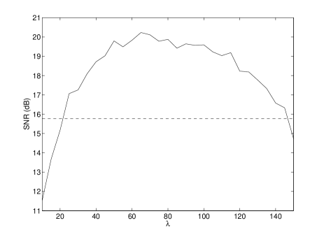
Fig. 2: Average Output SNR for different choices of $\lambda$ for $\sigma_{\mathrm{n}}$=0.05.

Fig. 3: $\lambda_{\mathrm{opt}}$ as a function of noise power ($\sigma_{\mathrm{n}}$). The continuous curve shows our approximation of $\lambda_{\mathrm{opt}}$.

As mentioned in the previous section, we expect an appropriate choice of $\lambda$ to be a decreasing function of $\sigma_{\mathrm{n}}$ since with the increase of noise power, the cost of approximation $({\bf A}{\bf x}\approx{\bf s})$ decreases. To verify this, for each value of $\sigma_{\mathrm{n}}$, we obtained the value of $\lambda_{\mathrm{opt}}$ using the curves similar to Fig. 2. Figure 3 shows the values of $\lambda_{\mathrm{opt}}$ as a function of $\sigma_{\mathrm{n}}$ in [0,0.15]. We fit these results with a curve of type $\frac{1}{\alpha+\beta x^{2}}$ to find the following rule of thumb for the choice of parameter $\lambda$:

$$\lambda\approx\frac{1}{0.007+3.5\sigma_{\mathrm{n}}^{2}}.$$ (10)

This formula gives a rough approximation for the choice of appropriate $\lambda$ in the initialization step of the algorithm.

Notice that we have two choices for the initialization of the proposed method: either to estimate $\sigma_{\mathrm{n}}$ directly from the observed mixtures [9] and then use (10) to find an approximation of $\lambda_{\mathrm{opt}}$, or to follow this iterative approach to solve the problem:

1. choose an arbitrary reasonable value of $\sigma_{\mathrm{n}}$.

2. take $\lambda_{\mathrm{opt}}$ from the curve.

3. run the algorithm and after convergence, compute an estimation of $\sigma_{\mathrm{n}}$ from the obtained source vector and then goto step 2.

Experiment 2. Speed and performance

In order to measure the speed of our algorithm, we run the algorithm 100 times for $m=1000$, $n=400$ and $\sigma_{\mathrm{n}}=0.05$. The simulation is performed in MATLAB7 environment using an Intel 2.8Ghz processor and 512MB of memory. The average run time of SL0DN was 2.062 seconds while the average time for SL0 was 0.242 seconds. Although SL0DN is somehow slower than SL0, but regarding to Table I in [8], the algorithm is still much faster than $\ell_{1}$-magic and FOCUSS.

We proceed with the performance analysis of the proposed algorithm. In this experiment, we fix the parameters $m,n,p$ with those of experiment 1 and for each value of $\sigma_{\mathrm{n}}$, choose the value of $\lambda$ with (10). In Fig. 4 the average output SNR is compared to the results of SL0. It can be seen that except for low-noise mixtures $(\sigma_{\mathrm{n}}<0.02)$, SL0DN achieves a better SNR. Thus for noisy mixtures, the case for most real data, the act of approximately satisfying ${\bf A}{\bf s}={\bf x}$ constraint is justified experimentally.

We also compared the results SL0DN with Basis Pursuit DeNoising (BPDN) which is much faster than BP. We used Gradient Projection for Sparse Reconstruction (GPSR) [10] algorithm for BPDN. The results of GPSR are shown in Fig. 4 with dotted line. As we see, the average SNR curve of GPSR lies under the two other curves except for low noise mixtures. It worths mentioning that the average run time of GPSR was 3.156 seconds.

Experiment 3. Dimension Dependency

In this experiment we study the performance of the proposed method for different dimensions of sources and mixtures. In this experiment, the values of $m$ and $n$ change within a constant ratio ($n=0.4m$). The average output SNR for both methods are shown in Fig.5. The results suggest that the quality of estimation is almost independent of the dimensions.

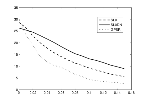
Fig. 4: Comparison between SL0DN, SL0 and BPDN.

Fig. 5: Average Output SNR versus $m$. Averages are taken over $100$ experiments.

5 conclusion

We presented a fast method for Sparse Component Analysis (SCA) or atomic decomposition on over-complete dictionaries, in presence of additive noise. The method was a generalization of SL0 method. The proposed method was based on smoothed $\ell^{0}$-norm
 minimization and satisfying the equality constraint approximately instead of exact equality constraint. The proposed method is fast while being more robust against noisy mixtures than the original SL0. Experimental results approved the performance and the noise-tolerance of our method for noisy mixtures.

References

- [1] A. Hyvärinen, J. Karhunen, and E. Oja, Independent Component Analysis, John Wiley & Sons, 2001.
- [2] S. Mallat and Z. Zhang, “Matching pursuits with time-frequency dictionaries,” IEEE Trans. on Signal Proc., vol. 41, no. 12, pp. 3397–3415, 1993.
- [3] D. L. Donoho, M. Elad, and V. Temlyakov, “Stable recovery of sparse overcomplete representations in the presence of noise,” IEEE Trans. Info. Theory, vol. 52, no. 1, pp. 6–18, Jan 2006.
- [4] R. Gribonval and S. Lesage, “A survey of sparse component analysis for blind source separation: principles, perspectives, and new challenges,” in Proceedings of ESANN’06, April 2006, pp. 323–330.
- [5] S. S. Chen, D. L. Donoho, and M. A. Saunders, “Atomic decomposition by basis pursuit,” SIAM Journal on Scientific Computing, vol. 20, no. 1, pp. 33–61, 1999.
- [6] D. L. Donoho, “For most large underdetermined systems of linear equations the minimal -norm solution is also the sparsest solution,” Tech. Rep., 2004.
- [7] E. Candes and J. Romberg, “-magic: Recovery of sparse signals via convex programming” 2005, URL: www.acm.caltech.edu/l1magic/downloads/l1magic.pdf.
- [8] G. H. Mohimani, M. Babaie-Zadeh, and C. Jutten, “Fast sparse representation based on smoothed -norm,” accepted for publication in IEEE Trans. on Signal Proc. (available as eprint arXiv 0809.2508).
- [9] H. Zayyani, M. Babaie-Zadeh and C. Jutten “Source estimation in noisy Sparse Component Analysis,” 15’th Intl. Conf. on Digital Signal Processing (DSP2007), pp. 219-222 July 2007.
- [10] Mario A.T. Figueiredo, Robert D. Nowak, and Stephen J. Wright, “Gradient projection for sparse reconstruction: Application to compressed sensing and other inverse problems”, IEEE Journal of Selected Topics in Signal Processing: Special Issue on Convex Optimization Methods for Signal Processing, 1(4), pp. 586-598, 2007