Three-dimensional numerical simulations of the pulsar magnetosphere: Preliminary results

We investigate the three-dimensional structure of the pulsar magnetosphere through time-dependent numerical simulations of a magnetic dipole that is set in rotation. We developed our own Eulerian finite difference time domain numerical solver of force-free electrodynamics and implemented the technique of non-reflecting and absorbing outer boundaries. This allows us to run our simulations for many stellar rotations, and thus claim with confidence that we have reached a steady state. A quasi-stationary corotating pattern is established, in agreement with previous numerical solutions. We discuss the prospects of our code for future high-resolution investigations of dissipation, particle acceleration, and temporal variability.

1 Introduction

In the 40 years following the discovery of pulsars, significant progress has been made towards understanding the pulsar phenomenon (e.g. Michel 1991; Bass et al. 2008). We know that pulsars are magnetized neutron stars with non-aligned rotation and magnetic axes (oblique rotators). We also know that pulsars lose rotational energy and spin down through electromagnetic torques due to large-scale electric currents in their magnetospheres.

Unfortunately, several pieces of the puzzle are still missing. In particular, we have only a vague idea about the structure of the pulsar magnetosphere. An analytic expression only exists for the structure of the magnetosphere of the vacuum rotator (the retarded dipole solution, Deutsch 1955), but real pulsars are certainly not in vacuum since electrons and positrons are copiously produced due to the high surface electric fields induced by rotation. Numerical solutions are hard to obtain because the magnetosphere develops singular current sheets, and the problem is fundamentally three-dimensional with an extended spatial dynamic range. Our current understanding is based on the axisymmetric solution obtained for the first time in Contopoulos, Kazanas & Fendt (1999) (hereafter CKF). This solution has since been confirmed, improved, and generalized by several other authors (e.g. Gruzinov 2005, Contopoulos 2005, Timokhin 2006, Komissarov 2006, McKinney 2006). The first time-dependent numerical simulations of the pulsar magnetosphere in 3D were performed by Spitkovsky (2006).

Our current understanding suggests that the general 3D magnetosphere consists of regions of closed and open field lines (those that are stretched out to infinity away from their point of origin on the surface of the neutron star). It also suggests that a large-scale electric current circuit is established along open magnetic field lines. In that picture, electric current closure is guaranteed through a current sheet that flows in the equatorial region and along the boundary between open and closed field lines. The equatorial current sheet is confined between latitudes $\pm\theta$ above and below the rotation equator ($\theta$ being the inclination angle between the rotation and magnetic axes) and has an undulating shape of a spiral form with radial wavelength equal to $2\pi$ times the light cylinder distance $r_{lc}\equiv c/\Omega_{*}$, where $\Omega_{*}$ is the angular velocity of rotation of the central neutron star (e.g. Bogovalov 1999). A large-scale pattern of electromagnetic energy flow (Poynting flux) and charged relativistic particle wind is established along open field lines. The details of how the particles are supplied are not understood well. Moreover, the equatorial current sheet is probably unstable, and may not survive beyond the light cylinder (Romanova, Chulsky & Lovelace 2005). This is different from the stable heliospheric equatorial current sheet that is simply the tangential discontinuity convected with the velocity of the solar wind plasma (Landau & Lifshitz 1969).

The details of the 3D solution are of paramount importance for answering several questions about the pulsar phenomenon such as where in the magnetosphere the observed electromagnetic radiation is coming from, what determines the radiation spectrum and the pulse profile, what accelerates the pulsar wind, etc. Guided by our experience from the solution of the steady-state axisymmetric problem, we believe that a promising approach to obtaining the structure of the 3D pulsar magnetosphere may be through time dependent relativistic ideal MHD numerical simulations of a rotating magnetized star which, when run long enough, will hopefully relax to the steady-state solution.

The pulsar magnetosphere problem belongs to a subclass of relativistic MHD, that of Force-Free Electrodynamics, hereafter FFE (e.g. Gruzinov 1999). FFE assumes that the relativistic medium is on the one hand dense enough to provide charge carriers that will guarantee ‘infinite’ plasma conductivity and therefore

$${\bf E}\cdot{\bf B}=0\ \mbox{everywhere,}$$ (1)

and on the other hand tenuous enough for plasma inertia and pressure terms to be neglected and therefore

$$\rho_{e}{\bf E}+{\bf J}\times{\bf B}=0\ \mbox{everywhere.}$$ (2)

Here,

$$\rho_{e}\equiv\frac{1}{4\pi}\nabla\cdot{\bf E}$$ (3)

is the charge density distributed in space, and ${\bf J}$ is the electric current. The pulsar magnetosphere is a unique physical system in which the above conditions are satisfied over its largest part. Deviations from FFE do exist in singular regions of the magnetosphere, and these introduce important physical complications to the problem.

As we said above, the first FFE numerical simulations of the 3D pulsar magnetosphere were performed by Spitkovsky (2006). Our main concern with those simulations has been that they run only for a limited amount of time which may not have been enough to reach steady state (see § 2). Since no equivalent numerical simulations existed up to now in the literature, we have tried to reproduce Spitkovsky’s conclusions based on our experience from two idealized cases where we know the solution almost analytically (Contopoulos 2007), but without success. In view of the above, and because of the central role understanding the structure of the pulsar magnetosphere plays for pulsar research, we decided to independently develop our own Finite-Difference Time-Domain (hereafter FDTD; Taflove & Hagness 2005) FFE code. The new element is that we have now implemented the technique of Perfectly Matched Layer (hereafter PML; Berenger 1994, 1996) which is quite efficient in minimizing reflection and maximizing absorbtion from the outer boundaries of the simulation box. Such boundary conditions imitate open space, allowing thus to run our simulations for very long times up to satisfactory numerical convergence to a steady state. As we will see below, we are currently in a position to address the same problem, in comparable detail, using just a standard off-the-shelf PC.

In § 2 we justify our effort to implement PML outer boundary conditions by laying out our criticism of existing numerical results. In § 3, we describe the computer code that we have developed and the solutions to the numerical problems that we encountered when running our simulations. Our first results and discoveries with detail comparable to existing numerical simulations are presented in § 4. We conclude in § 5 with a discussion on numerical convergence and tests, as well as a short presentation of future prospects for our code.

2 Need for longer numerical simulations

We will assume that relativistic ideal MHD, and in particular its Force-Free idealization is a valid description of the pulsar magnetosphere (we will get back to the issue of non-ideal processes in § 5). Therefore, the magnetospheric electric and magnetic fields ${\bf E}$ and ${\bf B}$ satisfy not only Maxwell’s equations

$$\frac{\partial{\bf E}}{\partial t}=c\nabla\times{\bf B}-4\pi{\bf J}\ ,$$ (4)

$$\frac{\partial{\bf B}}{\partial t}=-c\nabla\times{\bf E}\ ,\ \mbox{and}$$ (5)

$$\nabla\cdot{\bf B}=0\ ,$$ (6)

but also eqs. (1) and (2). After some algebra, we obtain

$${\bf J}=\rho_{e}c\frac{{\bf E}\times{\bf B}}{B^{2}}+\frac{c}{4\pi}\frac{({\bf B}\cdot\nabla\times{\bf B}-{\bf E}\cdot\nabla\times{\bf E})}{B^{2}}{\bf B}$$ (7)

(Gruzinov 1999, 2005). Here, $c{\bf E}\times{\bf B}/B^{2}$ is the pulsar wind drift velocity. As we will see in the next section, a stationary corotating pattern is established in the pulsar magnetosphere, where the electric field is given by

$${\bf E}=-\frac{1}{c}({\bf\Omega}_{*}\times{\bf r})\times{\bf B}$$ (8)

(e.g. Muslimov & Harding 2005).

If one starts with a magnetic field configuration ‘anchored’ onto the rotating magnetized neutron star (e.g. a simple magnetostatic dipole), and if one sets the star in rotation, electric currents will develop which will populate the magnetosphere with electric charge originating in the stellar surface. It is natural to expect that if one integrates eqs. (4) and (5) long enough, the magnetosphere will relax to the final steady state, if such a steady state indeed exists. This will determine the distribution of electric charge, electric current, electromagnetic energy flow (Poynting flux), and pulsar wind drift velocities in the pulsar magnetosphere.

As we said, there are some important complications in this approach. The first one is that as the simulation evolves, current sheets appear where ${\bf J}$ becomes formally infinite and FFE breaks down. In the equatorial current sheet, the magnetic field goes to zero. At those positions, the electric field risks becoming greater than the magnetic field, and the drift velocity risks becoming greater than the speed of light. Physically, this corresponds to runaway particle acceleration (we will come back to this point in § 5), therefore, some way of restricting drift velocities to subluminal values must be incorporated in the code. The second complication is the fundamental 3D nature of the problem. In order to treat both the smallest (current sheets, neutron star polar cap) and largest physical scales of the system (light cylinder, equatorial current sheet undulations), one needs a numerical simulation with sufficient spatial dynamic range. The simulation must run long enough to reach convergence and come up with a believable solution. Without the implementation of non-reflecting and absorbing outer boundaries, simulation runs are limited by the time it takes for the transient wave that results from the initiation of the central neutron star rotation to reach the outer boundary of the simulation and return to affect the region of interest. It is precisely this complication that limits current state of the art computer simulations to less than about 2 central neutron star rotations, and the region of believable results not much further than about 2 light cylinder radii. We are, therefore, convinced that a promising approach to making significant progress is to run the simulations for much longer timescales by implementing non-reflecting and absorbing outer boundaries in the code.

Another interesting issue has to do with the pulsar spindown rate $L$ as a function of the inclination angle $\theta$ as obtained by Spitkovsky (2006), namely

$$L(\theta)=\frac{B_{*}^{2}r_{*}^{6}\Omega_{*}^{4}}{4c^{3}}(1+\sin^{2}\theta)\ ,$$ (9)

where $B_{*}$, $r_{*}$ are the polar dipole magnetic field and radius of the central neutron star respectively. Most people are content with the approximation that pulsars spin down at the same rate as $90^{o}$ vacuum dipole rotators, namely that $L(\theta)\approx B_{*}^{2}r_{*}^{6}\Omega_{*}^{4}/(6c^{3})$; however, this is not accurate, since the dependence of $L$ on the magnetic inclination angle $\theta$ has important implications for the evolution and distribution of pulsars in the $P-\dot{P}$ diagram (Contopoulos & Spitkovsky 2006). We would like to independently confirm eq. 9 with our own numerical code.

3 FFE with central symmetry and PML outer boundaries

In order to solve the system of eqs. (4) and (5) we implemented the FDTD Yee algorithm (Yee 1966). According to this, electric field components are defined parallel to the mesh cell sides, whereas magnetic field components are defined perpendicular to mesh cell faces. Apparently, this staggered mesh configuration guarantees low numerical diffusivity, something that is required in electrodynamic problems with sharp gradients such as the one we are presently addressing. The field components required at other mesh positions are obtained by first-order interpolation. We decided to implement a cartesian numerical grid $(x,y,z)=(i\delta,j\delta,k\delta)$ (where $i,j,k$ are integers and $\delta$ is the grid spatial resolution) rather than a cylindrical or spherical numerical one in order not to have to deal with numerical problems around the rotation axis. Moreover, instead of the staggered leapfrog time integration for the electric and magnetic field components of the original Yee algorithm, we chose to use third-order Runge-Kutta for the time integration. This approach is more accurate and provides both the electric and magnetic field at the same time moments. Finally, because of the special nature of the pulsar magnetosphere problem, we implemented central symmetry in order to reduce computer memory requiremens by one half (we solve only for $x\geq 0$, and set ${\bf B}(x=0^{-},y,z)={\bf B}(x=0^{+},-y,-z)$, and ${\bf E}(x=0^{-},y,z)=-{\bf E}(x=0^{+},-y,-z)$). Another one half of computer memory is saved when we integrate our equations in a sphere and not in a cube centered around the neutron star. What we mean is that, in an integration cube of size $L^{3}$, electromagnetic fields at the corners remain unchanged before the spherical wave initiated by the onset of stellar rotation (see below) reaches the surface of the cube. There is, therefore, no need to reserve computer memory for the cube’s corners, and with proper indexing of the rectangular grid cells, we may integrate our equations on only the cells interior to radius $L/2$. However, PML outer boundaries can only be implemented on planar surfaces, therefore, we had to return to integrating in a cube.

The electric current term in eq. (4) is introduced similarly to Spitkovsky (2006). Instead of calculating both terms in eq. (7), we use only the term perpendicular to the magnetic field (the first one) to update the electric field, and ignore the term parallel to it. The magnetic field is updated through eq. (5). The electric field thus obtained will have a component parallel to the magnetic field and a component perpendicular to it. In accordance to eq. (1), the second component would be ‘killed’ by the term in the electric current that we left out. We instead ‘kill’ this term ourselves and thus impose the verticality condition (eq. 1). At the same time we need to secure that the drift velocity remains everywhere subluminal. We impose this restriction by rescaling (after each time step) the electric field wherever the condition $E\leq B$ is violated. The problem is that electric and magnetic field components are defined at different grid positions, and the above conditions are implemented using first order interpolation between neighboring grid positions. After each update of the electric field components the two conditions are only approximately satisfied. We found that the updated electric field remains almost unchanged after imposing the verticality and rescaling conditions three times in a row. The benefit of this approach is that it may be generalized to the physical case where eq. 1 breaks down in certain parts of the magnetosphere when a component of the electric field parallel to the magnetic field is allowed to develop (see § 5).

As we said in the previous section, we insisted on the implementation of PML outer boundaries in order to be able to run our simulations long enough to claim with confidence that we’ve reached a steady state. A detailed description of the PML formulation can be found in Berenger (1996), Taflove & Hagness (2005) (see Appendix). The boundary layers extend beyond the outer surfaces of our integration cube around the central neutron star. We found that PML with 10-20 grid zones absorb very efficiently transient electromagnetic disturbances that originate in the integration domain without reflecting them back. Inside the PML zone we have chosen a cubic profile for the absorption coefficient $\sigma$. A careful choice for the maximum value of $\sigma$ is important mostly in the cases of high values of the inclination angle $\theta$.

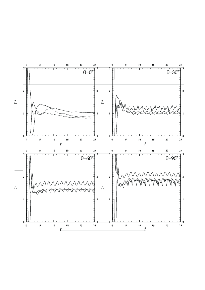
Figure 1: Total Poynting flux $L$ crossing 3 cubes with sides 0.64, 2, and 3 times $r_{lc}$ centred around the rotating neutron star as a function of time $t$ for various values of the inclination angle $\theta$ (top to bottom curves in each sub-panel respectively). $L$ in units of the CKF canonical luminosity (eq. 9 for $\theta=0^{\circ}$). $t$ in units of the light cylinder crossing time $r_{lc}/c$ (one period of rotation is equal to $2\pi$). The small oscillations seen at inclinations $\theta\neq 0^{o}$ are an artifact of our cartesian numerical grid and do not represent real magnetospheric oscillations (see text for details).

The problem that we solve is simple. We consider a spherical star extending out to radius $r_{*}$. We start at $t=0$ with a dipole magnetic field ${\bf B}_{\rm dipole}({\bf r};\theta)$ at an angle $\theta$ with respect to some rotation axis direction. In most of our simulations, we took the rotation axis to coincide with the $z$-axis of our cartesian grid, but in principle, it can be arbitrary. ${\bf E}=0$ everywhere. At $t=0^{+}$ we initiate the rotation of the central star with angular velocity $\Omega_{*}$ as follows: at all fixed grid points inside $r_{*}$ and at each time step, we update the magnetic field with that corresponding to an inclined dipole in rotation around the given axis direction ${\bf B}_{\rm dipole}({\bf r},t;\theta)$, and introduce a non-zero electric field according to eq. 8. We solve the set of equations that we presented in the previous section only on grid points that lie outside $r_{*}$. Note that the smaller (larger) $r_{*}$ is the more (less) physical our simulation (in a real pulsar, $r_{*}/r_{lc}\leq 10^{-3}$). On the other hand, high (low) values of $r_{*}$ provide a better (worse) description of the star in a cartesian grid. We noticed that when $\theta=0^{o}$ the solution is more insensitive to the chosen value of $r_{*}$, while for higher values of $\theta$ lower values of $r_{*}$ are needed in order to get a better description of the rotating magnetosphere. Taking the above into account we adopted the value $r_{*}=0.2r_{lc}$.

4 A dynamic magnetosphere

With the implementation of PML outer boundaries and central symmetry, we were able to run our simulations for several neutron star rotations over a cubic spatial grid centered on the neutron star with sides 4.8 times $r_{lc}$ and spatial resolution $\delta=0.04r_{lc}$ on an Intel Core 2 Duo E6600 2 Gbyte RAM standard off-the-shelf PC. Such simulations have spatial resolution comparable to that of existing ones (Spitkovsky 2006), only now we are able to run them for much longer times.

In Fig. 1 we plot the total Poynting flux calculated over a series of cubes centered on the neutron star with sides 0.64, 2, and 3 times $r_{lc}$ respectively as a function of time. The 3 curves are clearly displaced horizontally between them by the amount of time it takes for the initial spherical wave induced by the onset of the stellar rotation to cross each subsequent calculation cube. We observe that the further away from the central star the calculation cube is, the smaller the estimated Poynting flux. For an ideal dissipationless calculation in steady state, the same amount of electromagnetic energy that leaves the star in every period of stellar rotation would cross all of the above cubes, and the position and shape of the surfaces over which we calculate the Poynting flux would not matter. In a real calculation like the present one, though, some amount of electromagnetic energy is lost between the cubes due to numerical dissipation. In the non-axisymmetric case, this is expected to yield periodic oscillations in the Poynting flux computed over the above cubes at one quarter of the period of the star, which do not represent real magnetospheric oscillations. An additional artificial source of periodicity in the non-axisymmetric cases comes from the fact that the representation of the rotating stellar field on the cartesian grid repeats itself every quarter of a period. The amplitude of these oscillations is smaller than about $10\%$, and therefore, Fig. 1 is a test of both the convergence and accuracy of our calculations.

In the axisymmetric case the simulation converges after about 2.5 stellar rotations ($t\geq 15$ in units of the light cylinder crossing time $r_{lc}/c$). This justifies our insistence on implementing PML outer boundaries. We repeated our calculation for $\theta=30^{\circ},60^{\circ}$ and $90^{\circ}$, and at those inclinations, the simulation converges in about 1 stellar rotation. The final axisymmetric quasi-stationary steady state is practically indistinguishable from the CKF steady state (see discussion below). The further away the Poynting flux is estimated numerically, the lower its value. Therefore, in order to estimate the true stellar energy loss rate, we computed the Poynting flux as close to the central star as possible, on a cube with side equal to $0.64r_{lc}$ centred around it (that is only 3 grid zones away from the surface of the star). Our results are consistent with eq. (9) (within $5\%$), which constitutes an independent confirmation of the results of Spitkovsky (2006). The numerical energy losses are at most on the order of 15% at all inclinations, and they occur mostly inside the light cylinder.

A practical problem with the general 3D case is the visualization of the magnetic field configuration. In axisymmetry, we define magnetic flux surfaces as surfaces of revolution of magnetic field lines around the magnetic and rotation axis. We may thus plot the cross sections of magnetic flux surfaces with the meridional plane.

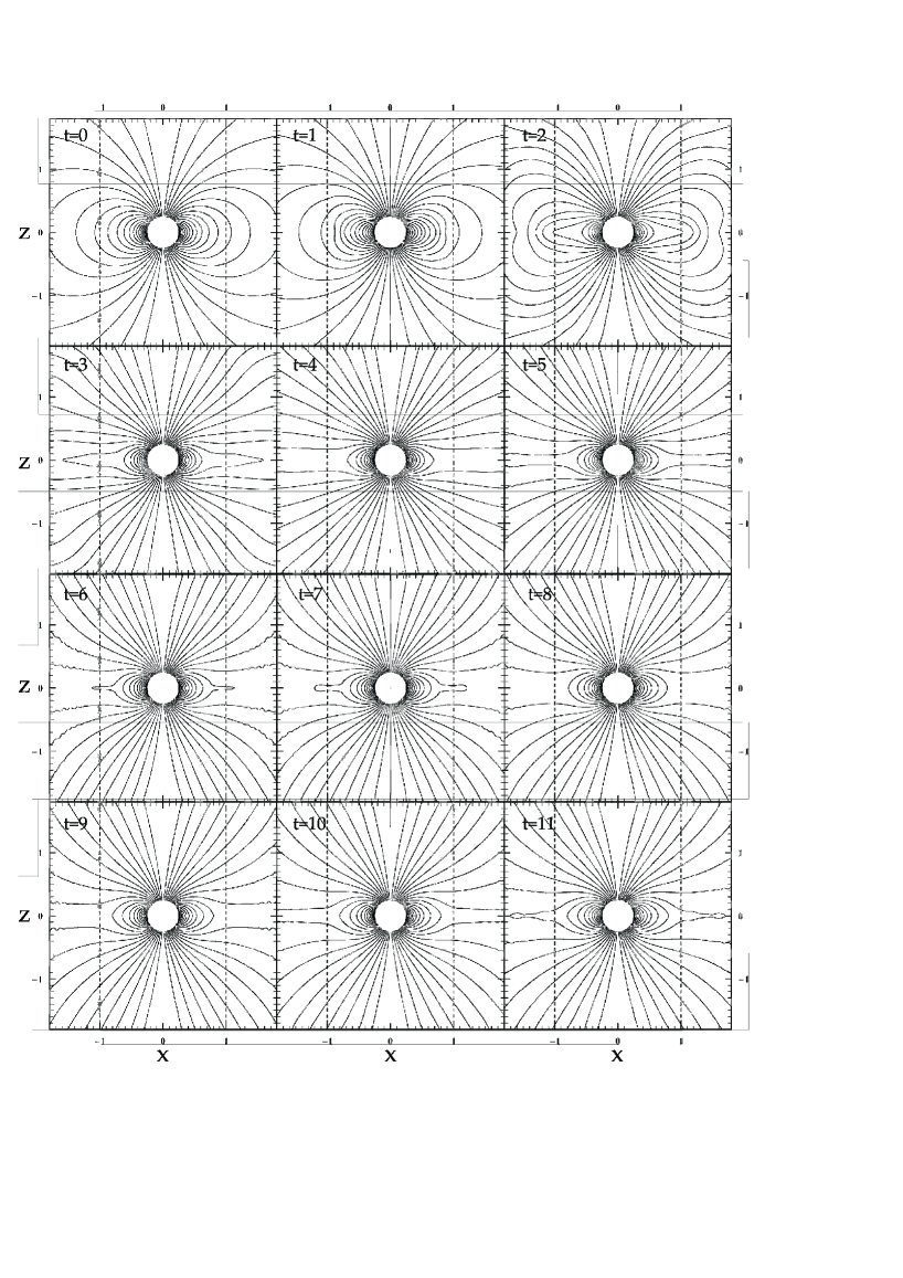
Figure 2: Time sequence of magnetic flux surfaces along the meridional plane $(x,z)$ for an aligned rotator ($\theta=0^{\circ}$). Distances in units of $r_{lc}$. Times $t$ in units of $r_{lc}/c$. Initial state at upper left. Light cylinder shown with dashed line.

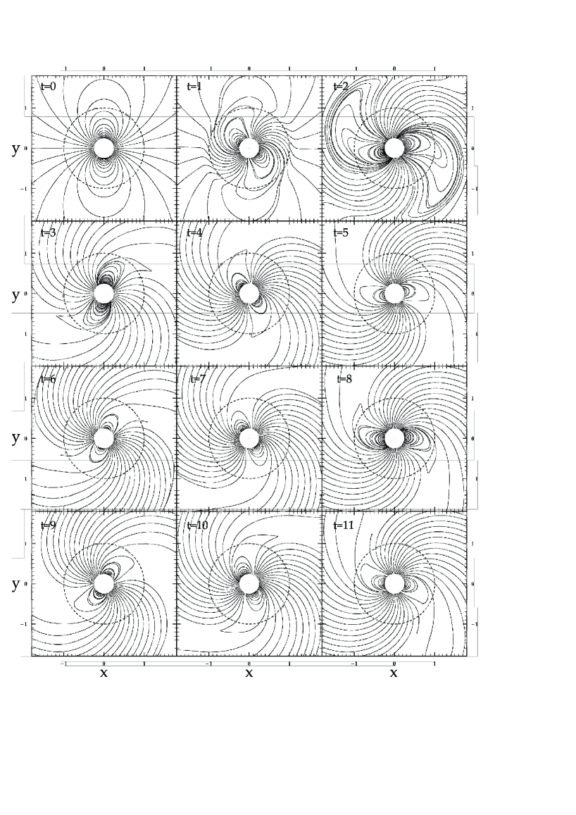
Figure 3: Time sequence of equatorial field lines originating on the surface of the star for a $\theta=90^{\circ}$ oblique rotator. Units as in Fig. 2. Initial state at upper left. Light cylinder shown with dashed line.

In the general 3D case, the choice of flux surfaces is not unique, since any closed line along the surface of the neutron star traces a certain flux surface along which field lines flow. When $0^{\circ}<\theta<90^{\circ}$, the only way to visualize the solution is by the direct drawing of 3D magnetic field lines, and plane cuts through the magnetosphere do not mean much. When $\theta=90^{\circ}$, though, magnetic field lines originating on the equatorial plane stay on that plane (because of symmetry), and therefore visualization of that particular case is straightforward.

In Fig. 2, we show a time sequence of the approach to steady state when $\theta=0^{\circ}$ by plotting the cuts of axisymmetric magnetic flux surfaces with the meridional plane $(x,z)$. The light cylinder is denoted with dashed lines. We see that an initial wave travels out at the speed of light ‘informing’ the magnetosphere that the star is set in rotation at $t=0$. Behind this wave, formerly dipolar magnetic field lines are stretched in the radial direction, and are also twisted in the direction opposite to the stellar rotation (‘backwards’). An equivalent way to understand this is that electric currents develop behind this wave which carry along electric charges. These are the ones that will populate the pulsar magnetosphere with the space-charge density required by the steady-state solution. In steady state, field lines that close inside the light cylinder cannot and indeed do not contain electric currents (because of North-South symmetry). Beyond the light cylinder, formerly closed field lines are stretched out to infinity. It is interesting to notice that, very quickly (within about half a rotation), a large fraction of formerly closed field lines open up, and the closed line region ends at about $80\%$ of the light cylinder distance $r_{lc}$. This effect manifests itself in the evolution of the total Poynting flux through our inner calculation cube, where $L(0^{\circ})$ reaches a value of about 1.5 times its final steady-state value. Beyond that point, the final steady state is gradually approached within about 2.5 stellar rotations, as the tip of the closed line region slowly approaches the light cylinder through a sequence of equatorial reconnection and plasmoid generation events. Every time a plasmoid is detached, the tip and the whole magnetosphere relax and try to readjust from the stretching. The process repeats itself again and again, and never actually disappears completely. The origin of this effect is magnetic diffusivity, which in our case is entirely due to numerical dissipation. Note that a similar behavior was observed in the very high resolution 2D simulations of Spitkovsky (2006) where it took him about 20 stellar rotations to reach the final steady state. Higher resolution simulations with adaptive mesh refinement are needed to better capture this effect in 3D. In Fig. 4 we plot the magnitude of the magnetic field on the equator (in units of $B_{*}(r_{*}/r_{lc})^{3}/2$) at two different times during the approach to steady state (compare with fig. 11 of Timokhin 2006 and fig. 1 of Spitkovsky 2006).

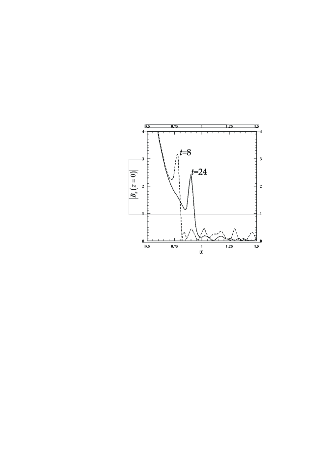
Figure 4: The magnitude of the magnetic field on the equator (in units of $B_{*}(r_{*}/r_{lc})^{3}/2$) at two different times during the approach to steady state when $\theta=0^{\circ}$.

After testing our code against the well understood axisymmetric case, we proceeded with confidence to the study of nonzero values of the inclination angle $\theta$. In Fig. 3 we show a time sequence of the approach to steady state when $\theta=90^{\circ}$ by plotting magnetic field lines that originate on the surface of the star in the equatorial plane $(x,y)$. The non-vacuum solution is different from the vacuum one in that magnetic field lines cannot close beyond the light cylinder (closed field lines impose corotation with the central star). As in the axisymmetric case described above, after the passage of an initial transient wave, the magnetosphere is populated with electric charges due to electric currents. The approach towards steady state is similar to the axisymmetric one but takes only about one stellar period. Plasmoid generation from the tip of the closed line region is also observed. Overall, our results are in qualitative agreement with the results of Spitkovsky (2006).

5 Discussion

We have shown that the implementation of PML outer boundary conditions allows us to perform reliable time-dependent simulations of the 3D pulsar magnetosphere on a spatial numerical grid extending only a small distance beyond the light cylinder. Some amount of empirical adjustment of the PML parameters is needed. We found that a PML boundary thicker than 10 grid zones seems to work satisfactorily. As we described above, we tested our code against the well understood axisymmetric solution. We were also able to reproduce the vacuum solution. We confirmed that our conclusions are independent of the rotation axis orientation with respect to the grid orientation by performing test runs with the axis of rotation along various directions (e.g. along the simulation cube diagonal $(1,1,\sqrt{2})$). The grid resolution affects the spatial resolution and the numerical dissipation of our simulations. We performed simulations with $d=0.08r_{lc}$ and obtained comparable final steady states. A smaller $d$ allows us to implement a smaller central star. Numerical dissipation affects the details of the time evolution. In particular, when $\theta=0^{\circ}$, the approach to steady state takes around 2.5 stellar rotations when $d=0.04r_{lc}$, and around 1 stellar rotation when $d=0.08$. Moreover, plasmoids are generated about once every period when $d=0.04r_{lc}$ and about every one third of a period when $d=0.08r_{lc}$.

We end the present paper with a short discussion of the future prospects for our code. A very promising avenue for research would be to introduce physical prescriptions for the breakdown of ideal FFE in our code. This will be implemented as follows: we will relax the ideal MHD condition eq. (1), and instead of ‘killing’ the component of the electric field that is parallel to the magnetic field as described in § 3 above, allow for a nonzero parallel component as current emission models imply (e.g. Arons 1983; Daugherty & Harding 1982; Muslimov & Harding 2003; Cheng, Ho & Ruderman 1986; Romani 1996). We will thus be able to determine self-consistently the regions where dissipation of electromagnetic energy takes place in the framework of a particular high-energy emission model and thus check the validity of that model (e.g. inner, slot, or outer gap). We will also be able to identify the sources of plasma supply needed to make the force-free model viable in the first place. Another interesting feature of the pulsar phenomenon is its rich random non-periodic time variability often referred to as ‘timing noise’. It is natural for us to associate some of this variability with the continuous plasmoid generation at the tip of the closed line region. In a real pulsar, the situation is even more complicated since there is no final steady state to be reached because the light cylinder continuously moves out as the central star loses energy and spins down. In order to address the above issues, we are currently modifying our code to run in MPI parallel form with a much higher spatial resolution and spatial extent.

Appendix A Perfectly Matched Layer (PML) formulation

The PML method consists of adding a PML medium around the main computational domain where all the components of the electromagnetic field are split into two parts. This means that the 6 regular components $(E_{x},E_{y},E_{z},B_{x},B_{y},B_{z})$ integrated in the main computational domain yield 12 subcomponents $(E_{xy},E_{xz},E_{yx},E_{yz},E_{zx},E_{zy},B_{xy},B_{xz},B_{yx},B_{yz},B_{zx},B_{zy})$ inside the PML which are integrated according to the following set of equations (Berenger 1996):

$$\frac{\partial E_{xy}}{\partial t}+\sigma_{y}^{e}E_{xy} = \frac{\partial(B_{zx}+B_{zy})}{\partial y}$$ (10)

$$\frac{\partial E_{xz}}{\partial t}+\sigma_{z}^{e}E_{xz} = -\frac{\partial(B_{yz}+B_{yx})}{\partial z}$$ (11)

$$\frac{\partial E_{yz}}{\partial t}+\sigma_{z}^{e}E_{yz} = \frac{\partial(B_{xy}+B_{xz})}{\partial z}$$ (12)

$$\frac{\partial E_{yx}}{\partial t}+\sigma_{x}^{e}E_{yx} = -\frac{\partial(B_{zx}+B_{zy})}{\partial x}$$ (13)

$$\frac{\partial E_{zx}}{\partial t}+\sigma_{x}^{e}E_{zx} = \frac{\partial(B_{yz}+B_{yx})}{\partial x}$$ (14)

$$\frac{\partial E_{zy}}{\partial t}+\sigma_{y}^{e}E_{zy} = -\frac{\partial(B_{xy}+B_{xz})}{\partial y}$$ (15)

$$\frac{\partial B_{xy}}{\partial t}+\sigma_{y}^{b}B_{xy} = -\frac{\partial(E_{zx}+E_{zy})}{\partial y}$$ (16)

$$\frac{\partial B_{xz}}{\partial t}+\sigma_{z}^{b}B_{xz} = \frac{\partial(E_{yz}+E_{yx})}{\partial z}$$ (17)

$$\frac{\partial B_{yz}}{\partial t}+\sigma_{z}^{b}B_{yz} = -\frac{\partial(E_{xy}+E_{xz})}{\partial z}$$ (18)

$$\frac{\partial B_{yx}}{\partial t}+\sigma_{x}^{b}B_{yx} = \frac{\partial(E_{zx}+E_{zy})}{\partial x}$$ (19)

$$\frac{\partial B_{zx}}{\partial t}+\sigma_{x}^{b}B_{zx} = -\frac{\partial(E_{yz}+E_{yx})}{\partial x}$$ (20)

$$\frac{\partial B_{zy}}{\partial t}+\sigma_{y}^{b}B_{zy} = \frac{\partial(E_{xy}+E_{xz})}{\partial y}\ ,$$ (21)

where the conductivities $(\sigma_{x}^{e},\sigma_{y}^{e},\sigma_{z}^{e})$ and $(\sigma_{x}^{b},\sigma_{y}^{b},\sigma_{z}^{b})$ are defined below. When these parameters are set to zero we obtain Maxwell’s equations in vacuum. Note that each (total) field component inside the PML is calculated by adding its two subcomponents (e.g. $B_{x}=B_{xy}+B_{xz}$). At $t=0$, each subcomponent is set equal to one half the value of its corresponding field component.

Without loss of generality, we assume that the main computational domain is a cube with side $L$ centered around the origin of our cartesian coordinate system. In that case the PML technique requires that, inside the PML,

$$\sigma_{x}^{a} = 0\ \mbox{wherever}\ |x|<L/2,|y|>L/2,|z|>L/2$$ (22)

$$\sigma_{y}^{a} = 0\ \mbox{wherever}\ |x|>L/2,|y|<L/2,|z|>L/2$$ (23)

$$\sigma_{z}^{a} = 0\ \mbox{wherever}\ |x|>L/2,|y|>L/2,|z|<L/2\ ,$$ (24)

where, $a=(e,b)$. Theoretically, in the remaining PML regions the conductivities may have constant values. In practice, the finiteness of the grid resolution introduces artificial reflections at the interface between the PML and the main computational domain. For that reason it is more convenient to consider a less discontinuous transition along the directions the conductivities are nonzero. We have adopted the following cubic law for the variation of the conductivities,

$$\sigma_{i}^{a}\approx\sigma_{max}\left(\frac{d}{D}\right)^{3}\ ,$$ (25)

where, $d$ is the distance from the main cube, $D$ is the PML thickness, and $i=(x,y,z)$. Our simulations run with $D\sim 0.4-0.8$ length units and $\sigma_{,max}\sim 100-200$ inverse time units. These values seem to work satisfactorily in both the vacuum and non-vacuum cases.