Boosting the Accuracy of Finite Difference Schemes via Optimal Time Step Selection and Non-Iterative Defect Correction

Abstract

In this article, we present a simple technique for boosting the order of accuracy of finite difference schemes for time dependent partial differential equations by optimally selecting the time step used to advance the numerical solution and adding defect correction terms in a non-iterative manner. The power of the technique is its ability to extract as much accuracy as possible from existing finite difference schemes with minimal additional effort. Through straightforward numerical analysis arguments, we explain the origin of the boost in accuracy and estimate the computational cost of the resulting numerical method. We demonstrate the utility of optimal time step (OTS) selection combined with non-iterative defect correction (NIDC) on several different types of finite difference schemes for a wide array of classical linear and semilinear PDEs in one and more space dimensions on both regular and irregular domains.

 

 

1 Introduction

High-order numerical methods for partial differential equations (PDEs) will always be valuable for increasing the computational efficiency of numerical simulations. Thus, it is not at all surprising that a great deal of effort in numerical PDEs continues to be focused on the development of high-order numerical schemes [1, 2, 3, 4, 5, 6, 7]. Typically, high-order accuracy is achieved by constructing schemes that are formally high-order accurate. However, high-order accuracy can also be obtained by using formally low-order schemes in clever ways (e.g. Richardson extrapolation and compact finite difference schemes [1]). When possible, the latter approach can be a powerful way to boost the accuracy of a numerical method without introducing too much additional algorithmic (and programming) complexity.

Optimization of numerical parameters (e.g. $\Delta x$ and $\Delta t$) is an important, but relatively uncommon, approach for maximizing the accuracy of numerical schemes. Often, all combinations of numerical parameters are considered equally good. For some problems, however, optimizing the numerical parameters can significantly increase the accuracy of the numerical solution. For example, the well-known unit CFL condition, $\Delta t=\Delta x/a$, for the first-order upwind forward Euler discretization of the linear advection equation completely eliminates the numerical error introduced by the scheme [8]. Another well-known example is the boost in the order of accuracy that results from setting the time step to $\Delta t=\Delta x^{2}/6D$ when the 1D diffusion equation is solved using forward Euler time integration with the standard second-order central difference approximation for the Laplacian. As a final example, Zhao showed that an appropriate choice of the weight factor $\theta$ in the theta-method can significantly decrease the error in finite element solutions to the diffusion equation [9].

In this article, we present a simple technique for boosting the order of accuracy of finite difference schemes for time dependent PDEs by optimally choosing the time step and, when necessary, adding defect correction terms in a non-iterative manner. This technique is a systematic generalization of the ideas underlying some of the examples mentioned above. Optimal time step (OTS) selection is based on the observation that a carefully chosen time step can simultaneously eliminate low-order terms in both the spatial and temporal the discretization errors. It combines the well-known approach of using knowledge of the structure of the PDE to reduce numerical error with the less-common notion that an optimal choice of numerical parameters can boost the effectiveness of algorithmically simple and computationally low-cost numerical schemes. For some problems, OTS alone is sufficient to allow a formally low-order method to deliver high-order accuracy. However, addition of defect correction terms is generally required to eliminate residual terms in the leading-order truncation error. It is important to emphasize that, unlike traditional defect/deferred correction methods [10, 11, 12, 13, 14] which use defect correction terms to iteratively refine the solution at each time step, we take a non-iterative defect correction (NIDC) approach that incorporates defect correction terms directly into the original finite difference scheme.

As a technique for enhancing numerical methods, OTS-NIDC has several desirable features. Like any technique that leads to high-order methods, OTS-NIDC produces schemes that greatly reduce the computational cost required to obtain a numerical solution of a desired accuracy. However, its real power comes from the fact that it achieves high-order accuracy while being based solely on very simple, formally low-order finite difference schemes. In other words, OTS-NIDC allows us to extract as much accuracy as possible from an existing numerical scheme with minimal additional work. For instance, we will see how OTS-NIDC makes it possible to achieve 4th-order accuracy for the diffusion equation in any number of space dimensions using only a second-order stencil for the Laplacian and explicit time integration. Moreover, high-order accuracy is not restricted to problems on simple, rectangular domains; irregular domains are straightforward to handle by appropriately setting the values in ghost cells [3, 4, 15, 16]. OTS-NIDC is even beneficial when using finite difference schemes to solve some nonlinear PDEs. While there are certainly limitations to OTS-NIDC, we will see that there are many problems where it is useful.

This article is organized as follows. In the remainder of this section, we compare OTS-NIDC to a few related numerical techniques. In Section 2, we present the theoretical foundations of OTS-NIDC and show how it boosts the order of accuracy for formally low-order numerical schemes. In Section 3, we demonstrate the utility of OTS-NIDC to problems in one space dimension by applying it to finite difference schemes for several classical linear and nonlinear PDEs. In Section 4, we show that OTS-NIDC is useful for problems in multiple space dimensions by applying it the 2D linear advection equation and the 2D diffusion equation. To illustrate the ease with which high-order accuracy can be achieved for problems on arbitrary domains, the 2D diffusion equation is solved on both regular and irregular domains. For each PDE in Sections 3 and 4, we provide the numerical analysis required to calculate the optimal time step size, the defect correction terms, and the order of accuracy. Finally, we offer some concluding remarks in Section 5.

1.1 Comparison with Traditional Defect/Deferred Correction Methods

Defect/deferred correction is a well-known strategy for boosting the order of accuracy of finite difference schemes for time dependent PDEs. It usually takes one of two forms: (1) iterative refinement of the numerical solution [10, 11, 12, 13, 14] or (2) derivation of high-order compact schemes for the spatial derivative operator treating time derivatives as source terms [1, 4, 6].

For iterated defect/deferred correction, the numerical solution at each time step is computed by iteratively adding correction terms that are calculated from lower accuracy iterates. When used to improve the temporal order of accuracy, the iterative approach can help to ensure stability of the time integration scheme [14]. Although there are instances where iterative defect correction has been used to eliminate both spatial and temporal errors [12], it is usually used to improve only one of these errors [10, 13, 14]. Note that unlike iterated defect correction, OTS-NIDC requires no iteration during each time step because it computes correction terms using only the solution at the previous time step(s) (as opposed to requiring an estimate of the solution at the current time).

High-order compact schemes focus on eliminating spatial discretization errors when deriving the semi-discrete equations. When applied to time dependent PDEs, a high-order compact scheme for the spatial derivative operator is derived treating time derivatives as source terms [1, 4, 6]. After deriving the high-order spatial discretization, any time differencing scheme may be applied to discretize the time derivatives. While this approach is very general, it really only provides a mechanism for reducing spatial discretization error. Temporal discretization errors are completely controlled by the choice of time differencing scheme. Note that because high-order compact schemes for the spatial derivative operators involve spatial derivatives of the source term, the resulting schemes are always effectively implicit (even if all of the spatial derivative terms are treated explicitly).

OTS-NIDC has several advantages over both of these defect correction techniques. First, OTS-NIDC is generally more computationally efficient than both iterated defect correction and the high-order compact scheme approach because it requires less memory and, for many problems, admits simple explicit time integration schemes. Second, OTS-NIDC inherently controls both spatial and temporal numerical errors at the same time. Finally, OTS-NIDC does not rely solely on the addition of finite differences of solution values to cancel out discretization errors. Instead, it takes advantage of relationships between spatial derivatives, temporal derivatives and source terms to eliminate the need for finite differences approximations of high-order derivatives of the solution. Compared with iterated defect correction, OTS-NIDC makes it easier to avoid instabilities that arise from the presence of finite difference discretizations of high-order temporal derivatives and may eliminate some of the correction terms. Comparing to the high-order compact scheme approach, the optimization of numerical parameters in OTS-NIDC means that mixed partial derivatives do not need to appear in the fully discrete equations.

1.2 Comparison with Adaptive Time Stepping Methods

OTS selection is distinct and separate from traditional adaptive time stepping techniques [17, 18] that are used in the context of the method of lines [17, 19]. While both methods reduce numerical error by controlling the time step, the numerical errors they control are fundamentally different. Adaptive time stepping can only be used to reduce temporal discretization errors because it controls the errors that arise when solving the coupled system of ODEs for the semi-discrete approximation to the PDE; the spatial discretization errors are completely controlled by the finite difference scheme selected to approximate the spatial derivatives. In contrast, optimal time step selection simultaneously reduces both the spatial and temporal discretization errors because it uses information from the PDE to choose the time step. Another important distinction between the two techniques is that optimal time step selection uses a fixed time step which makes it significantly less computationally complex than adaptive time stepping methods.

2 Theoretical Foundations of OTS Selection and NIDC

OTS-NIDC is not by itself a method for constructing finite difference schemes. Rather, it is a way to enhance to the performance of existing finite difference schemes by carefully choosing the time step and adding defect correction terms to eliminate low-order numerical errors. The two key ideas underlying OTS-NIDC are (1) a judicious choice of time step can be used to eliminate the leading-order (and possibly higher-order) terms in the error and (2) the PDE provides valuable insight into the relationships between terms in the discretization error. In this section, we present and analyze the technique of OTS-NIDC for finite difference schemes constructed to solve scalar evolution equations of the form

$$\frac{\partial u}{\partial t}=F\left(x,u(x),Du(x),D^{2}u(x),\ldots\right),$$ (1)

where the right hand side is an arbitrary function of the solution $u$, its spatial derivatives, and the independent variable $x$. Because this class of time dependent PDEs is so prevalent and important, restricting our attention to problems of this form is not a serious limitation. The same principles apply to finite difference schemes for general PDEs.

2.1 Optimal Time Step for a Model PDE

Let us begin by considering a finite difference approximation for the following time dependent PDE in one spatial dimension:

$$\frac{\partial u}{\partial t}=A\frac{\partial^{n}u}{\partial x^{n}},$$ (2)

where $A$ is a constant of the appropriate sign so that (2) is well-posed. Because we will be boosting the accuracy of the finite difference approximation by optimizing the time step, there is no reason to explicitly construct the scheme to be high-order. In fact, using a high-order finite difference scheme only complicates the analysis required to calculate the optimal time step.

To compute the optimal time step, we first analyze the discretization errors (both spatial and temporal) for the finite difference approximation, explicitly keeping track of the leading-order terms. In contrast to conventional error analysis, we do not sweep all of the errors under big-$O$ notation. Rather, we take advantage of the fact that derivation of the leading-order terms in the error is straightforward for finite difference schemes through the use of Taylor series expansions. Because each term in the error is proportional to a partial derivative of the solution, we can use the PDE to relate the leading-order terms to each other. For many finite difference schemes, this careful analysis yields a direct relationship between the leading-order spatial and temporal errors that allows them to be combined as a single term of the form:

$$(Lu)P(\Delta x,\Delta t),$$ (3)

where $L$ is a differential operator and $P$ is a simple function of the numerical parameters $\Delta x$ and $\Delta t$. By selecting the numerical parameters so that $P=0$, we can completely eliminate the leading-order term in the discretization error. Because time dependent PDEs are often solved by stepping in time, it is natural to choose the time step to be a function of the grid spacing. The time step selected in this way is the optimal time step for the finite difference scheme. Using the optimal time step for time stepping yields a numerical solution with an order of accuracy that is higher than the formal order of the original finite difference scheme.

An important class of finite difference schemes for time dependent PDEs are those based on the method of lines. When the method of lines approach is used for (2), $P$ often takes a particularly simple form:

$$P(\Delta x,\Delta t)=(\alpha\Delta x^{r}-\beta\Delta t^{s})\Delta t,$$ (4)

where $r$ and $(s+1)$ are the orders of the leading spatial and temporal discretization errors, and $\alpha$ and $\beta$ are constants that depend on the details of the PDE and finite difference scheme. Setting $P=0$, we find that the optimal time step is given by

$$\Delta t_{opt}=\left(\alpha/\beta\right)^{1/s}\Delta x^{r/s}.$$ (5)

Notice that the optimal time step has a similar functional dependence on the grid spacing as a time step that satisfies a stability constraint.

An important assumption in the above analysis is that $\alpha$ and $\beta$ have the same sign. If this condition is not satisfied, (e.g. finite difference scheme for the diffusion equation based on the standard central difference stencil for the Laplacian and backward Euler time integration), then OTS selection is not applicable because none of the zeros of (4) is positive. Fortunately, in this situation, it is usually possible to find a closely related finite difference scheme which does have a positive optimal time step.

Error Analysis

The form of the local error in (4) follows from the fact that the method of lines first approximates the PDE as a system of ODEs in time by only discretizing the spatial derivatives:

$${\mathbf{u}}_{t}=F({\mathbf{u}}),$$ (6)

where ${\mathbf{u}}$ is the vector of values of $u$ at the grid points and $F({\mathbf{u}})$ is the finite difference approximation of the spatial derivative operator acting on ${\mathbf{u}}$. The second term in the local error (4) arises directly from temporal discretization errors associated with the numerical scheme used to integrate the system of ODEs in time. The first term arises because $F$ is only an approximation of the spatial derivative operators in the PDE. As a result, the system of ODEs (6) has an error due to the spatial discretization at every point in time. For a spatial discretization error of order $r$, the error in (6) is $O(\Delta x^{r})$, so the error accumulated during each time step due to spatial discretization error is $O(\Delta t\Delta x^{r})$. Because the method of lines is so frequently used to construct finite difference approximations for time dependent PDEs, we will focus primarily on finite difference schemes of this type for the remainder of the article. It is straightforward to extend the results we obtain to more general finite difference schemes (e.g. the Lax-Wendroff scheme for the linear advection equation).

To analyze the accuracy of the finite difference scheme for (2) when the optimal time step is used, we examine the higher-order terms in the discretization error. Elimination of the leading terms in the discretization error leaves a local error of the form $O(\Delta t\Delta x^{p})+O(\Delta t^{q+1})$, where $p>r$ and $(q+1)>(s+1)$ are the orders of the spatial and temporal discretization errors, respectively, after the leading-order terms in the error have been eliminated. From the local error, we can compute the global error of the numerical solution over extended intervals of time by using the heuristic argument that the global error is equal to the local error divided by $\Delta t$ [19]:

$$e=O(\Delta x^{p})+O(\Delta t^{q}).$$ (7)

Because $p>r$ and $q>s$, we see that using an optimal time step boosts the overall accuracy of the finite difference scheme.

It is important to emphasize that $\Delta x$ and $\Delta t$ are not independent in (7) because the time step must be set to $\Delta t_{opt}$ in order to derive the error estimate. In other words, there is really only one parameter, $\Delta x$, that controls the numerical accuracy of the finite difference scheme (see Appendix A for further discussion about this important point). Since $\Delta t_{opt}=O(\Delta x^{r/s})$, the global error (7) reduces to

$$e=O\left(\Delta x^{\min(p,rq/s)}\right).$$ (8)

Stability Considerations

We have not yet considered the issue of numerical stability of finite difference schemes when the time step is set to $\Delta t_{opt}$. For explicit time integration schemes, OTS selection is ineffective when the optimal time step is greater than the smallest stable time step. In this situation, it is necessary to replace the finite difference approximation of the PDE. For example, if the diffusion equation is solved using a finite difference scheme based on forward Euler time integration and a discretization of the Laplacian with an isotropic leading-order truncation error (see Section 4.3), the optimal time step becomes unstable when the dimension of space is greater than 3. To make OTS selection useful for diffusion problems in 4 and more space dimensions, we can switch to the DuFort-Frankel scheme, which is explicit and unconditionally stable [19].

Computational Performance

For many problems, the optimal time step is on the order of the maximum time step allowed by the stability constraint for an explicit method. As a result, using the optimal time step to advance the finite difference scheme in time may appear to be overly restrictive. However, this apparent drawback is more than compensated by the boost in the order of accuracy. For example, when solving the diffusion equation using a forward Euler time integration scheme with a second-order central difference stencil for the Laplacian, we obtain a fourth-order scheme when $\Delta t$ is set equal to the optimal time step (discussed further in Sections 3.3 and 4.3). As Table 1 shows, this boost in accuracy leads to a scheme that is computationally cheaper than traditional methods that use the same low-order finite difference stencils. The performance gain for problems in higher spatial dimensions is even more impressive. As we can see in Table 2, the gap between the performance of a simple forward Euler scheme with the optimal time step and the Crank-Nicholson method grows with the spatial dimension of the problem.

Table 1: Computational cost of various finite difference schemes for the 1D diffusion equation as a function of the global numerical error $e$. For all of the schemes, the standard second-order central difference stencil is used to discretize the Laplacian. Note that the time step for the backward Euler scheme is chosen so that the temporal error is subdominant to the spatial error and that the computation time for the Crank-Nicholson method assumes an $O(N)=O\left(1/\Delta x\right)$ matrix inversion algorithm.

Numerical Scheme	$\Delta x$	$\Delta t$	Memory	Compute Time
Forward Euler	$O\left(e^{1/2}\right)$	$O\left(e\right)$	$O\left(e^{-1/2}\right)$	$O\left(e^{-3/2}\right)$
Backward Euler	$O\left(e^{1/2}\right)$	$O\left(e\right)$	$O\left(e^{-1/2}\right)$	$O\left(e^{-3/2}\right)$
Crank-Nicholson	$O\left(e^{1/2}\right)$	$O\left(e^{1/2}\right)$	$O\left(e^{-1/2}\right)$	$O\left(e^{-1}\right)$
Forward Euler with OTS-NIDC	$O\left(e^{1/4}\right)$	$O\left(e^{1/2}\right)$	$O\left(e^{-1/4}\right)$	$O\left(e^{-3/4}\right)$

Table 2: Computational cost of the forward Euler scheme with OTS-NIDC and the Crank-Nicholson method for solving the diffusion equation as a function of the global numerical error $e$. Note that the computation time for the Crank-Nicholson method assumes an $O(N)=O\left(1/\Delta x^{d}\right)$ matrix inversion algorithm. A comparison of computational costs in higher spatial dimensions continues along the same trends but requires replacement of the forward Euler time integration with an alternative for which the optimal time step is stable (e.g. the DuFort-Frankel scheme).

	Forward Euler with OTS-NIDC		Crank-Nicholson
Dimensions	Memory	Compute Time	Memory	Compute Time
$1$	$O\left(e^{-1/4}\right)$	$O\left(e^{-3/4}\right)$	$O\left(e^{-1/2}\right)$	$O\left(e^{-1}\right)$
$2$	$O\left(e^{-1/2}\right)$	$O\left(e^{-1}\right)$	$O\left(e^{-1}\right)$	$O\left(e^{-3/2}\right)$
$3$	$O\left(e^{-3/4}\right)$	$O\left(e^{-5/4}\right)$	$O\left(e^{-3/2}\right)$	$O\left(e^{-2}\right)$

2.2 OTS-NIDC for General PDEs in One Space Dimension

In the previous section, we analyzed optimal time step selection in the context of a simple model PDE in one space dimension. For more general PDEs, OTS selection continues to be useful, but it needs to be augmented with defect correction (incorporated in a non-iterative manner) to achieve the same improvement in the order of accuracy. In this section, we discuss these correction terms in the context of general constant coefficient, linear PDEs and semilinear PDEs.

General Constant Coefficient, Linear PDEs

Let us consider a general constant coefficient, linear PDE of the form

$$\frac{\partial u}{\partial t}=\sum_{k=1}^{n}A_{k}\frac{\partial^{k}u}{\partial x^{k}}+f(x,t).$$ (9)

Even if we use the PDE to relate terms in the discretization error, it is unlikely that all of the dominant terms in the error can be combined into a single term. As a result, the leading-order discretization error is generally a sum of several terms:

$$\Delta t\left[(Lu)(\alpha\Delta x^{r}-\beta\Delta t^{s})+\sum_{k}(L_{k}u)\Delta x^{r}+\sum_{k}(L^{\prime}_{k}u)\Delta t^{s}+(Gf)\Delta t^{s}\right]$$ (10)

where $L$, $u$, $\alpha$, $\beta,$ $r$, and $s$ are defined as in (3) and (4), $L_{k}$ and $L^{\prime}_{k}$ are the linear spatial differential operators associated with the leading-order terms in the discretization error that are not involved in the choice of the optimal time step, and $G$ is a spatio-temporal differential operator that acts on the source term $f$. Note that neither $L_{k}$ nor $L^{\prime}_{k}$ involve any temporal differential operators because any that arise can be eliminated using the PDE (9).

From (10), it is clear that setting $\Delta t=\Delta t_{opt}$ is not enough to completely eliminate the leading-order error. To eliminate the vestigial errors, we need to add defect correction terms to cancel out the second, third, and fourth terms in (10). At each time step, the second and third terms in (10) can be approximated using finite differences applied to the solution $u$ at the current time. The last term can be computed using either a finite difference approximation or a direct analytic calculation. With the addition of these correction terms, the global error can be determined using the analysis in Section 2.1.

Some care must be exercised when choosing the finite difference stencils for the correction terms. While the order of accuracy will always be boosted, the finite difference stencils used for the correction terms can introduce errors into the numerical solution that will cause the order of accuracy to fall below the estimate given by (8).

Semilinear PDEs

OTS-NIDC can also be applied to semilinear PDEs of the form

$$\frac{\partial u}{\partial t}=A\frac{\partial^{n}u}{\partial x^{n}}+F\left(\frac{\partial^{n-1}u}{\partial x^{n-1}},\frac{\partial^{n-2}u}{\partial x^{n-2}},\ldots,\frac{\partial u}{\partial x},u\right)+f(x,t)$$ (11)

where $F$ is an arbitrary function of the lower-order spatial derivatives of $u$ and $f(x,t)$ is a source term. While the coefficient on the leading-order spatial derivative for a semilinear PDE is generally allowed to be a function of space and time, optimal time step selection can only be applied when it is a constant. Because the PDE is linear in the leading-order spatial derivative, it is natural to construct a finite difference scheme that treats $F$ in an explicit manner and lets stability considerations determine whether the $A\frac{\partial^{n}u}{\partial x^{n}}$ term is handled explicitly or implicitly. Assuming that sufficiently high-order stencils are used to compute $F$, the leading-order discretization error for such a finite difference scheme is given by

$$\Delta t\left[(Lu)(\alpha\Delta x^{r}-\beta\Delta t^{s})+\left(Hu\right)\Delta x^{r}+\left(H^{\prime}u\right)\Delta t^{s}+(Gf)\Delta t^{s}\right]$$ (12)

where $L$, $u$, $\alpha$, $\beta,$ $r$, and $s$ are defined as in (3) and (4), $H$ and $H^{\prime}$ are spatial differential operators (potentially nonlinear) associated with the leading-order terms in the discretization error that arise from the nonlinear term in (11), and $G$ is a spatio-temporal differential operator that acts on $f$. With the discretization error written in the form (12), the optimal time step and defect correction terms can be derived by proceeding in the same manner as in the previous section.

2.3 Boundary Conditions

In general, high-order discretizations of boundary conditions are required to ensure that errors introduced at the domain boundary do not pollute the numerical solution in the domain interior. For Dirichlet boundaries, it is sufficient to impose boundary conditions by using boundary values that have the same order of accuracy as the solution. More effort is required to ensure that Neumann boundary conditions do not reduce the order of accuracy of the solution. In general, Neumann boundary conditions require that the accuracy of ghost cells slightly exceeds the desired order of accuracy for the solution. A detailed discussion of methods for imposing boundary conditions is beyond the scope of this article. We refer interested readers to the thorough analysis presented in [19]. To avoid complicating the discussion in Sections 3 and 4, Neumann boundary conditions for all examples are imposed by taking advantage of knowledge of the analytical solution.

2.4 OTS-NIDC Selection in Multiple Space Dimensions

OTS-NIDC is applicable to PDEs in any number of space dimensions. While problems in higher dimensions generally require a more careful choice of the finite difference stencil used to approximate spatial derivatives, there are no fundamental barriers that prevent the use of OTS-NIDC. Moreover, by using a ‘ghost cell’ or ‘ghost value’ method for imposing boundary conditions [3, 4, 15, 16], optimal time step selection can even be directly applied to problems on irregular domains.

One important issue that arises in multiple space dimensions is the choice of grid spacing. In general, the grid spacing need not be equal in all spatial directions. For some problems, the ratio of the grid spacing in different coordinate directions may need to be carefully chosen for an optimal time step to exist. In other words, it may be necessary to optimally choose both the time step and the mesh in order to boost the order of accuracy.

2.5 Limitations of Optimal Time Step Selection

As with any numerical method, optimal time step selection has its limitations. The most serious limitation is the requirement that the coefficient on the leading-order spatial derivative in the PDE be constant in time and space. Without this assumption, the first term in the leading-order discretization error would be of the form $(Lu)(\alpha(x,t)\Delta x^{r}-\beta(x,t)\Delta t^{s})\Delta t$, where $\alpha$ and $\beta$ are now functions of space and time. This small change in the form of the error makes it impossible to derive a single optimal time step. Instead, each grid point would possess its own individual optimal time step. For a similar reason, optimal time step selection also fails for quasilinear and fully nonlinear PDEs. The issue for these types of PDEs is that the coefficients in $P(\Delta x,\Delta t)$ become functions of the solution $u$.

Another limitation of optimal time step selection is that it does not, in its current incarnation, apply to finite difference schemes for general systems of PDEs. The main issue here is that each PDE might have its own optimal time step. OTS is, however, certainly applicable for problems where the optimal time step is the same for all of the individual PDEs in the system.

While these limitations certainly place restrictions on the range of problems that we can apply OTS-NIDC to, there are many relevant and important PDEs arising in practice that satisfy the requirements for OTS-NIDC.

3 Application to PDEs in One Space Dimension

Because there are no geometry or anisotropy considerations, OTS-NIDC is very useful for boosting the accuracy of many finite difference schemes in one spatial dimension. In this section, we demonstrate its utility in designing finite difference schemes that solve several classical linear and semilinear PDEs. To emphasize the importance of including numerical parameter optimization as part of the design of any finite difference scheme, we include applications of OTS-NIDC to several different types of finite difference schemes. The examples in this section were selected because they have analytical solutions that are useful to compare numerical solutions against. However, the utility of OTS-NIDC is by no means limited to these simple PDEs.

3.1 Unit CFL Conditions for Wave Equations

In this section, we show how OTS selection naturally leads to unit CFL conditions for the linear advection equation and second-order wave equation in one space dimension.

3.1.1 Linear Advection Equation

When the linear advection equation, $u_{t}+Au_{x}=0$, is solved using a first-order upwind scheme with forward Euler time integration, it is well-known that choosing $\Delta t=\Delta x/|A|$ completely eliminates all numerical error in the solution (except for errors in the initial conditions). This result is known as the unit CFL condition [8] and is usually proved by examining how characteristic lines of the advection equation pass through grid points. Interestingly, the same optimal choice of time step arises by applying OTS selection.

Using OTS selection, we begin by analyzing the discretization error for the first-order upwind, forward Euler scheme:

$$u^{n+1}_{j}=u^{n}_{j}-A\Delta t\left(\frac{u^{n}_{j}-u^{n}_{j-1}}{\Delta x}\right),$$ (13)

where we have taken $A$ to be positive for convenience. In general, we only need to keep track of the leading-order terms in the discretization error. However, for the advection equation, it is valuable to retain all of them. Using Taylor series expansions of the true solution of the PDE, we find that

$$\tilde{u}^{n+1}_{j} = \tilde{u}^{n}_{j}+\sum_{k=1}^{\infty}\frac{\Delta t^{k}}{k!}\frac{\partial^{k}\tilde{u}^{n}}{\partial t^{k}}=\tilde{u}^{n}_{j}+\sum_{k=1}^{\infty}\frac{\left(-A\Delta t\right)^{k}}{k!}\frac{\partial^{k}\tilde{u}^{n}}{\partial x^{k}},$$ (14)

$$\frac{\tilde{u}^{n}_{j}-\tilde{u}^{n}_{j-1}}{\Delta x} = \frac{\partial\tilde{u}^{n}}{\partial x}-\frac{1}{\Delta x}\sum_{k=2}^{\infty}\frac{\left(-\Delta x\right)^{k}}{k!}\frac{\partial^{k}\tilde{u}^{n}}{\partial x^{k}}.$$ (15)

where $\tilde{u}$ denotes the true solution of the PDE, all derivatives are evaluated at $x_{j}$, and we have used the PDE to replace all of the time derivatives with spatial derivatives in (14). For convenience, we will continue to suppress the subscripts on spatial derivatives throughout the article; the location where they should be evaluated will be apparent from the context.

Combining (14) and (15) with the finite difference scheme (13) yields the evolution equation for the error $e\equiv u-\tilde{u}$:

$$e^{n+1}_{j}=e^{n}_{j}-A\Delta t\left(\frac{e^{n}_{j}-e^{n}_{j-1}}{\Delta x}\right)+A\Delta t\sum_{k=2}^{\infty}\frac{\left(-1\right)^{k}}{k!}\frac{\partial^{k}\tilde{u}^{n}}{\partial x^{k}}\left(\Delta x^{k-1}-\left(A\Delta t\right)^{k-1}\right).$$ (16)

Therefore, choosing the time step to eliminate the leading-order term of the discretization error leads to the unit CFL condition and complete elimination of the local truncation error at each time step. It is interesting to note that OTS selection applied to the Lax-Wendroff scheme [8, 20] yields the same optimal time step and total elimination of the truncation error.

3.2 Second-Order Wave Equation

Numerical methods for the wave equation $u_{tt}-c^{2}u_{xx}=f$ are typically derived by transforming the second-order equation into an equivalent first-order system of equations. However, as Kreiss, Petersson, and Yström showed in [21], direct discretization of the second-order wave equation is a viable option and leads to the following finite difference scheme that is second-order accurate in both space and time:

$$\frac{u^{n+1}_{i}-2u^{n}_{i}+u^{n-1}_{i}}{\Delta t^{2}}=c^{2}\left(\frac{u^{n}_{i+1}-2u^{n}_{i}+u^{n}_{i-1}}{\Delta x^{2}}\right)+f.$$ (17)

The stability constraint for this scheme of the form $\Delta t=K\Delta x$.

To compute the optimal time step and correction terms for this scheme, we begin by deriving the truncation error for the scheme. Employing Taylor series expansions, it is straightforward to show that the true solution satisfies

$$\frac{\tilde{u}^{n+1}_{i}-2\tilde{u}^{n}_{i}+\tilde{u}^{n-1}_{i}}{\Delta t^{2}}-\frac{\Delta t^{2}}{12}\frac{\partial^{4}\tilde{u}}{\partial t^{4}} = c^{2}\left(\frac{\tilde{u}^{n}_{i+1}-2\tilde{u}^{n}_{i}+\tilde{u}^{n}_{i-1}}{\Delta x^{2}}-\frac{\Delta x^{2}}{12}\frac{\partial^{4}\tilde{u}}{\partial x^{4}}\right)+f$$ (18)

$$+ O(\Delta t^{4})+O(\Delta x^{4})$$

Combining this result with the observation that $\tilde{u}_{tttt}=c^{4}\tilde{u}_{xxxx}+c^{2}f_{xx}+f_{tt}$ and rearranging a bit, we find that the error equation for (17) is given by

$$e^{n+1}_{i} = 2e^{n}_{i}-e^{n-1}_{i}+\Delta t^{2}c^{2}\left(\frac{e^{n}_{i+1}-2e^{n}_{i}+e^{n}_{i-1}}{\Delta x^{2}}\right)+\frac{\Delta t^{2}}{12}c^{2}\frac{\partial^{4}\tilde{u}}{\partial x^{4}}\left(\Delta x^{2}-\Delta t^{2}c^{2}\right)$$ (19)

$$- \frac{\Delta t^{4}}{12}\left(c^{2}\frac{\partial^{2}f}{\partial x^{2}}+\frac{\partial^{2}f}{\partial t^{2}}\right)+O(\Delta t^{2}\Delta x^{4})+O(\Delta t^{6}).$$

Choosing $\Delta t=\Delta x/c$ and adding the correction term $\Delta t^{2}\left(c^{2}f_{xx}+f_{tt}\right)/12$ to the right-hand side of (17) eliminates the leading-order term in the local truncation error. Using the heuristic for two-step methods that the global error should be approximately $1/\Delta t^{2}$ times the local error leads to a global error of $O(\Delta x^{4})=O(\Delta t^{4})$ – a boost in the order of accuracy from second- to fourth-order. Notice that as for first-order upwind, forward Euler and Lax-Wendroff schemes for the linear advection equation, applying OTS selection to the KPY scheme leads to an optimal time step that satisfies the unit CFL condition. However, unlike the schemes for the linear advection equation, the unit CFL condition for the KPY scheme eliminates only the leading-order term in the truncation error. Figure 1 demonstrates that the expected accuracy is indeed achieved by applying OTS-NIDC to the KPY scheme.

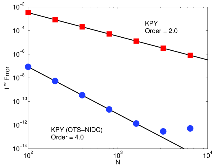
Figure 1: $L^{\infty}$ error as a function of number of grid points for the KPY discretization of the second-order wave equation on with OTS-NIDC (blue circles) and without OTS-NIDC (red squares).

An important property of the KPY scheme is that the error introduced during the first time step affects the global error at all times. More specifically, a $(p+1)$-order accurate first time introduces an $O(\Delta x^{p})$ error into the solution at all future times. Thus, we must ensure that the error introduced by the first time step is at least one order of accuracy higher than desired accuracy for the numerical solution. See Appendix B for a derivation of this condition.

Constructing a fifth-order approximation for the first time step is straightforward using a fifth-order Taylor series expansion in time:

$$u^{1} = u^{0}+\Delta t\frac{\partial u^{0}}{\partial t}+\frac{\Delta t^{2}}{2}\frac{\partial^{2}u^{0}}{\partial t^{2}}+\frac{\Delta t^{3}}{6}\frac{\partial^{3}u^{0}}{\partial t^{3}}+\frac{\Delta t^{4}}{24}\frac{\partial^{4}u^{0}}{\partial t^{4}}$$ (20)

$$= u^{0}+\Delta t\frac{\partial u^{0}}{\partial t}+\frac{\Delta t^{2}}{2}\left(c^{2}\frac{\partial^{2}u^{0}}{\partial x^{2}}+f\right)+\frac{\Delta t^{3}}{6}\left(c^{2}\frac{\partial^{2}}{\partial x^{2}}\left(\frac{\partial u^{0}}{\partial t}\right)+\frac{\partial f}{\partial t}\right)$$

$$+\ \frac{\Delta t^{4}}{24}\left(c^{4}\frac{\partial^{4}u^{0}}{\partial x^{4}}+c^{2}\frac{\partial^{2}f}{\partial x^{2}}+\frac{\partial^{2}f}{\partial t^{2}}\right).$$

Note that special care must be exercised if finite differences are used to compute the derivatives in (20) because higher-order terms may be implicitly included by lower-order terms in the expansion if the initial time step is taken using $\Delta t_{opt}$.

3.3 Diffusion Equation

Solution of the diffusion equation, $u_{t}=Du_{xx}$, using forward Euler time integration with a second-order central difference approximation for the Laplacian provides a familiar example where careful choice of the time step leads to cancellation of the leading order spatial and temporal truncation errors. It is well-known that choosing the time step to be $\Delta t_{opt}=\Delta x^{2}/6D$ boosts the order of accuracy for this simple scheme from $O(\Delta x^{2})$ to $O(\Delta x^{4})$.

When a source term is present, boosting the order of accuracy requires the addition of defect correction terms. These correction terms are straightforward to calculate by examining the discretization error for the scheme

$$u^{n+1}_{j}=u^{n}_{j}+\Delta t\left(D\left[\frac{u^{n}_{j+1}-2u^{n}_{j}+u^{n}_{j-1}}{\Delta x^{2}}\right]+f^{n}_{j}\right),$$ (21)

where $f$ is the source term. Note that even though this scheme is formally first-order in time and second-order in space, the stability constraint $\Delta t\leq\Delta x^{2}/2D$ implies that the scheme is $O(\Delta x^{2})$ accurate overall (i.e. inclusion of the temporal order of accuracy is irrelevant). Using Taylor series expansions and the PDE $u_{t}=Du_{xx}+f$, we see that the true solution satisfies

$$\tilde{u}^{n+1}_{j}=\tilde{u}^{n}_{j} + \Delta t\left(D\frac{\partial^{2}\tilde{u}^{n}}{\partial x^{2}}+f^{n}_{j}\right)$$ (22)

$$+ \frac{(D\Delta t)^{2}}{2}\frac{\partial^{4}\tilde{u}^{n}}{\partial x^{4}}+\frac{\Delta t^{2}}{2}\left(D\frac{\partial^{2}f}{\partial x^{2}}+\frac{\partial f}{\partial t}\right)+O\left(\Delta t^{3}\right)$$

and that the central difference approximation for the Laplacian satisfies

$$\frac{\tilde{u}^{n}_{j+1}-2\tilde{u}^{n}_{j}+\tilde{u}^{n}_{j-1}}{\Delta x^{2}}=\frac{\partial^{2}\tilde{u}^{n}}{\partial x^{2}}+\frac{\Delta x^{2}}{12}\frac{\partial^{4}\tilde{u}^{n}}{\partial x^{4}}+O(\Delta x^{4}).$$ (23)

Therefore, the truncation error for (21) is given by

$$\frac{\partial^{4}\tilde{u}^{n}}{\partial x^{4}}\left[\frac{\Delta x^{2}}{12}-\frac{D\Delta t}{2}\right](D\Delta t)-\frac{\Delta t^{2}}{2}\left(D\frac{\partial^{2}f}{\partial x^{2}}+\frac{\partial f}{\partial t}\right)+O(\Delta t\Delta x^{4})+O(\Delta t^{3}).$$ (24)

From this expression, we easily recover the well-known optimal time step for the diffusion equation, $\Delta t_{opt}=\Delta x^{2}/6D$, and identify the correction term $\Delta t^{2}\left(Df_{xx}+f_{t}\right)/2$.

From (8), we see that using the optimal time step and adding this simple correction term to (21) boosts the accuracy of original scheme from second to fourth order. Note that to achieve fourth order accuracy, the spatial derivatives in the correction term must be calculated using a finite difference approximation that is at least second-order accurate; otherwise, the truncation error will be $O(\Delta t^{2}\Delta x)$ which implies an $O(\Delta t\Delta x)=O(\Delta x^{3})$ global error. The importance of the correction term is illustrated in Figure 2, which compares the accuracy of the OTS forward Euler scheme with and without the correction term. As we can see, OTS forward Euler with correction term is fourth-order accurate while OTS forward Euler without correction term is only second-order accurate.

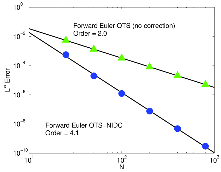
Figure 2: $L^{\infty}$ error as a function of number of grid points for two finite difference schemes that solve the diffusion equation: forward Euler with optimal time step and defect correction term (circles) and forward Euler with optimal time step without defect correction term (triangles).

3.3.1 DuFort-Frankel Scheme

As mentioned earlier, the forward Euler scheme for the diffusion equation is unstable for problems in more than 3 space dimensions. Fortunately, the OTS-NIDC makes it possible to construct a fourth-order accurate DuFort-Frankel scheme.

We begin by writing the DuFort-Frankel scheme in form that is easily generalizable to higher space dimensions:

$$u^{n+1}_{j}=u^{n-1}_{j}+2\Delta t\left(D\left[\frac{u^{n}_{j+1}-2u^{n}_{j}+u^{n}_{j-1}}{\Delta x^{2}}\right]+f^{n}_{j}\right)-2D\frac{\Delta t^{3}}{\Delta x^{2}}\left(\frac{u^{n+1}_{j}-2u^{n}_{j}+u^{n-1}_{j}}{\Delta t^{2}}\right).$$ (25)

Note that the DuFort-Frankel scheme is essentially a leap-frog time integration scheme that is stabilized by the addition of a term proportional to $u_{tt}$ that vanishes in the limit $\Delta t\rightarrow 0$. This scheme is unconditionally stable and has a global error that is formally $O(\Delta t^{2}/\Delta x^{2})+O(\Delta t^{2})+O(\Delta x^{2})+O(\Delta t^{4}/\Delta x^{2})$ [19]. This expression for the formal error is “minimized” when $\Delta t=O(\Delta x^{2})$, which yields an $O(\Delta x^{2})$ global error.

Using Taylor series expansions centered at $(x_{j},t_{n})$, (23) and the PDE to derive the local truncation error for the DuFort-Frankel scheme, we find that

$$\tau = 2D\Delta t\frac{\partial^{4}\tilde{u}}{\partial x^{4}}\left(\frac{\Delta x^{2}}{12}-\frac{D^{2}\Delta t^{2}}{\Delta x^{2}}\right)-2D\frac{\Delta t^{3}}{\Delta x^{2}}\left(D\frac{\partial^{2}f}{\partial x^{2}}+\frac{\partial f}{\partial t}\right)$$ (26)

$$+ O(\Delta t^{3})+O(\Delta t\Delta x^{4})+O\left(\frac{\Delta t^{5}}{\Delta x^{2}}\right).$$

Therefore the optimal time step is $\Delta t_{opt}=\Delta x^{2}/D\sqrt{12}$ and the defect correction term is $2D\Delta t^{3}\left(Df_{xx}+f_{t}\right)/\Delta x^{2}$. As with the forward Euler scheme for the diffusion equation, OTS-NIDC boosts the order of accuracy for the DuFort-Frankel scheme from two to four. Figure 3 shows that OTS-NIDC applied to the DuFort-Frankel scheme achieves the expected boost in accuracy.

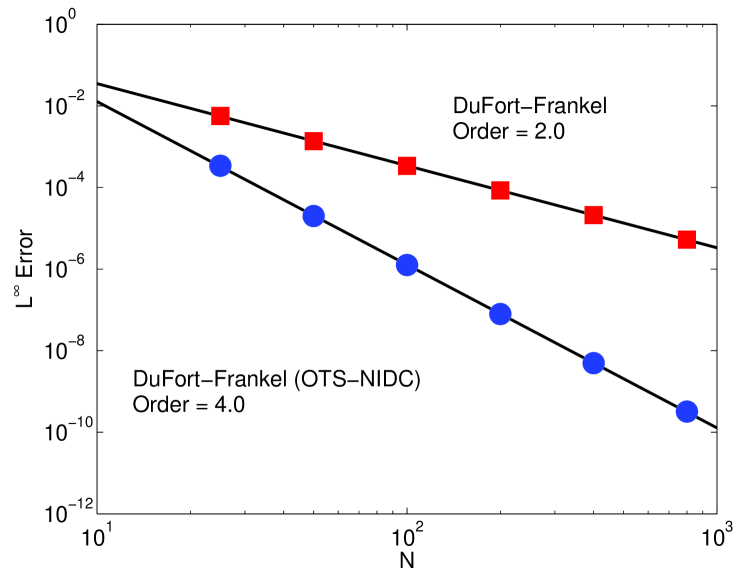
Figure 3: $L^{\infty}$ error in the numerical solution of the 1D diffusion equation as a function of number of grid points for the DuFort-Frankel scheme with (circles) and without (squares) OTS-NIDC.

3.4 Viscous Burgers Equation

We now demonstrate the use of OTS-NIDC in the context of a well-studied semilinear PDE – the viscous Burgers equation [22]:

$$\frac{\partial u}{\partial t}+u\frac{\partial u}{\partial x}=\nu\frac{\partial^{2}u}{\partial x^{2}}$$ (27)

where $\nu$ is the viscosity. For this equation, let us consider the finite difference scheme constructed using a forward Euler time integration scheme and second-order, central difference approximations for the diffusion and nonlinear advection terms:

$$u^{n+1}_{j}=u^{n}_{j}+\Delta t\left(\nu\left[\frac{u^{n}_{j+1}-2u^{n}_{j}+u^{n}_{j-1}}{\Delta x^{2}}\right]-u^{n}_{j}\left[\frac{u^{n}_{j+1}-u^{n}_{j-1}}{2\Delta x}\right]\right).$$ (28)

This scheme is formally first-order in time and second-order in space. Using the stability condition for the advection-diffusion as a heuristic guide, we expect a stability constraint of the form $\Delta t\leq\Delta x^{2}/2\nu$ in the limit $\Delta x\rightarrow 0$ (assuming that the solution $u$ remains bounded). Therefore, the scheme (28) is $O(\Delta x^{2})$ accurate overall.

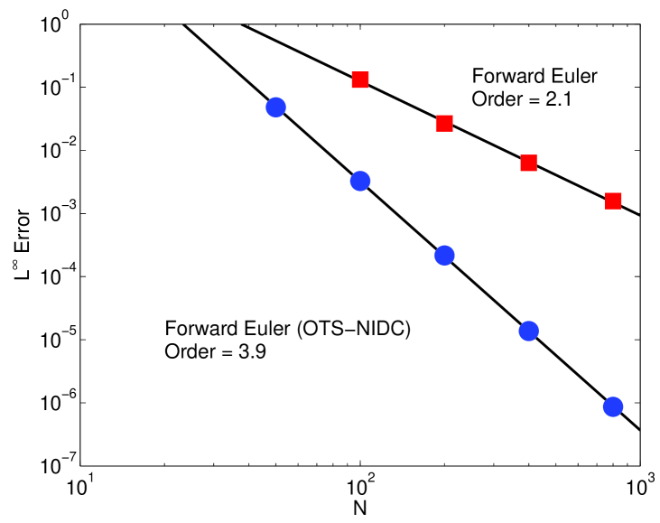
Figure 4: $L^{\infty}$ error as a function of number of grid points for two finite difference schemes that solve the viscous Burgers equation: forward Euler with OTS-NIDC (circles) and forward Euler with suboptimal time step $\Delta t=\Delta x^{2}/4\nu$ and no correction term (squares). The viscous Burgers equation is solved with initial conditions taken to be $u(x,0)=1+\gamma\sqrt{\frac{\nu}{\pi}}\exp\left(-(x-1)^{2}/4\nu\right)/\left[1+\frac{\gamma}{2}\ \mathtt{erfc}\left((x-1)/\sqrt{4\nu}\right)\right]$, where $\ln(1+\gamma)$ is the effective Reynolds number (set equal to 10) and the wave speed is set equal to $1$. The boundary conditions are imposed exactly by using the analytical solution $u(x,t)=1+\gamma\sqrt{\frac{\nu}{\pi T}}\exp\left(-(x-T)^{2}/4\nu T\right)/\left[1+\frac{\gamma}{2}\ \mathtt{erfc}\left((x-T)/\sqrt{4\nu T}\right)\right]$, where $T=t+1$.

To analyze the discretization error for (28), we combine (23) from our analysis of the diffusion equation with the leading-order discretization error for the central difference approximation of $u_{x}$,

$$\frac{\tilde{u}^{n}_{j+1}-\tilde{u}^{n}_{j-1}}{2\Delta x}=\frac{\partial\tilde{u}^{n}}{\partial x}+\frac{\Delta x^{2}}{6}\frac{\partial^{3}\tilde{u}^{n}}{\partial x^{3}}+O(\Delta x^{4}),$$ (29)

to obtain the local truncation error for (28):

$$\left(\nu\frac{\partial^{4}\tilde{u}^{n}}{\partial x^{4}}-2\tilde{u}^{n}_{j}\frac{\partial^{3}\tilde{u}^{n}}{\partial x^{3}}\right)\left[\frac{\Delta x^{2}}{12}-\frac{\nu\Delta t}{2}\right]\Delta t$$ (30)

$$+ \frac{\Delta t^{2}}{2}\left(4\nu\frac{\partial\tilde{u}^{n}}{\partial x}\frac{\partial^{2}\tilde{u}^{n}}{\partial x^{2}}-2\tilde{u}^{n}_{j}\left(\frac{\partial^{2}\tilde{u}^{n}}{\partial x^{2}}\right)^{2}-\left(\tilde{u}^{n}_{j}\right)^{2}\frac{\partial^{2}\tilde{u}^{n}}{\partial x^{2}}\right)$$

$$+ O(\Delta t^{3})+O(\Delta t\Delta x^{4}).$$

Therefore, the optimal time step is $\Delta t_{opt}=\Delta x^{2}/6\nu$ and the defect correction term is

$$-\frac{\Delta t^{2}}{2}\left(4\nu\frac{\partial\tilde{u}^{n}}{\partial x}\frac{\partial^{2}\tilde{u}^{n}}{\partial x^{2}}-2\tilde{u}^{n}_{j}\left(\frac{\partial^{2}\tilde{u}^{n}}{\partial x^{2}}\right)^{2}-\left(\tilde{u}^{n}_{j}\right)^{2}\frac{\partial^{2}\tilde{u}^{n}}{\partial x^{2}}\right)$$ (31)

Note that the optimal time step eliminates errors introduced by both the diffusion term and the nonlinear advection term.

By using the optimal time step and the correction term, the overall error for the finite difference scheme (28) is reduced from $O(\Delta x^{2})$ to $O(\Delta x^{4})$. As for the diffusion equation, we need to use a second-order accurate discretization for the spatial derivatives in the correction term. Figure 4 demonstrates the boost in accuracy obtained by applying OTS-NIDC to the finite difference scheme (28).

The Burgers equation example illustrates an important aspect of OTS-NIDC: the ease with which OTS-NIDC can be used to boost the order of accuracy depends on the choice of the finite difference scheme. Had we chosen an upwind approximation for the gradient term in the Burgers equation, the correction term would have been more complicated and included terms involving higher-order spatial derivatives than those that appear in the original equation. While it should be possible to handle this situation with OTS-NIDC selection, it is clearly less desirable.

3.5 Fourth-Order Parabolic Equation

As a final example in one space dimension, we consider a PDE with high-order spatial derivatives – a fourth-order parabolic equation:

$$\frac{\partial u}{\partial t}=-\kappa\frac{\partial^{4}u}{\partial x^{4}}+f(x,t),$$ (32)

where $\kappa>0$. This example illustrates the importance of the choice of discretization for the spatial derivative in order for OTS-NIDC to be applicable.

From our previous examples, we know that optimal time step selection requires the coefficient on leading-order spatial discretization error to be directly related to the second derivative of the solution $u$ with respect to time:

$$\frac{\partial^{2}u}{\partial t^{2}}=\kappa^{2}\frac{\partial^{8}u}{\partial x^{8}}-\kappa\frac{\partial^{4}f}{\partial x^{4}}+\frac{\partial f}{\partial t}.$$ (33)

Therefore, the leading-order term in the spatial discretization error should involve the eighth-derivative of $u$, which implies that the finite difference approximation to the bilaplacian needs to be at least fourth-order accurate. With this insight, let us consider a finite difference scheme for (32) that uses forward Euler for time integration and a fourth-order central difference approximation for the bilaplacian:

$$u^{n+1}_{j}=u^{n}_{j}+\Delta t\left(-\kappa Bu^{n}+f_{j}^{n}\right),$$ (34)

where the fourth-order discrete bilaplacian is given by

$$Bu^{n}=\frac{-u^{n}_{j+3}+12u^{n}_{j+2}-39u^{n}_{j+1}+56u^{n}_{j}-39u^{n}_{j-1}+12u^{n}_{j-2}-u^{n}_{j-3}}{6\Delta x^{4}}.$$ (35)

This scheme is formally first-order in time and fourth-order in space. Due to the stability constraint $\Delta t\leq 3\Delta x^{4}/40\kappa$, the scheme is $O(\Delta x^{4})$ accurate overall.

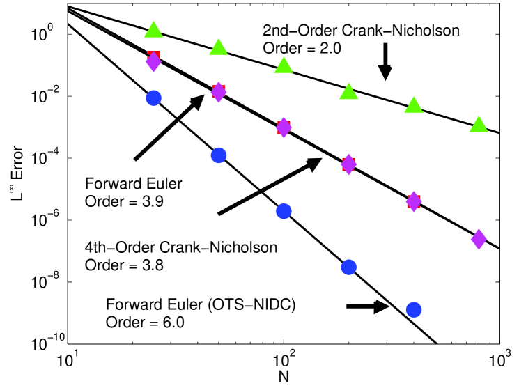
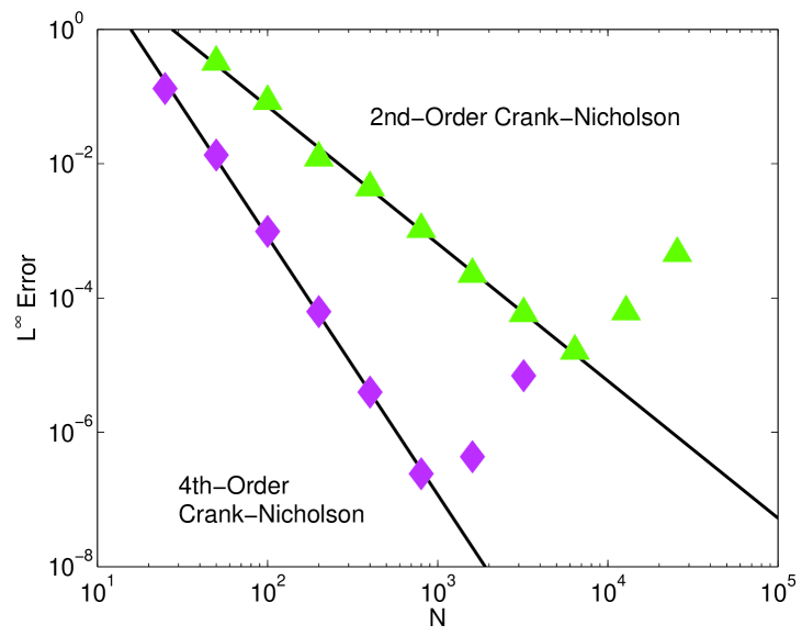
Figure 5: $L^{\infty}$ error as a function of number of grid points for four finite difference schemes that solve the fourth-order parabolic equation (32): forward Euler with OTS-NIDC (circles), forward Euler with suboptimal time step and no correction term (squares), Crank-Nicholson with a fourth-order stencil for the bilaplacian and an $O(\Delta x^{2})$ time step (diamonds), and Crank-Nicholson with a second-order stencil for the bilaplacian (triangles). Both forward Euler schemes use a fourth-order, central finite difference approximation for the bilaplacian. The boundary and ghost cells values are set by taking values from the known analytical solution. Note that the errors for the forward Euler with suboptimal time step and fourth-order Crank-Nicholson schemes lie almost directly on top of each other at the resolution of the figures. The figure on the left highlights the impact (when $N$ is large) of round-off error associated with matrix inversion on the accuracy of the solution for the two Crank-Nicholson schemes.

Proceeding in the usual way, we find that the true solution satisfies

$$\tilde{u}^{n+1}_{j}=\tilde{u}^{n}_{j}+\Delta t\left(-\kappa\frac{\partial^{4}\tilde{u}^{n}}{\partial x^{4}}+f^{n}_{j}\right)+\frac{\Delta t^{2}}{2}\left(\kappa^{2}\frac{\partial^{8}\tilde{u}^{n}}{\partial x^{8}}-\kappa\frac{\partial^{4}f}{\partial x^{4}}+\frac{\partial f}{\partial t}\right)+O\left(\Delta t^{3}\right)$$ (36)

and that the central difference approximation to the bilaplacian satisfies

$$B\tilde{u}^{n}=\frac{\partial^{4}\tilde{u}}{\partial x^{4}}-\frac{7\Delta x^{4}}{240}\frac{\partial^{8}\tilde{u}}{\partial x^{8}}+O(\Delta x^{6}).$$ (37)

Combining these results with the finite difference scheme (34), we find that the local truncation error is given by

$$\frac{\partial^{8}\tilde{u}^{n}}{\partial x^{8}}\left[\frac{7\Delta x^{4}}{240}-\frac{\kappa\Delta t}{2}\right](\kappa\Delta t)+\frac{\Delta t^{2}}{2}\left(\kappa\frac{\partial^{4}f}{\partial x^{4}}-\frac{\partial f}{\partial t}\right)+O(\Delta t^{3})+O(\Delta t\Delta x^{6})$$ (38)

Therefore, the optimal time step is $\Delta t_{opt}=7\Delta x^{4}/120\kappa$ and the correction term is

$$-\frac{\Delta t^{2}}{2}\left(\kappa\frac{\partial^{4}f}{\partial x^{4}}-\frac{\partial f}{\partial t}\right).$$ (39)

Together, these modifications boost the accuracy of the original finite difference scheme from fourth- to sixth-order. As with the previous examples, the spatial derivatives in the correction term should be computed using a finite difference approximation that is at least second-order accurate. The improved accuracy of (34) when the optimal time step and defect correction terms are used is illustrated in Figure 5.

Applying optimal time step selection to high-order PDEs requires the use of high-order discretizations of the spatial derivatives. While the need to derive high-order finite difference stencils may seem like an unnecessary burden, it is important to remember that high-order finite difference schemes for spatial derivatives are almost always necessary to maximize the efficiency of explicit time integration schemes for high-order PDEs. Optimal time step selection merely provides a valuable way to leverage the effort spent deriving high-order finite difference schemes in order to further boost the overall accuracy of the numerical method.

Table 3: Computational cost as a function of the global numerical error $e$ for various finite difference schemes that numerically solve the 1D fourth-order parabolic equation. For all finite difference schemes, the time step is chosen so that the temporal error is subdominant to the spatial error.

Numerical Scheme	$\Delta x$	$\Delta t$	Memory	Compute Time
Forward Euler with	$O\left(e^{1/2}\right)$	$O\left(e^{2}\right)$	$O\left(e^{-1/2}\right)$	$O\left(e^{-5/2}\right)$
2nd-Order Bilaplacian
Forward Euler with	$O\left(e^{1/4}\right)$	$O\left(e\right)$	$O\left(e^{-1/4}\right)$	$O\left(e^{-{5/4}}\right)$
4th-Order Bilaplacian
Forward Euler with	$O\left(e^{1/6}\right)$	$O\left(e^{2/3}\right)$	$O\left(e^{-1/6}\right)$	$O\left(e^{-5/6}\right)$
4th-Order Bilaplacian and OTS-NIDC
Crank-Nicholson with	$O\left(e^{1/2}\right)$	$O\left(e^{1/2}\right)$	$O\left(e^{-1/2}\right)$	$O\left(e^{-1}\right)$
2nd-Order Bilaplacian
Crank-Nicholson with	$O\left(e^{1/4}\right)$	$O\left(e^{1/2}\right)$	$O\left(e^{-1/4}\right)$	$O\left(e^{-3/4}\right)$
4th-Order Bilaplacian

Table 3 shows the computational performance of various finite difference methods for solving equation (33). Observe the dramatic decrease in computational cost as a function of the error by simply replacing a second-order discretization for the bilaplacian operator with a fourth-order discretization. For the forward Euler scheme, using an OTS-NIDC drives the computational cost down even more. The performance plot in Figure 6 shows that the theoretical estimates are in good agreement with timings from computational experiments. Note that the empirical performance for the forward Euler schemes is better than theoretically expected because the computational work per time step is not dominated by the $O(1/\Delta x)$ update calculations until $\Delta x$ gets very small.

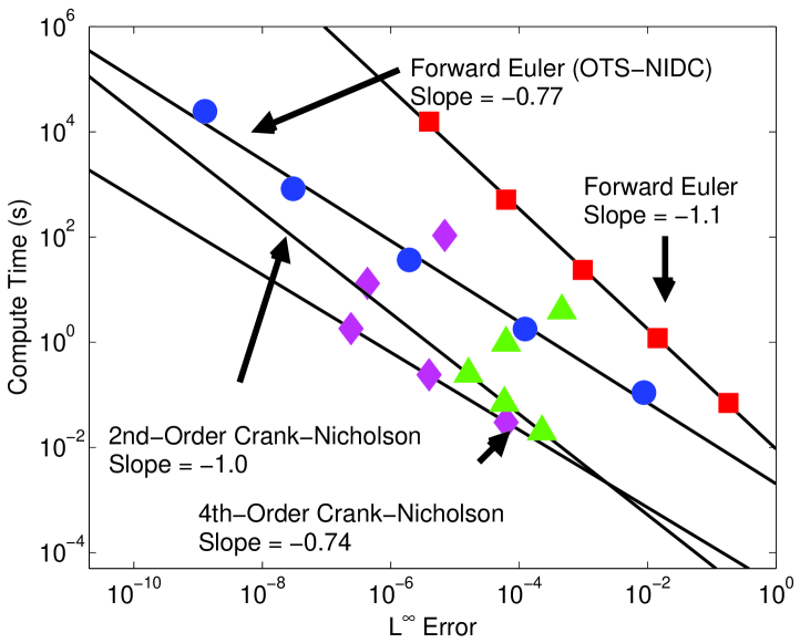
Figure 6: Computation time as a function of $L^{\infty}$ error for four finite difference schemes that solve the fourth-order parabolic equation (32). These results were obtained using MATLAB implementations of the finite difference schemes run on a 2.4 GHz MacBook Pro. Note the impact of round-off error associated with matrix inversion on the accuracy of the solution for the two Crank-Nicholson schemes. See the caption of Figure 5 for descriptions of the four finite difference schemes.

In Figure 6, observe that the 2nd-order Crank-Nicholson scheme actually outperforms the OTS-NIDC scheme over the high (but still practically useful) range of errors even though Table 3 predicts that the OTS-NIDC scheme should do better. The origin of this discrepancy is the constant hidden by the big-$O$ notation. In particular, the factor of $7/120$ in the optimal time step for the forward Euler scheme with a fourth-order approximation of the bilaplacian leads to a relatively large hidden constant for the compute time. However, as Figures 5 and 6 show, there is an important limitation of the 2nd-order Crank-Nicholson scheme even if we ignore the cross-over which will occur at sufficiently small values of the error – round-off error associated with matrix inversion limits the accuracy that is achievable by the scheme. This limitation also exists for the 4th-order Crank-Nicholson scheme.

Comparing the computational cost of the best forward Euler and Crank-Nicholson schemes, we see that the OTS-NIDC forward Euler scheme more efficiently utilizes memory at the cost of requiring more computation time. This tradeoff between memory and computation only exists in one space dimension. In two-dimensions, both schemes require the same amount of compute time; in three or more space dimensions, the forward Euler scheme requires less compute time than the Crank-Nicholson scheme.

4 Application to PDEs in Multiple Space Dimensions

OTS-NIDC can be used to boost the order of accuracy for finite difference schemes in any number of space dimensions. However, several important issues arise for problems in more than one space dimension. These issues are primarily related to the presence of cross-terms in the discretization error, multiple grid spacing parameters, and the domain geometry. In this section, we show how OTS-NIDC selection easily overcomes these issues by using it to construct high-order finite difference schemes for the 2D advection equation and the 2D diffusion equation. It is straightforward to generalize the approach presented in this section to more space dimensions and to construct methods for semilinear PDEs by incorporating ideas discussed in Sections 2 and 3.

4.1 Discretization of Spatial Derivatives

A significant distinction between the error for finite difference schemes in one space dimension and multiple space dimensions is the presence of cross-terms in the discretization error. When formally analyzing the accuracy of a finite difference scheme, it is usually safe to ignore the details of these terms because they can be absorbed within big-$O$ notation. However, precise knowledge of the cross-terms is critical when attempting to use OTS-NIDC. Without this knowledge, it is impossible to ensure cancellation of leading-order errors.

Recall that OTS-NIDC requires the leading-order temporal errors to be directly related to the leading-order spatial errors via the PDE. This requirement can be satisfied in one of two ways:

• by carefully designing the spatial discretization so that the leading-order spatial errors are directly related to the spatial derivative operators in the PDE; or

• by explicitly adding defect correction terms to cancel out any cross-terms in the discretization error that cannot be eliminated by using the PDE.

These two approaches are actually equivalent because the correction terms can be combined with the finite difference stencils in the original scheme and be viewed as part of an alternate spatial discretization scheme.

4.2 Linear Advection Equation

For our first application of OTS-NIDC in multiple space dimensions, we consider the two-dimensional advection equation

$$\frac{\partial u}{\partial t}+\vec{A}\cdot\nabla u=0,$$ (40)

where $\vec{A}=(A_{x},A_{y})$ is the advection velocity. The most interesting and important aspect of this problem is that elimination of the truncation error requires optimal selection of the grid spacing ratio as well as the time step. That is, the more general idea of numerical parameter optimization is needed in order to boost the accuracy of the scheme.

For convenience, let us assume that $A_{x},A_{y}>0$. The simple forward Euler scheme for (40) with first-order upwind discretizations of the advection terms is

$$u^{n+1}_{i,j}=u^{n}_{i,j}-A_{x}\Delta t\left(\frac{u^{n}_{i,j}-u^{n}_{i-1,j}}{\Delta x}\right)-A_{y}\Delta t\left(\frac{u^{n}_{i,j}-u^{n}_{i,j-1}}{\Delta y}\right)$$ (41)

This method is formally first-order in both space and time with a stability constraint of $\Delta t<\left(A_{x}/\Delta x+A_{y}/\Delta y\right)^{-1}$.

To compute the optimal time step and grid spacing ratio, we begin by analyzing the discretization error for (41). As in our analysis of the finite difference scheme for the one-dimensional advection equation, we retain all of the terms in the discretization error. Using Taylor series expansions and the PDE (40), we find that the true solution $\tilde{u}$ satisfies

$$\tilde{u}^{n+1}_{i,j} = \tilde{u}^{n}_{i,j}+\sum_{k=1}^{\infty}\frac{\left(-\Delta t\right)^{k}}{k!}\left(A_{x}\partial_{x}+A_{y}\partial_{y}\right)^{k}\tilde{u}^{n}.$$ (42)

$$\frac{\tilde{u}^{n}_{i,j}-\tilde{u}^{n}_{i-1,j}}{\Delta x} = \frac{\partial\tilde{u}}{\partial x}-\frac{1}{\Delta x}\sum_{k=2}^{\infty}\frac{\left(-\Delta x\right)^{k}}{k!}\frac{\partial^{k}\tilde{u}^{n}}{\partial x^{k}}$$ (43)

$$\frac{\tilde{u}^{n}_{i,j}-\tilde{u}^{n}_{i,j-1}}{\Delta y} = \frac{\partial\tilde{u}}{\partial y}-\frac{1}{\Delta y}\sum_{k=2}^{\infty}\frac{\left(-\Delta y\right)^{k}}{k!}\frac{\partial^{k}\tilde{u}^{n}}{\partial y^{k}}.$$ (44)

Therefore, the local truncation error is given by:

$$\tau^{n}_{i,j} = \frac{A_{x}\Delta t}{2}\frac{\partial^{2}\tilde{u}}{\partial x^{2}}\left(\Delta x-A_{x}\Delta t\right)+\frac{A_{y}\Delta t}{2}\frac{\partial^{2}\tilde{u}}{\partial y^{2}}\left(\Delta y-A_{y}\Delta t\right)-A_{x}A_{y}\Delta t^{2}\frac{\partial^{2}\tilde{u}}{\partial x\partial y}$$ (45)

$$+ \frac{A_{x}\Delta t}{\Delta x}\sum_{k=3}^{\infty}\frac{\left(-\Delta x\right)^{k}}{k!}\frac{\partial^{k}\tilde{u}^{n}}{\partial x^{k}}+\frac{A_{y}\Delta t}{\Delta y}\sum_{k=3}^{\infty}\frac{\left(-\Delta y\right)^{k}}{k!}\frac{\partial^{k}\tilde{u}^{n}}{\partial y^{k}}$$

$$- \sum_{k=3}^{\infty}\frac{\left(-\Delta t\right)^{k}}{k!}\left(A_{x}\partial_{x}+A_{y}\partial_{y}\right)^{k}\tilde{u}^{n}$$

From this expression, we see that choosing the ratio of the grid spacings to be $\Delta x/\Delta y=A_{x}/A_{y}$ and setting the time step to be $\Delta t_{opt}=\Delta x/A_{x}=\Delta y/A_{y}$ eliminates two of the three leading-order terms in the discretization error. The last leading-order term can be eliminated by adding the defect correction term

$$A_{x}A_{y}\Delta t^{2}\frac{\partial^{2}\tilde{u}}{\partial x\partial y}.$$ (46)

These choices enable us to boost the order of accuracy for the finite difference scheme (41) from first- to second-order.

With a careful choice of discretization for the correction term, we can boost the order of accuracy even further. Using the first-order upwind discretization for $\tilde{u}_{xy}$

$$\frac{\left(u_{i,j}-u_{i-1,j}\right)-\left(u_{i,j-1}-u_{i-1,j-1}\right)}{\Delta x\Delta y},$$ (47)

the truncation error (45) becomes

$$\tau^{n}_{i,j} = \frac{A_{x}\Delta t}{2}\frac{\partial^{2}\tilde{u}}{\partial x^{2}}\left(\Delta x-A_{x}\Delta t\right)+\frac{A_{y}\Delta t}{2}\frac{\partial^{2}\tilde{u}}{\partial y^{2}}\left(\Delta y-A_{y}\Delta t\right)$$ (48)

$$+ \frac{A_{x}\Delta t}{\Delta x\Delta y}(\Delta y-A_{y}\Delta t)\sum_{k=3}^{\infty}\frac{\left(-\Delta x\right)^{k}}{k!}\frac{\partial^{k}\tilde{u}^{n}}{\partial x^{k}}$$

$$+ \frac{A_{y}\Delta t}{\Delta x\Delta y}(\Delta x-A_{x}\Delta t)\sum_{k=3}^{\infty}\frac{\left(-\Delta y\right)^{k}}{k!}\frac{\partial^{k}\tilde{u}^{n}}{\partial y^{k}}$$

$$+ \frac{A_{x}A_{y}\Delta t^{2}}{\Delta x\Delta y}\sum_{k=3}^{\infty}\sum_{l=0}^{k}(-1)^{k}{k\choose l}\frac{\Delta x^{l}\Delta y^{k-l}}{k!}\frac{\partial^{k}\tilde{u}^{n}}{\partial x^{l}\partial y^{k-l}}$$

$$- \sum_{k=3}^{\infty}\frac{\left(-\Delta t\right)^{k}}{k!}\left(A_{x}\partial_{x}+A_{y}\partial_{y}\right)^{k}\tilde{u}^{n},$$

which vanishes when the optimal time step and grid spacing ratio are used. In other words, when the defect correction (47) is used in conjunction with the optimal time step and grid spacing ratio, we obtain a finite difference scheme that introduces no truncation error at each time step. Figure 7 demonstrates the amazing accuracy of this scheme over the first-order forward Euler scheme (41) without any modifications. Notice how the sharp corners of the initial conditions are perfectly preserved when the optimal time step, optimal grid spacing ratio, and correction term are used. In contrast, the sharp corners are completely smoothed out in the solution computed using the standard first-order upwind scheme.

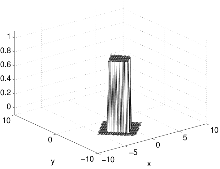
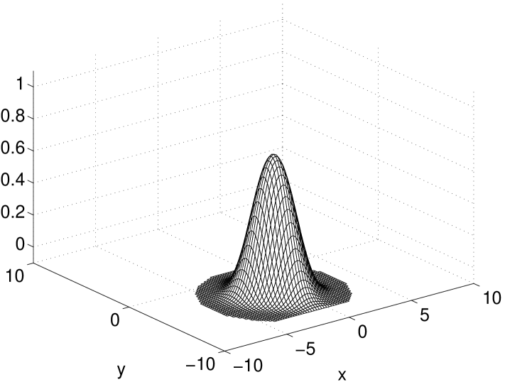
Figure 7: Comparison of numerical solutions for the 2D advection equation (40) using forward Euler time stepping with OTS-NIDC (left) and forward Euler time stepping with suboptimal time step (right). The latter scheme uses a time step $\Delta t=\Delta x/2(|A_{x}|+|A_{y}|)$. Both figures show the numerical solution at $t=3$ computed on the domain $-10<x,y<10$ using 100 grid points in each direction. The advection velocity $(A_{x},A_{y})$ is set to $(-1,-2)$. The initial conditions are taken to be a 2D square function centered at the origin: $u(x,y,0)=1$ if $|x|+|y|\leq 2$ and $u(x,y,0)=0$ if $|x|+|y|>2$. For the time interval considered, $u$ is identically zero on the boundary.

It is interesting to push the analysis of the optimal finite difference scheme a little further and examine the complete finite difference scheme (including defect correction term):

$$u^{n+1}_{i,j}=u^{n}_{i,j} - A_{x}\Delta t\left(\frac{u^{n}_{i,j}-u^{n}_{i-1,j}}{\Delta x}\right)-A_{y}\Delta t\left(\frac{u^{n}_{i,j}-u^{n}_{i,j-1}}{\Delta y}\right)$$ (49)

$$+ A_{x}A_{y}\Delta t^{2}\left(\frac{u_{i,j}-u_{i-1,j}-u_{i,j-1}+u_{i-1,j-1}}{\Delta x\Delta y}\right).$$

Using the relationship between the optimal time step and the grid spacing ratio, this scheme can be rewritten as

$$u^{n+1}_{i,j}=u^{n}_{i,j} - \frac{A_{x}\Delta t}{2}\left(\frac{u^{n}_{i,j}-u^{n}_{i-1,j}}{\Delta x}+\frac{u^{n}_{i,j-1}-u^{n}_{i-1,j-1}}{\Delta x}\right)$$ (50)

$$- \frac{A_{y}\Delta t}{2}\left(\frac{u^{n}_{i,j}-u^{n}_{i,j-1}}{\Delta y}+\frac{u^{n}_{i-1,j}-u^{n}_{i-1,j-1}}{\Delta y}\right),$$

which is essentially a forward Euler time integration scheme with first-order upwind discretizations of the spatial derivatives that are computed using all four upwind neighbors. This formulation of (49) suggests that the highest accuracy finite difference scheme for the 2D linear advection equation arises by using a fully upwind discretization of the advection terms with the optimal time step and optimal ratio of grid spacings.

In higher space dimensions, it becomes tedious to carry out the analysis to derive the infinite order accurate finite difference scheme for the advection equation because many high-order correction terms must be retained. However, it is straightforward to generalize (50) to $d$ space dimensions by using first-order discretizations for the spatial derivatives that are averages over the $2^{d-1}$ upwind discretizations in each coordinate direction. As with the two-dimensional problem, the optimal grid spacings satisfy $\Delta x_{k}/A_{x_{k}}=\Delta t_{opt}$ for $1\leq k\leq d$.

Like the unit CFL condition for the one-dimensional advection equation, the analogue of (50) in any number of space dimensions could also have been derived by examining how characteristic lines of the $d$-dimensional advection equation pass through grid points. For the two-dimensional problem, this perspective becomes apparent when we fully simplify (50) using the optimal time step and grid spacing ratio to obtain $u^{n+1}_{i,j}=u^{n}_{i-1,j-1}$.

4.3 Diffusion Equation

As for PDEs in one space dimension, achieving infinite order accuracy through OTS-NIDC is unique to the advection equation. To illustrate the typical accuracy boost gained by using OTS-NIDC, we apply it to the 2D diffusion equation. This example underscores the need to carefully choose the discretization for the spatial derivatives for problems in more than one space dimension and demonstrates the ease with which OTS-NIDC selection can be applied to problems on irregular domains.

In two space dimensions, the diffusion equation may be written as

$$\frac{\partial u}{\partial t}=D\nabla^{2}u+f(x,y,t).$$ (51)

The most common finite difference schemes for (51) employ a five-point, second-order central difference stencil for the Laplacian:

$$L^{5pt}u=\frac{u_{i,j+1}+u_{i,j-1}+u_{i+1,j}+u_{i-1,j}-4u_{i,j}}{\Delta x^{2}},$$ (52)

which assumes that the grid spacing in the $x$ and $y$ directions are equal. The forward Euler scheme using the five-point stencil is given by

$$u^{n+1}_{j}=u^{n}_{j}+\Delta t\left(D\left[\frac{u^{n}_{i,j+1}+u^{n}_{i,j-1}+u^{n}_{i+1,j}+u^{n}_{i-1,j}-4u^{n}_{i,j}}{\Delta x^{2}}\right]+f_{i,j}^{n}\right).$$ (53)

This scheme is formally first-order in time and second-order in space. The stability constraint $\Delta t\leq\Delta x^{2}/4D$ implies that this scheme is $O(\Delta x^{2})$ accurate overall.

While it is certainly possible to directly apply OTS-NIDC to (53), we would be forced to use additional defect correction terms to deal with the fact that the leading-order error for (52), $\Delta x^{2}\left(\tilde{u}_{xxxx}+\tilde{u}_{yyyy}\right)/12$, cannot be directly related to the spatial derivative operator in the diffusion equation. The analysis is more straightforward if we construct our finite difference scheme using the nine-point stencil for the Laplacian [17, 25], which possesses a leading-order error directly related to the spatial derivative operator in the PDE (51):

$$L^{9pt}u=\frac{1}{6\Delta x^{2}}\left(\begin{array}[]{l}\ \ \ u_{i+1,j+1}+u_{i+1,j-1}+u_{i-1,j+1}+u_{i-1,j-1}\\ +\ 4u_{i+1,j}+4u_{i-1,j}+4u_{i,j+1}+4u_{i,j-1}-20u_{i,j}\end{array}\right).$$ (54)

Observe that the nine-point stencil is simply the standard five-point stencil plus $\Delta x^{2}/6$ times a second-order, central difference approximation to $u_{xxyy}$. Therefore, we can obtain the leading-order error in the nine-point stencil by combining the leading-order error for the five-point stencil with the extra contribution of $\Delta x^{2}\tilde{u}_{xxyy}/6$

$$L^{9pt}\tilde{u} = \nabla^{2}\tilde{u}+\frac{\Delta x^{2}}{12}\left(\tilde{u}_{xxxx}+2\tilde{u}_{xxyy}+\tilde{u}_{yyyy}\right)+O(\Delta x^{4})$$ (55)

$$= \nabla^{2}\tilde{u}+\frac{\Delta x^{2}}{12}\nabla^{4}\tilde{u}+O(\Delta x^{4}).$$

Like (53), the forward Euler scheme that uses the nine-point discretization of the Laplacian

$$u^{n+1}_{i,j}=u^{n}_{i,j}+\Delta t\left(DL^{9pt}u+f_{i,j}^{n}\right)$$ (56)

is $O(\Delta x^{2})$ accurate overall because it has a stability constraint $\Delta t\leq 3\Delta x^{2}/8D=O(\Delta x^{2})$. It is interesting to note that use of a nine-point stencil for the Laplacian naturally arises when directly applying OTS-NIDC to the five-point scheme if the defect correction term is interpreted as a modification to the original spatial discretization.

To apply OTS-NIDC to (56), we proceed in the usual way by first analyzing the leading-order terms of the local truncation error for the finite difference scheme:

$$\nabla^{4}\tilde{u}\left[\frac{\Delta x^{2}}{12}-\frac{D\Delta t}{2}\right](D\Delta t)-\frac{\Delta t^{2}}{2}\left(D\nabla^{2}f+\frac{\partial f}{\partial t}\right)+O(\Delta t^{3})+O(\Delta t\Delta x^{4}).$$ (57)

Therefore, the optimal time step is given by $\Delta t_{opt}=\Delta x^{2}/6D$ and the defect correction term is $\Delta t^{2}\left(D\nabla^{2}f+f_{t}\right)$. This choice of time step and correction term yields a scheme that is fourth-order accurate. It is interesting to note that the optimal time step for the forward Euler scheme for the diffusion equation is independent of the number of spatial dimensions.

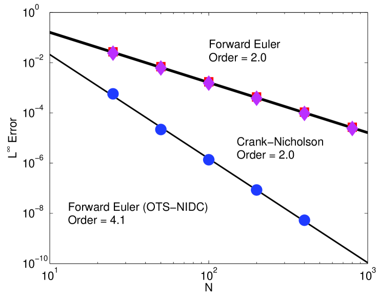
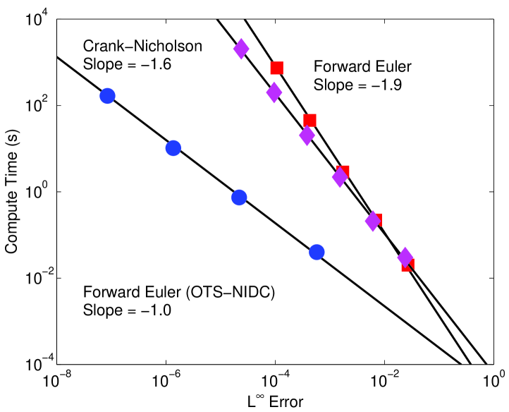
Figure 8: $L^{\infty}$ error as a function of number of grid points in each coordinate direction (left) and computation time as a function of $L^{\infty}$ error (right) for three finite difference schemes that solve the 2D diffusion equation: forward Euler with OTS-NIDC (circles), forward Euler with suboptimal time step (squares), and Crank-Nicholson (diamonds). The forward Euler schemes use a nine-point discretization of the Laplacian; the Crank-Nicholson scheme uses the standard five-point discretization of the Laplacian. Note that the errors for the forward Euler with suboptimal time step and Crank-Nicholson schemes lie almost directly on top of each other at the resolution of the figures. These results were obtained using MATLAB implementations of the finite difference schemes run on a 2.4 GHz MacBook Pro.

The improvement in the accuracy of the forward Euler scheme with OTS-NIDC is shown in Figure 8. Figure 8 also shows that the scaling of the computational time with the error is in good agreement with the theoretical estimates given in Table 2. As with the other examples, the forward Euler scheme with OTS-NIDC is much more computationally efficient than the two other schemes.

4.3.1 Irregular Domains

All of the examples we have considered so far share an important feature: they are all defined on simple, rectangular domains. Any of several methods could have been used to obtain solutions with similar or even higher accuracy. For example, a fourth-order accurate solution to the diffusion equation (in any number of space dimensions) could be obtained by using a pseudospectral spatial discretization [26, 27] of the Laplacian and a fourth-order time integration scheme (e.g. Runge-Kutta). When the domain is irregularly shaped, high-order methods are harder to design and implement. In this section, we extend the OTS-NIDC finite difference scheme for the 2D diffusion equation on regular domains to irregular domains. Other researchers have developed fourth-order accurate methods for the diffusion equation on irregular domains [3, 4]. However, these earlier methods require a wider ghost cell region [3], use implicit time integration [3, 4], or involve a more complex calculation for the boundary conditions [4]. As we shall see, it is possible to achieve fourth-order accuracy for the diffusion equation on irregular domains using only forward Euler integration and a compact, second-order stencil for the Laplacian.

Figure 9: Illustrations of edge (left) and corner (right) ghost cells. The edge ghost cell, $u_{E}$, is filled by using cubic extrapolation of the value on the boundary, $u_{B}$, and values at three interior grid points. The corner ghost cell, $u_{C}$, is filled by using a fourth-order accurate Taylor series expansion centered at $u_{0,0}$, which uses the values of $u$ at the specified interior grid points and neighboring edge ghost cells to approximate the partial derivatives in the expansion.

To avoid the need for special stencils at grid points near the irregular boundary, we adopt the ‘ghost cell’ approach for imposing boundary conditions [3, 4, 15, 16]. The main challenge in using the ghost cell method is ensuring ghost cells are filled using a sufficiently high-order extrapolation scheme. Figure 9 shows examples of ghost cells that lie in the vicinity of an irregular boundary. Notice that there are two types of ghost cells: edge and corner. Edge and corner ghost cells are distinguished by the relative position of the nearest interior grid point. An edge ghost cell is linked to its nearest interior neighbor by an edge of the computational grid whereas a corner ghost cell and its nearest interior neighbor lie on the opposite corners of a grid cell.

To set the value of $u$ in each edge ghost cell, we use 1D cubic (i.e. fourth-order accurate) extrapolation of the values of $u$ across the interface. A cubic Lagrange interpolant is constructed for each edge ghost cell using a point on the domain boundary and three interior grid points that lie along the line parallel to the edge connecting the ghost cell to its nearest interior neighbor (see Figure 9). Because the quality of the interpolant deteriorates if the boundary point $u_{B}$ is too close to any of the interior grid points used to construct the Lagrange extrapolant, we follow [3] and choose the interior grid points so that the nearest interior grid point is sufficiently far from the boundary point. Without this procedure, the errors introduced in the values of the ghost cells lead to instability of the numerical method. Gibou et al. suggest shifting the interpolation points by one grid point when the distance between the boundary point and the nearest interior grid point is less than $\Delta x^{2}$ [3]. For the numerical scheme presented in this article, this threshold was too low. Better stability was obtained if an $O(\Delta x)$ threshold was used.

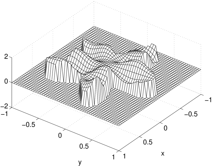
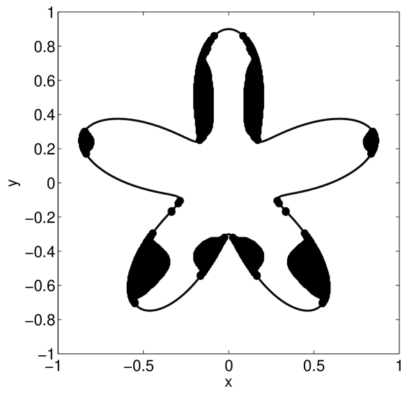
Figure 10: Numerical solutions (left) and dominant error (right) for the 2D diffusion equation on a starfish-shaped domain. The solution is computed using forward Euler time stepping with OTS-NIDC. In the error plot, the dark regions represent points where the error in the solution is larger than $25$% of the $L^{\infty}$ error of the solution.

To set the value of $u$ in a corner ghost cell, we use a fourth-order accurate Taylor series expansion of $u$ centered at the nearest interior neighbor. The partial derivatives in the Taylor series expansion are approximated using finite differences constructed from the values of $u$ at interior grid points and the neighboring edge ghost cells (see Figure 9). For the corner ghost cell shown in Figure 9, the extrapolation stencil is given by

$$u_{C} = -4u_{0,0}-u_{-1,-1}+2u_{1,0}+2u_{0,1}-u_{1,-1}-u_{-1,1}+2u_{0,-1}+2u_{-1,0}$$ (58)

where $u_{C}$ and $u_{i,j}$ are indicated in the figure. The stencils for corner ghost cells that are in other positions relative to the interior of the domain are obtained by rotations of Figure 9 and remapping of the indices in the above stencil.

Using these methods for filling edge and corner ghost cells, it is straightforward to compute high-order accurate solutions of the 2D diffusion equation on irregular domains. We simply use the OTS-NIDC forward Euler scheme designed for regular domains for grid points in the interior of the domain after filling the ghost cells with high-order accurate values. Figure 10 shows an example of a solution computed on a starfish shaped domain. It also shows that the error in the solution is concentrated near the boundaries of the irregular domain. The improved accuracy of the OTS-NIDC solution compared to a simple forward Euler scheme with a suboptimal time step is illustrated in Figure 11.

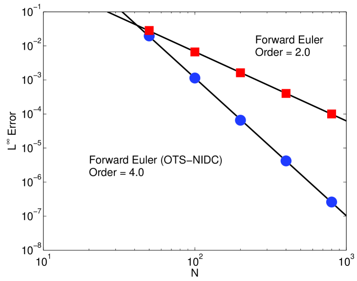
Figure 11: $L^{\infty}$ error as a function of number of grid points in each coordinate direction for two finite difference schemes that solve the 2D diffusion equation on an irregular domain: forward Euler with OTS-NIDC (circles) and forward Euler with suboptimal time step (squares).

4.3.2 Diffusion Equation in Higher Dimensions

Using OTS-NIDC to boost the accuracy of finite difference schemes for the diffusion equation in higher space dimensions is straightforward. As for the 2D problem, the key step is identification of a finite difference stencil for the Laplacian that has an isotropic discretization error. For 3D problems, a catalog of several such stencils is available in [25]. For higher dimensional problems, one simple approach for deriving an isotropic finite difference stencil for the Laplacian would be to start with the generalization of the standard five point stencil for the 2D Laplacian and add finite difference approximations for the missing cross terms that are required to make the leading-order error isotropic (i.e. proportional to the bilaplacian of the solution). Because the missing terms are all of the form

$$\frac{\Delta x^{2}}{6}\left(\frac{\partial^{4}u}{\partial x_{i}^{2}\partial x_{j}^{2}}\right),$$ (59)

this approach is relatively easy to use. To derive finite difference approximations with more general or complex properties, symbolic algebra software can be helpful [25, 28].

Once an acceptable finite difference approximation for the Laplacian has been chosen, the usual OTS analysis yields an optimal time step of $\Delta t_{opt}=\Delta x^{2}/6D$ for forward Euler time integration and a boost of the order of accuracy from two to four. Above three dimensions, the optimal time step is no longer stable, and the forward Euler scheme should be replaced with the DuFort-Frankel scheme (see Section 3.3.1).

Problems on irregular domains can be handled using the ghost cell approach. While the derivation of high accuracy stencils for ghost cells becomes more tedious, the general approach is the same as for the 2D problem. The ghost cells can first be grouped into separate classes based on the number of grid cell edges that must be traversed to reach the nearest interior neighbor. The values in the ghost cells can then be set in order starting with those directly connected to their nearest interior neighbor and ending with those whose nearest interior neighbor is on the opposite corner of a grid cell. Here, too, symbolic algebra programs can be helpful when deriving methods for extrapolating interior and boundary values to ghost cells.

5 Summary

In this article, we have presented OTS-NIDC, a simple approach for constructing high-order finite difference methods for time dependent PDEs without requiring the use of high-order stencils or high-order time integration schemes. The major idea underlying OTS-NIDC is that spatial and temporal discretization errors can be simultaneously eliminated by (1) using the PDE to relate terms in the discretization error, (2) optimally selecting numerical parameters, and (3) adding a few defect correction terms in a non-iterative manner. The boost in the order of accuracy achieved by using OTS-NIDC is well worth the extra effort required to derive the optimal time step and defect correction terms.

Through many examples, we have demonstrated the utility of OTS-NIDC to several types of finite difference schemes for a wide range of problems. We showed how OTS-NIDC can be used to very easily obtain high-order accurate solutions to many linear and semilinear PDEs in any number of space dimensions on both regular and irregular domains. The examples illustrate the high-order of accuracy that can be achieved using only low-order discretizations for spatial derivatives and simple forward Euler time integration. They also demonstrate the applicability of OTS-NIDC to more exotic finite difference schemes, such as the Kreiss-Petersson-Yström discretization of the second-order wave equation and the DuFort-Frankel scheme for the diffusion equation.

Optimal time step selection is an example of the more general technique of optimally selecting numerical parameters to boost the accuracy of numerical methods. Little research appears to have been done in this area, but as OTS-NIDC selection demonstrates, optimal selection of numerical parameters can significantly impact the accuracy of numerical methods. To realize the full potential of existing and novel numerical schemes, both optimal time step selection and optimal numerical parameter selection deserve further investigation and attention.

Appendix A Formal vs. Practical Accuracy

For time dependent PDEs, evaluating the order of accuracy for a numerical method is subtle because there are formally two separate orders of accuracy to consider: temporal and spatial. While it is theoretically interesting and important to understand how the error depends on both the grid spacing $\Delta x$ and the time step $\Delta t$, in practice, the accuracy of a numerical scheme is always controlled by only one of the two numerical parameters.

Even though spatial and temporal orders of accuracy for a numerical method are formally separate, one will always dominate for a given choice of $\Delta x$ and $\Delta t$. For example, when solving the diffusion equation using the backward Euler method for time integration with a second-order central difference stencil for the Laplacian, formal analysis shows that the global error is $O(\Delta x^{2})+O(\Delta t)$. Since there are no stability constraints on the numerical parameters, the time step and grid spacing are free to vary independently. In this situation, the practical error for the method depends on the relative sizes of the time step and grid spacing. When $\Delta t\gg\Delta x^{2}$, the practical error is $O(\Delta t)$ which means that the error in the numerical solution is primarily controlled by the time step. Similarly, when $\Delta t\ll\Delta x^{2}$, the practical error is $O(\Delta x^{2})$ so that the error is controlled by the grid spacing. Finally, when $\Delta t=O(\Delta x^{2})$, the practical error is $O(\Delta t)=O(\Delta x^{2})$. In all cases, the practical error is primarily controlled by one of the two numerical parameters, and varying the subdominant parameter while holding the dominant parameter fixed does not significantly affect the error.

When there are constraints on the numerical parameters, there is less freedom in choosing the controlling parameter. For instance, if we solve the diffusion equation using a forward Euler time integration scheme with a second-order central difference stencil for the Laplacian, stability considerations require that we choose $\Delta t=O(\Delta x^{2})$. Combining this stability constraint with the formal error for the scheme shows that the practical error is $O(\Delta x^{2})+O(\Delta t)=O(\Delta x^{2})$. Therefore, the accuracy of the method is completely controlled by the grid spacing; the temporal error can never dominate the spatial error.

Appendix B Importance of High-Accuracy for First Time Step for the KPY Scheme

The need for higher-order accuracy when taking the first time step of the KPY scheme for the second-order wave equation can be understood by solving the difference equation

$$\hat{e}^{n+1}-2\hat{e}^{n}+\hat{e}^{n-1}=\Delta t^{2}\lambda\hat{e}^{n},$$ (60)

for the normal modes of the error, where $\hat{e}$ is the coefficient of an arbitrary normal mode of the spatial operator for the error $e\equiv u-\tilde{u}$. Using standard methods for solving linear difference equations [29] yields the solution

$$\hat{e}^{n}=\hat{e}^{1}\frac{\kappa_{+}^{n}-\kappa_{-}^{n}}{\kappa_{+}-\kappa_{-}}+\hat{e}^{0}\kappa_{+}\kappa_{-}\frac{\kappa_{+}^{n-1}-\kappa_{-}^{n-1}}{\kappa_{+}-\kappa_{-}},$$ (61)

where $\kappa_{\pm}$ are the roots of the characteristic equation for (60) [21]

$$\kappa_{\pm}=1+\frac{1}{2}\lambda\Delta t^{2}\pm\Delta t\sqrt{\lambda+\frac{\lambda^{2}\Delta t^{2}}{4}}.$$ (62)

Notice that the denominator of both terms in (61) is $O(\Delta t)$, which implies that the error in the initial conditions is degraded by one temporal order of accuracy by the KPY scheme. Therefore, KPY without OTS-NIDC requires the first time step must be at least third-order accurate; KPY with OTS-NIDC requires the first time step must be at least fifth-order accurate.

References

- [1] W. F. Spotz and G. F. Carey. Extension of high-order compact schemes to time-dependent problems. Numer. Meth. Part. D. E., 17:657–672, 2001.
- [2] A. Brüger, B. Gustafsson, P. Lötstedt, and J. Nilsson. High order accurate solution of the incompressible Navier-Stokes equations. J. Comput. Phys., 203:49–71, 2005.
- [3] F. Gibou and R. Fedkiw. A fourth order accurate discretization for the Laplace and heat equations on arbitrary domains, with applications to the Stefan problem. J. Comput. Phys., 202:577–601, 2005.
- [4] K. Ito, Z. Li, and Y. Kyei. Higher-order, Cartesian Grid Based Finite Difference Schemes for Elliptic Equations on Irregular Domains. SIAM J. Sci. Comput., 27:346–367, 2005.
- [5] R. K. Shukla and X. Zhong. Derivation of high-order compact finite difference schemes for non-uniform grid using polynomial interpolation. J. Comput. Phys., 204:404–429, 2005.
- [6] E. A. Heidenreich, J. F. Rodríguez, F. J. Gaspar, and M. Doblaré. Fourth-order compact schemes with adaptive time step for monodomain reaction-diffusion equations. J. Comput. Appl. Math., 216:39–55, 2007.
- [7] R. K. Shukla, M. Tatineni, and X. Zhong. Very high-order compact finite difference schemes on non-uniform grids for incompressible Navier-Stokes equations. J. Comput. Phys., 224:1064–1094, 2007.
- [8] R. J. LeVeque. Finite Volume Methods for Hyperbolic Problems. Cambridge University Press, Cambridge, UK, 2002.
- [9] F. Zhao. Weighting Factors for Single-Step Trapezoidal Method. J. Heat Transf.-Trans. ASME, 128:409–412, 2006.
- [10] V. Pereyra. Iterated Deferred Corrections for Nonlinear Boundary Value Problems. Numer. Math., 11:111–125, 1968.
- [11] H. J. Stetter. The Defect Correction Principle and Discretization Methods. Numer. Math., 29:425–443, 1978.
- [12] B. Gustafsson and L. Hemmingsson-Frn̈dén. Deferred correction in space and time. J. Sci. Comput., 17:541–550, 2002.
- [13] W. Kress and B. Gustafsson. Deferred correction methods for initial boundary value problems. J. Sci. Comput., 17:241–251, 2002.
- [14] W. Kress. Error estimates for deferred correction methods in time. Apll. Numer. Math, 57:335–353, 2006.
- [15] R. Fedkiw, T. Aslam, B. Merriman, and S. Osher. A Non-Oscillatory Eulerian Approach to Interfaces in Multimaterial Flows (The Ghost Fluid Method). J. Comput. Phys., 152:457–492, 1999.
- [16] S. Osher and R. Fedkiw. Level Set Methods and Dynamic Implicit Surfaces. Springer, New York, NY, 2003.
- [17] A. Iserles. A First Course in the Numerical Analysis of Differential Equations. Cambridge University Press, Cambridge, UK, 1996.
- [18] L.F. Shampine. Error Estimation and Control for ODEs. J. Sci. Comput., 25:3–16, 2005.
- [19] B. Gustafsson, H.-O. Kreiss, and J. Oliger. Time Dependent Problems and Difference Methods. John Wiley & Sons, Inc., New York, NY, 1995.
- [20] R. J. LeVeque. Numerical Methods for Conservation Laws. Birkhäuser Verlag, Berlin, 1992.
- [21] H.-O. Kreiss, N. A. Petersson, and J. Yström. Difference Approximations for the Second Order Wave Equation. SIAM. J. Numer. Anal, 40:1940–1967, 2002.
- [22] G. B. Whitham. Linear and Nonlinear Waves. John Wiley & Sons, Inc., New York, NY, 1999.
- [23] T. Chan. Stability Analysis of Finite Difference Schemes for the Avection-Diffusion Equation. SIAM J. Numer. Anal., 21:272–284, 1984.
- [24] J. B. Greer, A. L. Bertozzi, and G. Sapiro. Fourth order partial differential equations on general geometries. J. Comput. Phys., 216:216–246, 2006.
- [25] M. Patra and M. Karttunen. Stencils with Isotropic Discretization Error for Differential Operators. Numer. Meth. for Part. Diff. Eq., 22:936–953, 2005.
- [26] L. N. Trefethen. Spectral Methods in MATLAB. SIAM, Philadelphia, PA, 2000.
- [27] J. P. Boyd. Chebyshev and Fourier Spectral Methods. Dover Publications, Inc., Mineola, NY, 2nd edition, 2001.
- [28] M. M. Gupta and J. Kouatchou. Symbolic Derivation of Finite Difference Approximations for the Three-Dimensional Poisson Equation. Numer. Meth. for Part. Diff. Eq., 14:593–606, 1998.
- [29] G. F. Carrier and C. E. Pearson. Ordinary Differential Equations. Society for Industrial and Applied Mathematics, Philadelphia, 1991.