Magnetic order, Bose-Einstein condensation, and superfluidity
in a bosonic $t$-$J$ model of CP¹ spinons and doped Higgs holons

Abstract

We study the three-dimensional U(1) lattice gauge theory of a CP¹ spinon (Schwinger boson) field and a Higgs field. It is a bosonic $t$-$J$ model in slave-particle representation, describing the antiferromagnetic (AF) Heisenberg spin model with doped bosonic holes expressed by the Higgs field. The spinon coupling term of the action favors AF long-range order, whereas the holon hopping term in the ferromagnetic channel favors Bose-Einstein condensation (BEC) of holons. We investigate the phase structure by means of Monte-Carlo simulations and study an interplay of AF order and BEC of holes. We consider the two variations of the model; (i) the three-dimensional model at finite temperatures, and (ii) the two-dimensional model at vanishing temperature. In the model (i) we find that the AF order and BEC coexist at low temperatures and certain hole concentrations. In the model (ii), by varying the hole concentration and the stiffness of AF spin coupling, we find a phase diagram similar to the model (i). Implications of the results to systems of cold atoms and the fermionic $t$-$J$ model of strongly-correlated electrons are discussed.

I Introduction

In recent years, cold atoms have attracted interest of many condensed-matter physicists. Systems of cold atoms have exhibited (and shall exhibit) various interesting properties like Bose-Einstein condensation (BEC), superfluidity (SF) caused by the BEC, magnetic ordering, etc. Both for condensed-matter experimentalists and theorists cold atoms offer an ideal testing ground to develop and check their ideas because one can precisely control parameters characterizing these systems like dimensionality of the system, strength of interaction among atoms, concentration of atoms, etc. An example of these ideas is a possible interplay of magnetic ordering and BEC (or equivalently SF), although coexistence of these two orders seems not to have been reported experimentally so far.

A standard model of cold bosonic atoms with repulsive interactions may be the bosonic Hubbard model in which electrons are replaced by bosonic atoms. For definiteness, one may consider hard-core bosons to describe these bosons. Then, from such a bosonic Hubbard model one may derive the bosonic $t$-$J$ model as its effective model for the case of strong on-site repulsion and small hole concentrations. This derivation is achieved just by following the steps developed in the theory of high-$T_{\rm c}$ superconductivity to derive the fermionic $t$-$J$ model from the standard Hubbard model by tracing out the double-occupancy states.

Therefore, to study the interplay of magnetic ordering and BEC of bosonic atoms, it is natural to start from the bosonic $t$-$J$ model. In fact, very recently, Boninsegni and Prokof’evbtj studied this phenomenon by using the bosonic $t$-$J$ model where each bosonic electron is considered as a hard-core boson. They applied this model to study bosonic cold atomscold_boson ; cold . Because the model is purely bosonic, one can employ numerical analysis. By quantum Monte Carlo(MC) simulations, they studied the low-temperature ($T$) phase diagram of the two-dimensional (2D) model for the case of anisotropic spin coupling $J_{x,y}=\alpha J_{z},\alpha<1,$ and found the coexistence region of AF order and BEC as a result of the phase separation of hole-free and hole-rich phases.

The bosonic $t$-$J$ model has another important reason to study, i.e., it resembles to the fermionic $t$-$J$ model of the high-temperature superconductors. There the interplay of magnetism and superconductivity(SC) is of interest as one of the most interesting problems in strongly-correlated electron systems. At present, it is known that SC and antiferromagnetic (AF) Néel order can coexist in clean and uniform samples of the high-$T_{c}$ cuprates mukuda . Some theoretical works also report the coexistence of SC and AF order at $T=0$sorella . As this phenomenon appears as a result of interplay of fluctuations of quantum spins and BEC of superconducting pairs, simple mean-field-like approximations are inadequate to obtain reliable results to the relevant questions, e.g., whether the $t$-$J$ model of electrons exhibits this coexisting phase.

Not only these AF and SC transitions, the fermionic $t$-$J$ model is expected to describe the metal-insulator transition(MIT) as observed in the cuprate high-$T_{\rm c}$ superconductorsmukuda . At present, it seems that no well-accepted theoretical accounts for MIT beyond the mean field theory have appeared.

In these situation, study of the bosonic $t$-$J$ model beyond the mean-field theory shall certainly shed some lights for understanding of these interesting problems in the fermionic $t$-$J$ model. Then one can take advantage of the bosonic nature of involved variables, which affords us to perform direct numerical simulations.

In this paper, we study the bosonic $t$-$J$ model. As explained above, our main motivations are the following two points;
(a) studying the interplay of AF and BEC in the cold atoms;
(b) getting insight for the AF, MIT and SC transitions of cuprate superconductors.
We shall introduce a new representation of the bosonic $t$-$J$ model for a $s={1\over 2}$ isotropic AF magnet with doped bosonic holes, and investigate the phase structure of the model by means of the MC simulations. Explicitly, we start with the slave-fermion representation of the original $t$-$J$ model of electrons where the spinons are described by a CP¹ (complex projective) field and holons are described by a one-component fermion field. Then we replace the fermion field by a Higgs field with fixed amplitude (U(1) phase variables) to obtain the bosonic $t$-$J$ model. Thus the present model can be regarded as a slave-particle representation of the bosonic $t$-$J$ model that is a canonical model for cold bosonic atoms in optical lattices.

The usefulness of the slave-particle representation in various aspects has been pointed out for the original fermionic $t$-$J$ model. We expect that similar advantage of the slave-particle picture holds also in the bosonic $t$-$J$ model. One example is given by a recent paper by Kaul et al.sachdev . They argue a close resemblance in the phase structure between the fermionic $t$-$J$ model and the bosonic one. Gapless fermions with finite density should destroy the Néel order. Furthermore, they induce a phenomenon similar to the Anderson-Higgs mechanism to the U(1) gauge dynamics, i.e., they suppress fluctuations of the gauge field strongly and the gauge dynamics is realized in a deconfinement phaseIMO . Similar phenomenon is known to occur in the massless Schwinger model, i.e., $(1+1)$ dimensional quantum electrodynamics, in which the long-range Coulomb interaction is screened by the gapless “electron” with a finite density of statesSchwinger . The Higgs field introduced in the present model to describe bosonic holons plays a role similar to these fermions, and then study of the bosonic $t$-$J$ model may give important insight to the fermionic $t$-$J$ model, in particular, properties of low-energy excitations in each phase.

The present paper is organized as follows. In Sec.2, we shall introduce the bosonic $t$-$J$ model in the CP¹-spinon and Higgs-holon representation. We first consider the three-dimensional(3D) model at finite-$T$. An effective action is obtained directly from the Hamiltonian of the fermionic $t$-$J$ model by replacing the fermionic holon by bosonic Higgs holon. In Sec.3, we exhibit the results of the numerical study of the model and phase diagram of the model. We calculated the specific heat, the spin and electron-pair correlation functions, and monopole density. From these results, we conclude that there exists a coexisting phase of AF long-range order and the BEC in a region of low-$T$ and intermediate hole concentration. In Sec.4, we shall consider the two-dimensional(2D) system at vanishing $T$. We briefly review the derivation of the model. In Sec.5 we exhibits various results of the numerical calculations and the phase diagram. Section 6 is devoted for conclusion.

II Bosonic $t$-$J$ model in the CP¹-Higgs representation: 3D model at finite $T$’s

In this section, we shall introduce the bosonic $t$-$J$ model in the CP¹ spinon representation. In particular, we first focus on its phase structure at finite temperature($T$). To be explicit, let us start with the spatially three-dimensional (3D) original $t$-$J$ model whose Hamiltonian $H$ is given by

$$H = -t\sum_{x,\mu,\sigma}\big{(}\tilde{C}^{\dagger}_{x+\mu,\sigma}\tilde{C}_{x\sigma}+{\rm H.c.}\big{)}+J\sum_{x,\mu}\vec{\hat{S}}_{x+\mu}\cdot\vec{\hat{S}}_{x},$$

$$\tilde{C}_{x\sigma} \equiv (1-C^{\dagger}_{x\bar{\sigma}}C_{x\bar{\sigma}})\ C_{x\sigma},$$

$$\vec{\hat{S}}_{x} \equiv \frac{1}{2}C^{\dagger}_{x}\vec{\sigma}C_{x}\ \ (\vec{\sigma}:{\rm Pauli\ matrices}),$$ (2.1)

where $C_{x\sigma}$ is the electron operator at the site $x$ satisfying the fermionic anticommutation relations. $\sigma\ [\ =1(\uparrow),2(\downarrow)]$ is the spin index and $\bar{1}\equiv 2,\bar{2}\equiv 1$ denote the opposite spin. $\mu(=1,2,3)$ is the 3D direction index and also denotes the unit vector. The first $t$ term describes nearest-neighbor(NN) hopping of an electron without changing spin directions, i.e., ferromagnetic(FM) hopping. The second $J$ term describes the nearest-neighbor(NN) AF spin coupling of electrons. The doubly occupied states ($C^{\dagger}_{x\uparrow}C^{\dagger}_{x\downarrow}|0\rangle$) are excluded from the physical states due to the strong Coulomb repulsion energy. The operator $\tilde{C}_{x\sigma}$ respects this point. We adopt the slave-fermion representation of the electron operator $C_{x\sigma}$ as a composite form,

$$C_{x\sigma}=\psi^{\dagger}_{x}a_{x\sigma},$$ (2.2)

where $\psi_{x}$ represents annihilation operator of the fermionic holon carrying the charge $e$ and no spin and $a_{x\sigma}$ represents annihilation operator of the bosonic spinon carrying $s=1/2$ spin and no charge. Physical states satisfy the following constraint,

$$(\sum_{\sigma}a_{x\sigma}^{\dagger}a_{x\sigma}+\psi_{x}^{\dagger}\psi_{x})|{\rm phys}\rangle=|{\rm phys}\rangle.$$ (2.3)

In the salve-fermion representation, the Hamiltonian (2.1) is given as

$$H = -t\sum_{x,\pm\mu}\psi_{x}^{\dagger}a_{x\pm\mu}^{\dagger}a_{x}\psi_{x\pm\mu}$$ (2.4)

$$+{J\over 4}\sum_{x,\mu}(a^{\dagger}\vec{\sigma}a)_{x+\mu}\cdot(a^{\dagger}\vec{\sigma}a)_{x}.$$

We employ the path-integral expression of the partition function $Z={\rm Tr}\exp(-\beta H)$ of the $t$-$J$ model in the slave-fermion representation, and introduce the complex number $a_{x\sigma}(\tau)$ and the Grassmann number $\psi_{x}(\tau)$ at each site $x$ and imaginary time $\tau\in[0,\beta\equiv(k_{\rm B}T)^{-1}]$. The constraint (2.3) is solvedCP1 by introducing CP¹ spinon variable $z_{x\sigma}(\tau)$, i.e., two complex numbers $z_{x1},z_{x2}$ for each site $x$ satisfying

$$\sum_{\sigma}\bar{z}_{x\sigma}z_{x\sigma}=1,$$ (2.5)

and writing

$$a_{x\sigma}=(1-\bar{\psi}_{x}\psi_{x})^{1/2}z_{x\sigma}.$$ (2.6)

It is easily verified that the constraint (2.3) is satisfied by Eqs.(2.6) and (2.5). Then, the partition function in the path-integral representation is given by an integral over the CP¹ variables $z_{x\sigma}(\tau)$ and Grassmann numbers $\psi_{x}(\tau)$.

The bosonic $t$-$J$ model in the slave-particle representation is then defined at this stagehcb by replacing $\psi_{x}$ by a U(1) boson field $\phi_{x}$ (Higgs field) as

$$\psi_{x}\rightarrow\sqrt{\mathstrut\delta}\ \phi_{x},\ \phi_{x}=\exp(i\varphi_{x}),$$ (2.7)

where $\delta(=\langle\psi_{x}^{\dagger}\psi_{x}\rangle)$ is the hole concentration per site (doping parameter), i.e., $\langle\sum_{\sigma}C^{\dagger}_{x\sigma}C_{x\sigma}\rangle=1-\delta$. Here we should mention that we have assumed uniform distribution of holes and set the amplitude in front of $\phi_{x}$ a constant ($\sqrt{\mathstrut\delta}$). Validity of this assumption was partly supported by the numerical study of the closely related model with an isotropic AF couplinguniform ; btj . Actually, it is reported there that the ground state of the bosonic $t$-$J$ model (with $J_{x}=J_{y}=J_{z}$) is spatially uniform (without phase separation) for $J/t\leq 1.5$. We shall discuss on this point further in Sec.6.

We shall consider the system at finite and relatively high $T$’s, such that the $\tau-$dependence of the variables $z_{x\sigma},\phi_{x}$ are negligible (i.e., only their zero modes survive). Then the kinetic terms of $z_{x\sigma},\phi_{x}$ including $\bar{z}_{x}\partial z_{x}/\partial\tau,\bar{\phi}_{x}\partial\phi_{x}/\partial\tau$ disappear, and the $T$-dependence may appear only as an overall factor $\beta$, which may be absorbed into the coefficients of the action and one may still deal with the 3D model instead of the 4D model.

To obtain a description in terms of smooth spinon variables, we change the CP¹ variables $z_{x\sigma}$ at odd sites (the sites at which $x_{1}+x_{2}+x_{3}$ is odd) to the time-reversed CP¹ variable $\tilde{z}_{x\sigma}$ as

$$z^{\rm old}_{x\sigma} \rightarrow z^{\rm new}_{x\sigma}=\tilde{z}^{\rm old}_{x\sigma}\equiv\sum_{\sigma^{\prime}}\epsilon_{\sigma\sigma^{\prime}}\bar{z}^{\rm old}_{x\sigma^{\prime}}$$ (2.8)

$${\rm for}\ \epsilon_{x}\equiv(-)^{x_{1}+x_{2}+x_{3}}=-1,$$

where $\epsilon_{\sigma\sigma^{\prime}}$ is the antisymmetric tensor $\epsilon_{12}=-\epsilon_{21}=1,\epsilon_{11}=\epsilon_{22}=0$. (Thus $\tilde{z}_{x1}=\bar{z}_{x2},\tilde{z}_{x2}=-\bar{z}_{x1}$.) We stress that this is merely a change of variables in the path integral. (The AF spin configuration in the original variables becomes a FM spin configuration in the new variables.)

In this way, the partition function $Z$ of the 3D model at finite $T$’s is given by the path integral,

$$Z=\int\prod_{x(x_{1},x_{2},x_{3})}\big{[}dz_{x}d\phi_{x}\prod_{\mu}dU_{x\mu}\big{]}\exp A,$$ (2.9)

where the action $A$ on the 3D lattice is given by

$$A = A_{\rm s}+A_{\rm h},$$

$$A_{\rm s} = \frac{c_{1}}{2}\sum_{x,\mu}\Big{(}\bar{z}_{x+\mu}U_{x\mu}z_{x}+\mbox{c.c.}\Big{)},$$

$$A_{\rm h} = {c_{3}\over 2}\left[\sum_{x\in{\rm even},\mu}\tilde{z}_{x+\mu}\bar{z}_{x}\bar{\phi}_{x+\mu}\phi_{x}\right.$$ (2.10)

$$\left.+\sum_{x\in{\rm odd},\mu}\tilde{z}_{x}\bar{z}_{x+\mu}\phi_{x+\mu}\bar{\phi}_{x}+{\rm c.c.}\right],$$

where $\bar{z}^{\prime}z\equiv\sum_{\sigma}\bar{z}^{\prime}_{\sigma}z_{\sigma}$, etc.irrelevant . We have introduced the U(1) gauge field $U_{x\mu}\equiv\exp(i\theta_{x\mu})$ on the link $(x,x+\mu)\ (\mu=1,2,3)$ as an auxiliary field to make the action in a simpler form and the U(1) gauge invariance manifest. It corresponds to $U_{x\mu}\leftrightarrow\bar{z}_{x}z_{x+\mu}/|\bar{z}_{x}z_{x+\mu}|$. In fact, one may integrate over $U_{x\mu}$ in Eq.(2.9) to obtain $\sum_{x\mu}\log I_{0}(c_{1}^{2}|\bar{z}_{x+\mu}z_{x}|)$ in the action ($I_{0}$ is the modified Bessel function), which should be compared with the original expression $\sum_{x\mu}|\bar{z}_{x+\mu}z_{x}|^{2}$. Both actions have similar behavior and it is verified for $c_{3}=0$ that they give rise to second-order transitions at similar values of $c_{1}$.

The action $A$ is invariant under a local ($x$-dependent) U(1) gauge transformation,

$$z_{x\sigma} \rightarrow e^{i\lambda_{x}}z_{x\sigma},$$

$$U_{x\mu} \rightarrow e^{i\lambda_{x+\mu}}U_{x\mu}e^{-i\lambda_{x}},$$

$$\phi_{x} \rightarrow e^{i\epsilon_{x}\lambda_{x}}\phi_{x}.$$ (2.11)

The gauge-invariant bosonic electron variable $B_{x\sigma}$ is expressed as a composite as

$$B_{x\sigma}=\sqrt{\mathstrut\delta}\ \phi^{\dagger}_{x}\times\left\{\begin{array}[]{l}z_{x\sigma}\ {\rm for}\ \epsilon_{x}=1,\\ \tilde{z}_{x\sigma}\ {\rm for}\ \epsilon_{x}=-1.\end{array}\right.$$ (2.14)

From Eqs.(2.4), (2.10), and the asymptotic form of $\log I_{0}(x)$, the parameters $c_{1}$ and $c_{3}$ are related with those in the original $t$-$J$ model as

$$c_{1} \sim \left\{\begin{array}[]{ll}J\beta&{\rm for}\ c_{1}>>1,\\ (2J\beta)^{1/2}&{\rm for}\ c_{1}<<1,\end{array}\right.$$ (2.17)

$$c_{3} \sim t\delta\beta.$$ (2.18)

In terms of holons and spinons, one of our motivations is put more explicitly. In the slave-fermion representation of the fermionic $t$-$J$ model, the holon-pair field $\Phi_{x\mu}\equiv\psi_{x}\psi_{x+\mu}$ defined on the link behaves as a boson and a SC state appears as a result of its BEC. Hoppings of $\Phi_{x\mu}$ are to destroy the magnetic order because of their couplings to spinons as

$$A_{\rm SC}\sim\sum_{x,\mu,\nu}(\bar{z}_{x+\nu}\tilde{z}_{x})\Phi_{x\mu}(\bar{\tilde{z}}_{x+\mu}z_{x+\mu+\nu})\bar{\Phi}_{x+\nu,\mu},$$ (2.19)

which is similar to $A_{\rm h}$ in Eq.(2.10). The difference is that $\phi_{x}$ is the site variable, while $\Phi_{x\mu}$ is the link variable. Therefore, to study the CP¹ model coupled with $\phi_{x}$ may give us important insight to the dynamics of CP¹ spinons and holon pairs on links, in particular the interplay of the AF order and SC.

At the half filling $(\delta=0)$, only the spinon part $A_{\rm s}$ survives, which describes the CP¹ model. The parameter $c_{1}\sim J/(k_{\rm B}T)=J\beta$ controls fluctuations of $z_{x}$ and $U_{x\mu}$. The pure CP¹ model $A_{\rm s}$ exhibits a phase transition at $c_{1}=c_{1c}\sim 2.8$TIM1 . In the low-$T$ phase($c_{1}>c_{1c}$), the O(3) spin variable,

$$\vec{S}_{x}\equiv\bar{z}_{x}\vec{\sigma}z_{x},\;\;\vec{S}_{x}\cdot\vec{S}_{x}=1,$$ (2.20)

made out of $z_{x\sigma}$ has a long-range order, $\lim_{|x|\rightarrow\infty}\langle\vec{S}_{x}\vec{S}_{0}\rangle=m^{2}\neq 0$, i.e., the Néel order in the original model. (Note that the replacement (2.8) leads to $\vec{S}^{\rm new}_{x}=\epsilon_{x}\vec{S}^{\rm old}_{x}$, so an AF configuration of $\vec{S}^{\rm old}$ corresponds to a FM configuration of $\vec{S}^{\rm new}_{x}$. Throughout the paper we use the terms AF or FM configurations referring to the original spins $\vec{S}^{\rm old}_{x}$.) The low-energy excitations are gapless spin waves, and the gauge dynamics is in the Higgs phase. The high-$T$ phase($c_{1}<c_{1c}$) is the paramagnetic phase, where the gauge dynamics is in the confinement phase and the lowest-energy excitations are spin-triplet bound states $\vec{S}_{x}$ of the spinon pairs.

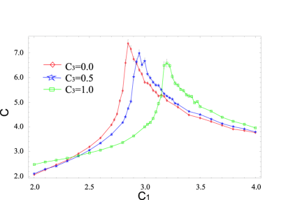
Figure 1: Specific heat for $L=24$ vs $c_{1}$ for fixed $c_{3}$. It exhibits a peak of AF transition at $c_{1}=2.8(2.95,3.25)$ for $c_{3}=0(0.5,1.0)$.

Let us next consider the role of the holon part $A_{\rm h}$. $A_{\rm h}$ comes from the hopping $t$ term in (2.1) and the parameter $c_{3}$ is expressed as in Eq.(2.18. The spinon-pair amplitude of $z_{x}$ and $z_{x+\mu}$ in $A_{\rm s}$ like $\tilde{z}_{x+\mu}\bar{z}_{x}$ measures the NN FM order of the original O(3) Heisenberg spins due to the relation,

$$|\bar{z}_{x+\mu}\cdot\tilde{z}_{z}|^{2}=\frac{1}{2}(1-\vec{S}_{x}\cdot\vec{S}_{x+\mu}).$$ (2.21)

Thus $A_{\rm h}$ favors both a FM coherent hopping amplitude, $\langle\bar{z}_{x+\mu}\tilde{z}_{x}\rangle$ and a BEC of $\phi_{x}$. In other words, a BEC of $\phi_{x}$ requires a short-range FM spin ordering.

III Numerical results I (3D model at finite $T$’s)

In this section we report the results of Monte Carlo simulations that we performed for the system given by Eqs.(2.9) and (2.10). We considered the cubic lattice with the periodic boundary condition with the system size (total number of sites) $V=L^{3}$ up to $L=30$, and used the standard Metropolis algorithm. The typical statistics was $10^{5}$ MC steps per sample, and the averages and errors were estimated over ten samples. The typical acceptance ratio was about $50$%. In the action we added a very small but finite ($\sim 10^{-7}$) external magnetic field.

Let us start with the region of relatively high $T$’s. In Fig.1 we show the specific heat per site $C$,

$$C=\frac{1}{V}\langle(A-\langle A\rangle)^{2}\rangle,$$ (3.1)

as a function of $c_{1}$ for several values of $c_{3}$. $C$ exhibits a peak that shifts to larger $c_{1}$ as $c_{3}$ is increased. This transition is nothing but the AF Néel phase transition observed previously for the $c_{3}=0$ caseTIM1 . Fig.1 and the relations (2.18) show that the Néel temperature is lowered by doped holes as we expected.

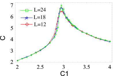
Figure 2: Size-dependence of the specific heat for $c_{3}=0.5$.

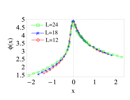
Figure 3: Scaling function $\phi(x)$ of (3.2) determined from the data of Fig.2.

In Fig.2 we present the system-size dependence of $C$ for $c_{3}=0.5$ in which the specific heat $C$ develops moderately but systematically as we increase $L$. We fitted this $C$ by using the finite-size scaling(FSS) of the form,

$$C(c_{1},L)=L^{\sigma/\nu}\phi(L^{1/\nu}\epsilon),$$ (3.2)

where $\epsilon=(c_{1}-c_{1c})/c_{1c}$ with the critical coupling $c_{1c}$ at infinite system size, and $\sigma,\;\nu$ are critical exponents. In Fig.3 we show the determined scaling function $\phi(x)$, from which we estimated the critical exponent of correlation length as $\nu=1.7$.

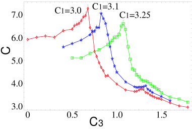
Figure 4: Specific heat for $L=24$ vs $c_{3}$ for fixed $c_{1}$. There are two peaks, which indicate the AF transition(in the smaller $c_{3}$-region) and the BEC transition (in the larger $c_{3}$ region).

In Fig.4 we present $C$ as a function of $c_{3}$ for fixed $c_{1}$. There exist two peaks in $C$. To study the origin of these peaks, we define the “specific heat” $C_{\rm s}$ and $C_{\rm h}$ for each term $A_{\rm s}$ and $A_{\rm h}$ of the action (2.10) separately as

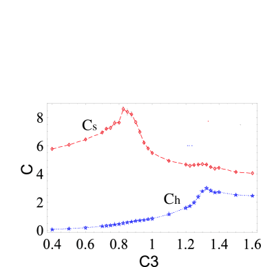
Figure 5: Specific heat $C_{\rm s}$ and $C_{\rm h}$ of (3.3) at $c_{1}=3.1$ and $L=24$. The location of peak of $C_{\rm s(h)}$ almost coincides the location of peak of $C$ in Fig.4 at smaller(larger) $c_{3}$.

$$C_{\rm s,h}=\frac{1}{V}\langle(A_{\rm s,h}-\langle A_{\rm s,h}\rangle)^{2}\rangle.$$ (3.3)

In Fig.5 we present $C_{\rm s}$ and $C_{\rm h}$ for $c_{1}=3.1$, in which $C_{\rm s}$ has a peak at $c_{3}\simeq 0.8$, the smaller-$c_{3}$ peak position of $C$ while $C_{\rm h}$ has a peak at $c_{3}\simeq 1.3$, the larger-$c_{3}$ position of $C$. From this result, we identify the peak at smaller $c_{3}$ expresses the AF transition in Fig.1, which is generated by $A_{\rm s}$, and the peak at larger $c_{3}$ expresses the BEC transition, which is driven by $A_{\rm h}$. Because each peak develops as $L$ is increased, they are both second-order phase transitions. The critical exponent of $C_{\rm s}$ of Fig.5 is estimated as $\nu=0.70$.

Let us turn to the low-$T$ (large-$c_{1}$) region and see what happens to the AF and BEC phase transitions. In Fig.6, we present $C$ for $c_{1}=6.0$. Again there exist two peaks but the order of them is interchanged. Both peaks develop as $L$ is increased, and therefore both of them are still second-oder phase transitions. As $c_{3}$ (or equivalently $\delta$) is increased, the transition into the BEC phase takes place first and then the AF phase transition follows. This means that there exists a phase in which both the AF and BEC long-range orders coexist.

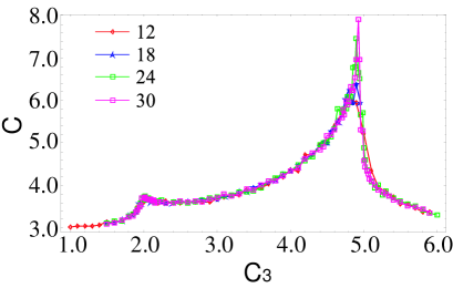
Figure 6: $C$ vs $c_{3}$ for $c_{1}=6.0$ with $L=12,18,24,30$. There exist again two peaks of AF and BEC phase transitions. However, their order are reversed (BEC peak in smaller $c_{3}$ and AF peak at larger $c_{3}$). Both peaks develop as $L$ is increased, supporting that they are of second order. In the region between the two peaks, the AF order and the BEC order coexist.

To verify the above conclusion, we measured the spin-spin correlation $G_{\rm AF}(r)$ of $\vec{S}_{x}$ and the correlation $G_{\rm BEC}(r)$ of the gauge-invariant “composite electron” pair variable $V_{x\mu}$ in each phase,

$$G_{\rm AF}(r) = {1\over 3V}\sum_{x,\mu}\langle\vec{S}_{x+r\mu}\cdot\vec{S}_{x}\rangle,$$ (3.4)

$$G_{\rm BEC}(r) = {1\over 12V}\sum_{x,\mu\neq\nu}\langle\bar{V}_{x+r\nu,\mu}V_{x\mu}\rangle+\mbox{c.c.},$$ (3.5)

$$V_{x\mu} \equiv \phi_{x+\mu}\phi_{x}\times\left\{\begin{array}[]{ll}z_{x+\mu}\bar{z}_{x},&\epsilon_{x}=1,\\ \bar{z}_{x+\mu}z_{x},&\epsilon_{x}=-1.\end{array}\right.$$ (3.8)

The results are shown in Figs.7 and 8. Fig.7 exhibits an interesting result in the coexisting phase of AF order and BEC at intermediate $c_{3}(\propto\delta)$. There the spin correlation has a FM component in the AF background. This shows that a short-range FM order is needed for the BEC as some mean-field theoretical studies of the $t$-$J$ modelmft indicate. As $c_{3}$ is increased further, the AF long-range order disappears and the FM order appears instead as a result of the holon-hopping amplitude. Fig.8 shows that the BEC certainly develops for larger $c_{3}$’s.

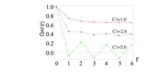
Figure 7: Spin-spin correlation function $G_{\rm AF}(r)$ of (3.4) in the three phases along $c_{1}=6.0$. For small $c_{3}$, $G_{\rm AF}(r)$ has a nonvanishing smooth component, i.e., the genuine AF staggered magnetization. (Remember the direction of the spin on the odd sites has been reversed.) For intermediate $c_{3}$, there appears an oscillatory, i.e., FM component in the AF background. For larger $c_{3}$, SC exists without AF long-range order, where the FM long-range order dominates.

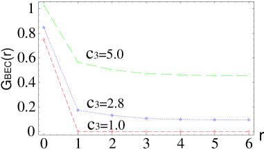
Figure 8: Correlation function $G_{\rm BEC}(r)$ (3.5) of bosonic hole(vacant electron) pair $V_{x\mu}$ in the three phases for $c_{1}=6.0$.

Let us comment here on the nature of BEC we have studied. To study BEC we have used $G_{\rm BEC}$, the long-range order of which implies a BEC of electron pairs. There may be another kind of BEC, a condensation of single bosonic electrons, which is measured by the electron-electron correlation function, $\langle\bar{B}_{x+r,\sigma}B_{x\sigma^{\prime}}\rangle$. (Note that $\langle\bar{\phi}_{x+r}\phi_{x}\rangle$ is not suitable because it is not gauge invariant and always vanishes.) However, as we have seen in Figs.4-6, there is only one peak at most in the specific heat apart from the peak representing the magnetic order, so the two condensations, one of single electrons and the other of pairs of electrons take place simultaneously.

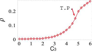
Figure 9: Monopole density $\rho$ for $c_{1}=6.0$ and $L=24$. Near the AF phase transition point at $c_{3}=4.8$ (with an arrow), the curvature of $\rho$ changes its sign.

We measured also the monopole density $\rho$TIM1 , which gives information on strongness of the fluctuation of the gauge field $U_{x\mu}$. In Fig.9 we present $\rho$ along $c_{1}=6.0$. $\rho$ changes its behavior around the AF transition point at $c_{3}=4.8$, indicating that the AF ordered phase corresponds to the deconfinement phase of $U_{x\mu}$. The low-energy excitations there are gapless spin waves described by the uncondensed component of $z_{x}$. In the paramagnetic phase, on the other hand, the confinement phase of $U_{x\mu}$ is realized and the low-energy excitations are the spin-triplet $\vec{S}_{x}$ with a gap.

To summarize the results of the 3D system, we present in Fig.10 the phase diagram in the $c_{3}/c_{1}-1/c_{1}$, i.e., $\delta-T$ plane. The Néel temperature decreases slowly as $\delta$ increases, while the BEC critical temperature develops rather sharply. The two orders can coexist at low $T$’s in intermediate region of $\delta$. Fig.10 has a close resemblance to the phase diagram of Ref.btj . However, in Ref.btj , the anisotropic spin coupling is considered and the phase separation occurs as a result. The coexistence phase of the AF and BEC orders obtained in Ref.btj is nonuniform and accompanied with this phase separation. In the present paper, we studied the system with the isotropic spin coupling, and the phase with both the AF and BEC orders is realized under the uniform distribution of holessu2 . In this sense, the model in the present paper is close to the fermionic $t$-$J$ model with parameters $t>J$sorella . We expect that the fermionic $t$-$J$ model has a similar phase diagram to Fig.10btJ2 . In Sec.6, we explain further the implication of the results obtained in the present paper to the phase structure of the fermionic $t$-$J$ model.

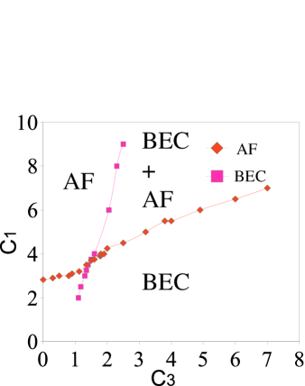
(a)

(b)

Figure 10: Phase diagram of the 3D model at finite $T$ in the $c_{3}-c_{1}$plane (a) and (b) in the $c_{3}/c_{1}-1/c_{1}$ plane ($c_{3}/c_{1}\propto t\delta/J$ and $1/c_{1}\propto T$). In the low-$T$ and intermediate $\delta$ region, there exists the coexisting phase of BEC and AF order. All the phase transition lines are of second order.

IV Bosonic $t$-$J$ model in the CP¹-Higgs representation: 2D model at $T=0$

As mentioned in Sect.1, the cold atoms can be put on a 2D optical lattice. At $T=0$ one may expect a BEC and/or magnetic ordering at certain conditions for density of atoms per well, interaction between atoms, etc. We expect that the bosonic $t$-$J$ model in the present section describes dynamics of bosonic atoms with (pseudo-)spin degrees of freedom and (strong) repulsive interactions between them. For the physics of high-$T_{\rm c}$ cuprates, it is also interesting to study the two-dimensional (2D) bosonic $t$-$J$ model at $T=0$. The main concern there is the quantum phase transitions (QPT) of magnetism, MIT, and SC. Study of the QPT in the doped CP¹ model is not only important for verifying the phase diagram at finite $T$ obtained in the above, but also interesting for physics of cold atom systems in optical lattices.

In this section, we shall briefly review the derivation of the effective field-theory model for the 2D fermionic $t$-$J$ model at $T=0$CP1 . Then, in this effective model, by replacing the fermionic holon variables by Higgs boson variables, we obtain the bosonic effective model of the 2D bosonic $t$-$J$ model at $T=0$. The main difference from the previous sections (the 3D model at finite $T$’s) is that the action contains the kinetic terms of spinons and holons due to their nontrivial $\tau$-dependence, and one should consider the 2+1 dimensional model. They are both 3D models but the couplings along the third-direction ($x_{3}$ or $\tau$) are different in the two models.

Let us start with the path-integral representation of the (quantum) partition function $Z_{\rm F}^{\rm 2D}$ of the 2D fermionic $t$-$J$ model in the slave-fermion representation with the CP¹ variablesCP1 ,

$$Z_{\rm F}^{\rm 2D}=\int\prod_{r,\tau}[d\psi_{r}(\tau)dz_{r}(\tau)]\exp\Big{(}A^{\rm 2D}_{\rm F}(\tau)\Big{)},$$ (4.1)

where $r=(x_{1},x_{2})$ denotes the site of the 2D lattice and $\tau\in(0,\infty)$ is the imaginary time. The action $A^{\rm 2D}_{\rm F}(\tau)$ is given byirrelevant

$$A^{\rm 2D}_{\rm F}(\tau) = \int_{0}^{\infty}d\tau\sum_{r}\Big{[}-\big{(}\bar{\psi}_{r}D_{r\tau}\psi_{r}+\bar{z}_{r}\partial_{\tau}z_{r}\big{)}$$ (4.2)

$$- t\sum_{i=1,2}\big{(}\bar{\psi}_{r}\bar{z}_{r+i}z_{r}\psi_{r+i}+\bar{\psi}_{r}\bar{z}_{r-i}z_{r}\psi_{r-i}\big{)}$$

$$- {J\over 4}\sum_{i}\bar{z}_{r}\vec{\sigma}z_{r}\cdot\bar{z}_{r+i}\vec{\sigma}z_{r+i}\Big{]},$$

$$D_{r\tau} \equiv \partial_{\tau}+iA_{r\tau},\ A_{r\tau}\equiv i\bar{z}_{r}\partial_{\tau}z_{r},$$ (4.3)

where $i=1,2$ denotes the spatial direction index and also the unit vector.

Each kinetic term, $\bar{\psi}_{r}D_{r\tau}\psi_{r}$, $\bar{z}_{r}\partial_{\tau}z_{r}$, in $A^{\rm 2D}_{\rm F}$ is purely imaginary, so the straightforward MC simulations cannot be applied. However, concerning to $\bar{z}_{r}\partial_{\tau}z_{r}$, by integrating out the half of the CP¹ variables (e.g., $z_{r}$’s on all the 2D odd sites, i.e., $\epsilon^{\rm 2D}_{x}\equiv(-)^{x_{1}+x_{2}}=-1$) one may obtain a purely real action as a result. That real action describes the low-energy spin excitations in a natural and straightforward manner.

Explicitly, we assume a short-range AF order,

$$(\bar{z}\vec{\sigma}z)_{r}\sim-(\bar{z}\vec{\sigma}z)_{r\pm i}.$$ (4.4)

Then we parameterize each CP¹ variable $z_{\rm o}$ at the 2D odd site o by referring to one of its NN partner $z_{\rm e}$ at the even site e at equal time as

$$z_{\rm o}=p_{\rm oe}z_{\rm e}+(1-|p_{\rm oe}|^{2})^{1/2}U_{\rm oe}\tilde{z}_{\rm e},$$ (4.5)

where $p_{\rm oe}$ is a complex number sitting on the link (oe) and $U_{\rm oe}$ is a U(1) phase factor that makes the parameterization (4.5) to be consistent with the local gauge symmetryvoe . The assumption (4.4) implies $|p_{\rm oe}|^{2}\ll 1$, which is justified by the $J$-term in the action (4.2) for the lightly doped case ($\delta\ll 1$)sraf . Integration over $z_{\rm o}$ is reduced to the integral over $p_{\rm oe}$, which may be approximated as the Gaussian integration link by link,

$$\int_{-\infty}^{\infty}d\bar{p}dp\exp(-\bar{p}Mp+\bar{p}k+\bar{\ell}p)$$

$$\ \ \ \propto{\rm det}M^{-1}\exp(\bar{\ell}M^{-1}k).$$ (4.6)

The CP¹ part of the resulting action is not symmetric concerning to spatial directions because the choice of a definite even-site partner breaks it. However, by considering the smooth configurations of spinons $z(r,\tau)$, one recovers the symmetric action in the form of continuum spaceacp1 ,

$$A_{{\rm CP}^{1}} = -{1\over 2a^{2}}\int_{0}^{\infty}d\tau\int d^{2}r$$

$$\times \Big{(}Ja^{2}\sum_{i=1,2}\overline{D_{i}z}D_{i}z+{1\over 2J}\overline{D_{\tau}z}D_{\tau}z\Big{)},$$

$$D_{\mu} \equiv \partial_{\mu}+iA_{\mu},\ A_{\mu}\equiv i\bar{z}\partial_{\mu}z,$$ (4.7)

where $a$ is the lattice spacing (hereafter we often set $a=1$). The relativistic couplings of (4.7) give rise to spin wave excitations in the background of AF order with the dispersion $E(k)\propto k$ instead of $E(k)\propto k^{2}$ in the FM spin model.

The integration over the odd-site spins affects the holon and spinon hopping term. The most important point is that the U(1) factor $U_{\rm oe}$ always appears in combination with $\psi_{\rm o}$ as $\bar{U}_{\rm oe}\psi_{\rm o}$, and therefore we redefine $\bar{U}_{\rm oe}\psi_{\rm o}\rightarrow\psi_{\rm o}$. Then new $\psi_{\rm o}$ transforms under a gauge transformation as $\psi_{\rm o}\rightarrow e^{-i\theta_{\rm e}}\psi_{\rm o}$. This property is consistent with the fact that spinon hopping amplitude, e.g., from even site (e’) to odd site (o), contains factor $(\tilde{z}_{\rm e}\cdot\bar{z}_{{\rm e}^{\prime}})$ in the resultant effective action like

$$(\tilde{z}_{\rm e}\cdot\bar{z}_{{\rm e}^{\prime}})\bar{\psi}_{\rm o}\psi_{{\rm e}^{\prime}}+\mbox{c.c.}$$ (4.8)

Finally, the holon kinetic term is now expressed by using $\psi_{\rm o}^{\rm new}=\bar{U}_{\rm oe}\psi_{\rm o}^{\rm old}$ aseta

$$-\int d\tau\left[\sum_{\rm e}\bar{\psi}_{\rm e}(\partial_{\tau}+iA_{{\rm e}\tau})\psi_{\rm e}+\sum_{\rm o}\bar{\psi}_{\rm o}(\partial_{\tau}-iA_{{\rm e}\tau})\psi_{\rm o}\right].$$

(4.9)

To proceed we note that the obtained total action is not symmetric w.r.t. the spatial directions, but a symmetric one can be available by reintroducing CP¹ variables at the 2D odd sites according to the invariance under a local U(1) gauge transformation. Furthermore, by choosing the lattice spacing in the $x_{3}$ direction suitably, the symmetry in all the three directions is recovered. Then the spin part $A^{\rm 2D}_{\rm s}$ of the action becomes nothing but the 3D action $A_{\rm s}$ of (2.10). Both of them have the same continuum limit (4.7) for the spin part, so they are to be categorized to the same universality class.

Then the bosonic $t$-$J$ model on the lattice is obtained by the replacement $\psi_{x}\rightarrow\sqrt{\mathstrut\delta}\phi_{x},\ \phi_{x}\equiv\exp(i\varphi_{x})$ as in Eq.(2.7). The partition function $Z^{\rm 2D}$ on the 2+1-dimensional spacetime lattice is then given by

$$Z^{\rm 2D} = \int\prod_{x}[dz_{x}d\phi_{x}\prod_{\mu}dU_{x\mu}]\exp(A^{\rm 2D}),$$

$$A^{\rm 2D} = A^{\rm 2D}_{\rm s}+A^{\rm 2D}_{\rm h},\ \ A^{\rm 2D}_{\rm s}=A_{\rm s}\ {\rm of\ Eq.}(\ref{action}),$$

$$A^{\rm 2D}_{\rm h} = {s_{3}\over 2}\Big{(}\sum_{x\in{\rm e}}\bar{\phi}_{x+3}U_{x3}\phi_{x}+\sum_{x\in{\rm o}}\bar{\phi}_{x+3}\bar{U}_{x3}\phi_{x}$$

$$+ \sum_{x\in{\rm e},i}\tilde{z}_{x+i}\bar{z}_{x}\bar{\phi}_{x+i}\phi_{x}+\sum_{x\in{\rm o},i}\tilde{z}_{x}\bar{z}_{x+i}\phi_{x+i}\bar{\phi}_{x}+{\rm c.c.}\Big{)}.$$

Here $x=(x_{1},x_{2},x_{3})$, and $r=(x_{1},x_{2})$ stands for the coordinates of the 2D plane and $x_{3}(=0,1,\cdots,\infty)$ is the discretized imaginary time ($\tau=x_{3}a_{3}$). Even (e) and odd (o) sites are defined regarding to the 2D plane as $\epsilon^{\rm 2D}_{x}\equiv(-)^{x_{1}+x_{2}}=1$(even), -1(odd).

The coefficients $c_{1},s_{3}$ are related to the parameters of the $t$-$J$ model as follows;c1s3

$$c_{1} \sim {\rm constant\ independent\ of}\ J\ {\rm and}\ t,$$

$$s_{3} \sim \frac{t}{J}\delta.$$ (4.11)

$c_{1}$ measures the solidity of the Néel state in the AF Heisenberg magnet at $T=0$. $s_{3}$ is the hopping amplitude of electrons. For the AF Heisenberg model with the standard NN exchange coupling, $c_{1}>c_{1c}\simeq 2.8$, and the critical value $c_{1c}$ decreases (increases) if long-range and/or anisotropic couplings that enhance (hinder) the AF order are addedYAIM .

In $A_{\rm h}$ we added the Hermitian conjugate of the holon kinetic term, $\bar{\phi}_{x+3}(\bar{U}_{x3},U_{x3})\phi_{x}$, which were absent in Eq.(4.9), to make the action real, explicitly. This modification might sound crucial. However, we expect it a modest replacement because the omitted imaginary part, $-i(\bar{\phi}_{x+3}U_{x3}\phi_{x}-$c.c.), etc, should have vanishing expectation value and behave mildly for the relevant configurations for the original action without the complex conjugates. Another support for this modification is given by taking into account the fluctuation of holon fieldrho .

Let us summarize the difference between the 2D model at $T=0$ and the 3D model at $T>0$ of (2.10). To see it explicitly, it is convenient to use the redefinition,

$$\phi_{x}^{\prime}\equiv\{\begin{array}[]{l}\bar{\phi}_{x}\ {\rm for}\ \epsilon^{\rm 2D}_{x}=-1\\ \phi_{x}\ {\rm for}\ \epsilon^{\rm 2D}_{x}=1\end{array}({\rm 2D\ model}),$$ (4.14)

and the relation $\bar{z}\tilde{z}^{\prime}=-\tilde{z}\bar{z}^{\prime}$. Then $A^{\rm 2D}_{\rm h}$ becomes

$$A^{\rm 2D}_{\rm h} = {s_{3}\over 2}\sum_{x}\Big{(}\bar{\phi}^{\prime}_{x+3}U_{x3}\phi_{x}^{\prime}$$ (4.15)

$$+ \sum_{i}\epsilon^{\rm 2D}_{x}\tilde{z}_{x+i}\bar{z}_{x}\phi_{x+i}^{\prime}\phi_{x}^{\prime}+{\rm c.c.}\Big{)}.$$

In the similar notation,

$$\phi_{x}^{\prime}\equiv\{\begin{array}[]{l}\bar{\phi}_{x}\ {\rm for}\ \epsilon_{x}=-1\\ \phi_{x}\ {\rm for}\ \epsilon_{x}=1\end{array}({\rm 3D\ model}),$$ (4.18)

the action $A_{\rm h}$ of the 3D model (2.10) is given as

$$A_{\rm h} = {c_{3}\over 2}\sum_{x,\mu}\Big{(}\epsilon_{x}\tilde{z}_{x+\mu}\bar{z}_{x}\phi_{x+\mu}^{\prime}\phi_{x}^{\prime}+{\rm c.c.}\Big{)}.$$ (4.19)

Thus, the hopping of holons $\phi_{x}$ along $\mu=3$ is uniform in the $\bar{\phi}\phi$-channel in the 2D model, while it is alternative in the $\phi\phi$-channel in the 3D model, i.e., the latter has an extra factor $(-)^{x_{3}}$.

V numerical results II (2D model at $T=0$)

V.1 Phase diagram

We studied the quantum system $A^{\rm 2D}$ of (IV) by MC simulationsmc3d . In this section we show the results of these calculations. Let us first present the obtained phase diagram in Fig.11. Its phase structure is globally similar to Fig.10 for the 3D model at finite $T$’s. As $s_{3}$ is increased, the AF order is destroyed and the BEC appears. The appearance of a first-order transition line is new. Below we shall see the details of various quantities, which support Fig.11. We select the following four points in the phase diagram to represent each of four phases;
(I) $s_{3}=1,c_{1}=2$; Normal and paramagnetic state.
(II) $s_{3}=1,c_{1}=20;$ AF state without BEC.
(III) $s_{3}=6,c_{1}=4$; BEC state with a FM order
(IV) $s_{3}=30,c_{1}=20$; AF and BEC state.
As presented later, various quantities are measured on these points and compared with each other.

(a)

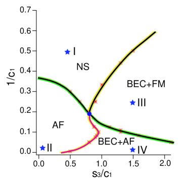
(b)

Figure 11: Phase diagram of the 2D $t$-$J$ model at $T=0$ in the $s_{3}-c_{1}$ plane (a) and (b) in the $s_{3}/c_{1}-1/c_{1}$ plane. The $c_{1}$-term controls the stability of the AF Néel order, whereas the $s_{3}$-term represents holon hopping. In the large-$c_{1}$ and intermediate $s_{3}/c_{1}$, there exists the coexisting phase of AF order and BEC. At the merging point of two transition lines, the peak in $C^{\rm 2D}$ disappears. NS stands for normal state and FM for ferromagnetic order. The phase transition line separating AF and BEC+AF phases is of first order, while other three transition lines are of second order. The four points (I-IV) marked by stars are selected as typical points: (I) $c_{1}=2,s_{3}=1;$ (II) $c_{1}=20,s_{3}=1;$ (III) $c_{1}=4,s_{3}=6;$ (IV) $c_{1}=20,s_{3}=30.$ 

Let us comment here on the assumption of the short-range AF order (4.4) in deriving the effective model (IV). As the phase diagram of Fig.11 shows, we find that there exists a FM order for small $c_{1}$ and large $s_{3}$. So the applicability of (4.4) in this parameter region might be questionable. However, the existence of the FM order itself in Fig.11 is consistent with the results of the 3D finite-$T$ system obtained in Secs.2,3 (as long as each phase at $T=0$ smoothly continues to $T>0$). Thus we expect that the global phase structure of Fig.11 is not affected by the assumption (4.4), although the location and the nature of the phase boundaries need some modifications. Furthermore, calculations of various physical quantities in that phase give us very important insight in understanding the whole phase structure of the model.

V.2 Specific heat and internal energy

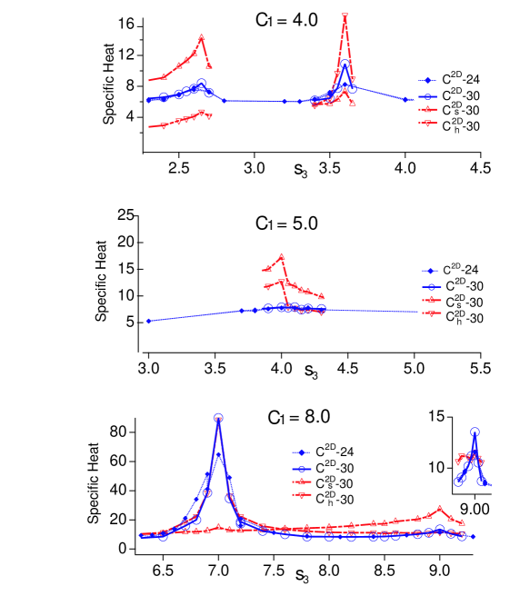
Figure 12: “Specific heats”, $C^{\rm 2D},C^{\rm 2D}_{\rm s},C^{\rm 2D}_{\rm h}$ vs $s_{3}$ for $c_{1}=4.0,5.0,8.0$. The notation $C_{\rm s}-24$ denotes $C^{\rm 2D}_{\rm s}$ for $L=24$, etc. At $c_{1}=5.0$ the two peaks almost merge.

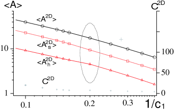
Figure 13: “Internal energies” $\langle A^{\rm 2D}\rangle,\langle A^{\rm 2D}_{\rm s}\rangle,\langle A^{\rm 2D}_{\rm h}\rangle$ vs $1/c_{1}$ for fixed $s_{3}/c_{1}=0.83$. We also show $C^{\rm 2D}$. The intersection point of the two phase transition lines (merging point of the AF and BEC phase transitions) is marked by an oval. At this region, $C^{\rm 2D}$ exhibits no anomalous behavior. Slightly anomalous behavior of $\langle A^{\rm 2D}_{\rm s}\rangle$ and $\langle A^{\rm 2D}_{h}\rangle$ cancel with each other and the total $\langle A^{\rm 2D}\rangle$ is a regular function of $1/c_{1}$.

We first study the “specific heat” (fluctuation of the action $A^{\rm 2D}$),

$$C^{\rm 2D}=\frac{1}{V}\langle(A^{\rm 2D}-\langle A^{\rm 2D}\rangle)^{2}\rangle.$$ (5.1)

In Fig.12 we present $C^{\rm 2D}$ as a function of $s_{3}$ for various values of $c_{1}$. We also present the “specific heats” $C^{\rm 2D}_{\rm s}$ and $C^{\rm 2D}_{\rm h}$ of each term $A^{\rm 2D}_{\rm s}$, $A^{\rm 2D}_{\rm h}$ in the action as defined in (5.1). As in the previous 3D finite-$T$ case, these results indicate that there exist two phase transition lines in the $s_{3}-c_{1}$ plane. They intersect at $c_{1}\simeq 5.0,s_{3}\simeq 4.0$. At the BEC transition points at high $c_{1}$’s (low $1/c_{1}$) (see Fig.12 for $c_{1}$=8.0 near $s_{3}\sim$7.0), $C^{\rm 2D}$ exhibits large values and large system-size dependence.

In order to see what happens at this intersecting point of the two phase transition lines, $c_{1}\simeq 5.0,s_{3}\simeq 4.0$, we measured “internal energies” $\langle A^{\rm 2D}\rangle,\langle A^{\rm 2D}_{\rm s}\rangle,\langle A^{\rm 2D}_{\rm h}\rangle$, and $C^{\rm 2D},\;C^{\rm 2D}_{\rm s},\;C^{\rm 2D}_{\rm h}$ as a function of $1/c_{1}$ along $s_{3}/c_{1}=0.83$. We show the result in Fig.13. At the intersection point, the total specific heat $C^{\rm 2D}$ exhibits no anomalous behavior, though $C^{\rm 2D}_{\rm s}$ and $C^{\rm 2D}_{\rm h}$ show peaks at that point. The calculations shown in Fig.13 show an interesting phenomenon that anomalous behavior in $\langle A^{\rm 2D}_{\rm s}\rangle$ and $\langle A^{\rm 2D}_{\rm h}\rangle$ cancel with each other and the total $\langle A^{\rm 2D}\rangle$ is a regular function of $1/c_{1}$.

To verify the order of the phase transitions, we measured distribution of $A^{\rm 2D}$ for configurations generated through the MC steps. In Fig.14 we present the distributions of $A^{\rm 2D}$ around $c_{1}=12,\;s_{3}=10,11,12$. The distribution at the middle point, $s_{3}=11$, shows a double-peak structure, so we concluded that the phase transition at this point is of first order. We found that the phase transition separating the AF and AF+BEC phases is of first order, while the other three transition lines are of second order. The difference of the order (1st vs. 2nd) in the 3D and 2D models may be attributed to the difference of holon hopping along the 3rd direction explained at the end of Sect.4. The present 2D model has a $\bar{\phi}\phi$ uniform coupling, which put more weight for ordering of holons and spinons than the 3D model. This may generate the first-order transition in certain regions.

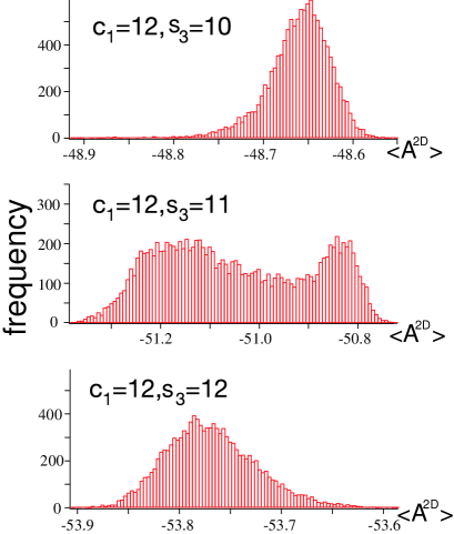
Figure 14: Distribution of $A^{\rm 2D}$. At $c_{1}=12,\;s_{3}=11$, it exhibits a double-peak structure, whereas the other two do not. This result means that the phase transition here is of first order.

V.3 Spin correlations

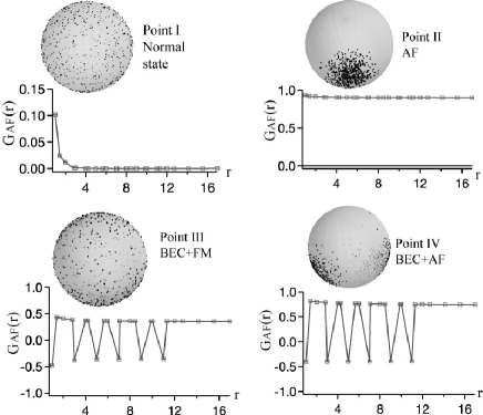
Figure 15: Spin correlation function $G_{\rm AF}(r)$ of (5.2) and spin snapshot at the points (I-IV) in Fig.11. (I) $c_{1}=2,\;s_{3}=1$. There is no long-range order of spins. (II) $c_{1}=20,\;s_{3}=1$. Endpoints of spins are centered near the south pole of the sphere, indicating the (AF) long-range order. (III) $c_{1}=4,\;s_{3}=6$. Results indicate the alternative order, i.e., the FM order. (IV) $c_{1}=20,\;s_{3}=30$. Endpoints form two groups on the sphere, indicating a canting “order” of spinsmft .

In this subsection, we investigate the spin correlation function at equal time,

$$G_{\rm AF}(r)\equiv\frac{1}{2V}\sum_{x,i}\langle\vec{S}_{x+ri}\vec{S}_{x}\rangle,$$ (5.2)

and show the snapshots of spin configurations. In Fig.15 we present $G_{\rm AF}(r)$ and the snapshots of spins at the typical four points (I-IV) in the phase diagrams of Fig.11. In the snapshots, each $\vec{S}_{x}$ starts from the center of the unit sphere and ends at a dot on the sphere.
(I) $c_{1}=2,s_{3}=1:$ Directions of spins are random, and there is no long-range magnetic order.
(II) $c_{1}=20,s_{3}=1:$ This point in the phase diagram is located in the deep AF region. It is obvious that there exists the AF long range order.
(III) $c_{1}=4,s_{3}=6:$ There appears the oscillative order around $G_{\rm AF}=0$, i.e., the FM long range order instead of the AF order.
(IV) $c_{1}=20,s_{3}=30:$ The even and odd site spins have their own magnetizations, $\vec{M}_{\rm e}$ and $\vec{M}_{\rm o}$, and these even and odd magnetizations cant with each other. This corresponds to the canting state studied in Ref.mft . In other word, there appear a component of a FM order in the background of AF long-range order.

V.4 Gauge dynamics and topological objects

In this subsection, we study the gauge dynamics associated with two U(1) gauge fields; the spin hopping amplitude $U_{x\mu}$ and the dual U(1) holon hopping amplitude $W_{xi}$ defined as follows;

$$W_{xi}\equiv\frac{\tilde{z}_{x}\bar{z}_{x+i}}{|\tilde{z}_{x}\bar{z}_{x+i}|}\in U(1).$$ (5.3)

For $U_{x\mu}$, we calculated the instanton density $\rho$ as in Sec.3instanton , whereas for $W_{xi}$, we calculated its gauge-invariant flux density,

$$f_{W}=\frac{1}{2\pi}\left<{\rm mod}\left[-i\log(\bar{W}_{x2}\bar{W}_{x+2,1}W_{x+1,2}W_{x1}),2\pi\right]\right>,$$

(5.4)

as $W_{xi}$ has only the spatial components. In Fig.16 we present $\rho$ and $f_{W}$ as functions of $s_{3}$; (a) $c_{1}=8.0$ and (b) $c_{1}=4.0$. For the both cases, it is obvious that $\rho$ and $f_{W}$ change their values suddenly at the relevant phase transition points determined by $C^{\rm 2D}$. We also verified that the singular behavior of the “specific heat” $C_{\rm s}\;(C_{\rm h})$ correlates to that of $\rho\;(f_{W})$ as it is expected.

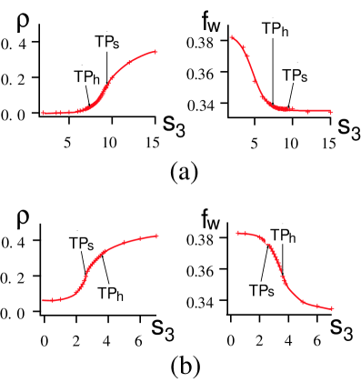
Figure 16: The instanton density $\rho$ and the flux density $f_{W}$ of (5.4) for (a) $c_{1}=8.0$ and (b) $c_{1}=4.0$. “TP_s”(“TP_h”) indicates the location of the AF (BEC) phase transition point. $\rho$ changes suddenly at TP_s. while $f_{W}$ changes suddenly at TP_h as expected.

$\rho$ influences the low-energy excitations of the spinon sector, whereas $f_{W}$ is related to the holon hopping. The large-$\rho$ region corresponds to the confinement phase of spinons and the low-energy excitations there are described by the spin-triplet $\bar{z}_{x}\vec{\sigma}z_{x}$. On the other hand, in the small-$\rho$ region of the AF state, deconfinement of quanta $z_{x}$ takes place, and the low-energy excitations are gapless spin waves.

Large fluctuations of $W_{xi}$ hinder coherent hopping of holons, and induce large fluctuations of the holon field $\phi_{x}$. However, as the holon density $\delta$ is increased, the holon hopping term stabilizes $W_{xi}$ and reduces $f_{W}$. From our study of $\rho$ and $f_{W}$, there seem to be some correlations between them, the origin of which is of course the term $A^{\rm 2D}_{\rm h}$.

V.5 Electron correlations

In this subsection, we study the correlation functions of single electrons and electron pairs in the 2D lattice in the various phases. We define the bosonic electron operator, ${\cal B}_{x\sigma}$, as follows;

$${\cal B}_{x\sigma}=\phi^{\dagger}_{x}\times\left\{\begin{array}[]{rl}z_{x\sigma},&\;\;{\rm for}\ \epsilon^{\rm 2D}_{x}=1,\\ \tilde{z}_{x\sigma},&\;\;{\rm for}\ \epsilon^{\rm 2D}_{x}=-1.\end{array}\right.$$ (5.5)

${\cal B}_{x\sigma}$ is invariant under the local U(1) gauge transformation. We define also operators of the spin-singlet and the spin-triplet pairs of bosonic electrons on the NN sites at equal time,

$$\Delta^{\rm s}_{xi}={\cal B}^{\dagger}_{x+i,\uparrow}{\cal B}^{\dagger}_{x\downarrow}-{\cal B}^{\dagger}_{x+i,\downarrow}{\cal B}^{\dagger}_{x\uparrow},$$

$$\Delta^{\rm t}_{xi}={\cal B}^{\dagger}_{x+i,\uparrow}B^{\dagger}_{x\uparrow}+B^{\dagger}_{x+i,\downarrow}B^{\dagger}_{x\downarrow}.$$ (5.6)

Then we introduce correlation functions of ${\cal B}_{x\sigma}$ and $\Delta^{\rm s,t}_{xi}$ at equal time as

$$G_{B}(r) \equiv \frac{1}{4V}\sum_{x,i,\sigma}\langle{\cal B}^{\dagger}_{x+ri,\sigma}{\cal B}_{x\sigma}\rangle,$$

$$G^{\rm s,t}(r) \equiv \frac{1}{2V}\sum_{x,i\neq j}\langle\bar{\Delta}^{\rm s,t}_{x+ri,j}\Delta^{\rm s,t}_{xj}\rangle.$$ (5.7)

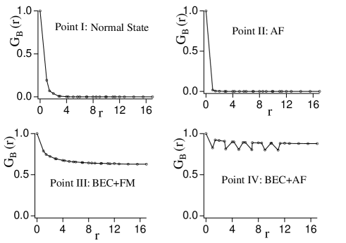
(a) Correlations of single electrons

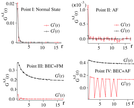
(b) Correlations of electron pairs

Figure 17: Electron correlation functions of (5.7) at the four points (I-IV) of Fig.11: (a) $G_{B}(r)$ of single bosonic electrons; (b) $G^{\rm s,t}(r)$ of spin-singlet and triplet pairs. Their meaning in each point is discussed in the text.

Their behaviors in the previous four points (I-IV) in Fig.11 are shown in Fig.17. Each point has the following properties;
(I) NS phase and (II) AF phase: All the three functions, $G_{B}(r),G^{\rm t,s}(r)$ have no long-range correlations.
(III) BEC+FM phase: $G_{B}(r)$ and the triplet pair $G^{\rm t}(r)$ exhibit the long-range order, and the BEC takes place in these channels.
(IV) BEC+AF phase: all the three functions exhibit the long-range order, and the BEC takes place.
As discussed in Sect.3, these results are consistent with the expectation that the two BECs, one of single electrons and the other of (triplet) electron pairs, take place at the same time. Furthermore, these results and the previous results on the (AF and FM) spin orders indicate that the BEC order and spin order can be superimposed in certain region. This is another example of the “spin-charge” separation.

VI Conclusion

In this paper, we have investigated the bosonic $t$-$J$ model in the CP¹-spinon + U(1) Higgs-holon representation. This model is introduced by replacing the fermionic holons with the bosonic ones in the slave-fermion $t$-$J$ model. We studied its phase structure and the dynamical properties both in the 3D finite-$T$ model and the 2D $T=0$ model. In particular, we are interested in the interplay of the BEC and AF order, because a coherent holon hopping is required for the BEC, whereas it hinders the AF long-range order. Our study by means of the MC simulations exhibits a phase diagram in which the coexistence region of AF and BEC orders appears. This result suggests that in the fermionic $t$-$J$ model a MIT takes place at a finite hole concentration $\delta_{c}$ and that phase transition point is located within the AF region of the spin dynamics. From the result of the present paper, we also expect that as $\delta$ is increased further, the BEC phase transition through the formation of electron pairs and their BEC takes place in the AF region. Actually, this problem can be studied in the framework of the fermionic $t$-$J$ model in the slave-fermion representation. Explicitly, one may obtain the effective model by integrating out the fermionic holon field by the hopping expansion. The resultant model includes only the bosonic variables; $z_{x}$ of spinons, “order parameter” of the coherent hopping of holons (i.e., the dual gauge field $W_{xi}$), and the SC order parameter of electron pairs, which can be analyzed numericallybtJ2 . For this scenario one should include some interaction terms that we have ignored in Sect.4 in our action, but have been generated in the process of integrating half of the spinon variablesCP1 . Among these terms, there is an attractive interaction between fermionic holons at NN sitesT0 . This term favors formation of holon pairs, and their coherent condensation gives rise to the superconductivity.

In an optical lattice, cold atoms at each well can have (pseudo-)spin degrees of freedom $2s+1=1,2,\cdots$, and there appears an AF interaction among them as a result of the repulsion. In this case, the CP¹ constraint is changed to $\sum_{a=1}^{2}|z_{xa}|^{2}=2s$, but this change of the normalization of $z_{x}$ can be absorbed by the parameter $c_{1}$. Then cold atom systems with one particle per well can be described by the CP¹ model like $A_{\rm s}$ of Eq.(2.10)so5 .

We expect that $A^{\rm 2D}$ of (IV) describes a 2D system of bosonic cold atoms with (pseudo-)spin and repulsive interaction in an optical lattice slightly away from the case of one-particle per well. For such system of cold atoms the phase diagram, Fig.11, indicates the coexistence of a BEC and a long-range order of an internal symmetry cold .

Let us comment on the effect of our replacement (2.7) of fermionic holons by Higgs field with a uniform amplitude, $\sqrt{\mathstrut\delta}\phi_{x}$. Being compared with the faithful bosonic model of the original $t$-$J$ model, this replacement certainly ignores fluctuations of the amplitude (density) of holon variable, which disfavors the BEC of holons. However, we expect that the BEC we obtained in the present model should survive in the faithful bosonic $t$-$J$ model, although location of the transition curves may change. This problem is under study and we hope that result will be reported in a future publicationNSIM .