Evolutionary Construction of Geographical Networks with Nearly Optimal Robustness and Efficient Routing Properties

Abstract

Robust and efficient design of networks on a realistic geographical space is one of the important issues for the realization of dependable communication systems. In this paper, based on a percolation theory and a geometric graph property, we investigate such a design from the following viewpoints: 1) network evolution according to a spatially heterogeneous population, 2) trimodal low degrees for the tolerant connectivity against both failures and attacks, and 3) decentralized routing within short paths. Furthermore, we point out the weakened tolerance by geographical constraints on local cycles, and propose a practical strategy by adding a small fraction of shortcut links between randomly chosen nodes in order to improve the robustness to a similar level to that of the optimal bimodal networks with a larger degree $O(\sqrt{N})$ for the network size $N$. These properties will be useful for constructing future ad-hoc networks in wide-area communications.

1 Introduction

Real complex networks, such as a power grid, an airline network, and the Internet, are embedded in a metric space, and long-range links are restricted [1, 2] for economical reasons. Moreover, there exists a common topological characteristic called scale-free(SF) that follows a power-law degree distribution $P(k)\sim k^{-\gamma}$, $2<\gamma<3$, which consists of many nodes with low degrees and a few hubs with high degrees. The SF structure is quite different from the conventional simple regular lattices and random graphs (also from more complicated graphs, e.g. the Voronoi or Delaunay diagrams [3]), and extremely vulnerable to intentional attacks on hubs [4]. By removing only about a few percent of high-degree nodes, a set of disconnected nodes leads to the global malfunction of a communication network [5]. Thus, the design of more robust networks than the SF structure, such as in the Internet or a Peer-to-Peer system, is important to reduce the threat of cyber-terrorism and of a natural disaster to communication infrastructures.

Recently, it has been analytically and numerically shown [6] that the robustness against both random and targeted removals of nodes is improved as the modality of degree is smaller in the multimodal networks with a specific type of degree distribution $P(k_{i})\propto a^{-(i-1)}$, $a>1$, $i=1,2,\ldots,m$: maximum modality, which include the SF structure as the largest modality with $m\rightarrow\infty$. Although the bimodal network with only two types of degree is the optimal in this class of networks under the assumption of uncorrelated tree-like structure, we can consider any other types of degree. Even with a small modality, the best allocation of degrees to nodes is generally unknown, and it may depend on the geographical positions of nodes. Clearly, in real communication networks, the position of node is not uniformly distributed [1] owing to the preference of crowded urbanism or geographical limitations on residences. Therefore, the spatial distribution is non-Poisson.

On the other hand, point processes give useful theoretical insights for the modeling of spatial distribution of nodes in wireless communication networks. Some mathematical approaches have been developed [7], while studying models other than e.g. the Poisson Voronoi tessellations and the Gibbs point process for a decomposition into some territories or other tessellation model for crack patterns [8] remains in an open and potential research field. In a different point process from the above models, we focus on the robustness of connectivity and on the efficiency of routing inspired by the progress in computer science and in complex network science [9, 10]. The topological structure and the traffic dynamics based on various routing protocols on complex networks have been studied actively to avoid the congestion of packets (e.g. see [11, 12, 13, 14]).

In addition, we are motivated by some geometric constructions of spatially grown SF networks [15, 16], in which newly added nodes and links are determined by the positions of already existing nodes. Our optimal policy is different from that in the growing complex networks by local linkings on a space [17, 18] in which the emergence of various topological structures is mainly discussed instead of the robustness of connectivity and the efficiency of routing. In computer science, geometric network models (e.g. Gabriel [19] and $\Theta$-graphs [20] in restricted power consumption) have also been proposed. Most of the research has been devoted to algorithmic and graph theoretical issues [21] about efficient routing and economical linking on a general (usually, uniformly random) position of node. However, percolation analysis in statistical physics should be included in the discussion, because the robust infrastructure on a realistic space and the routing scheme are closely related [19] in the design of network. The positions of nodes and the linkings strongly affect the distances of optimal paths and the tolerance of connectivity. Thus, by including the issues of routing and robustness, we consider how to design a communication network in realistic positions of nodes as base stations and linkings between them on a heterogeneously distributed population.

The organization of this paper is as follows. In Section 2, we introduce a new network construction according to a given distribution of a spatially heterogeneous population. We consider an incremental design of a communication network and a good property for decentralized routings. In Section 3, we numerically investigate the robustness of connectivity against both random failures and the intentional attacks on high degree nodes in the geographical networks. In particular, we point out a more weakened tolerance by geographical constraints on local cycles than the random null model under the same degree distribution, and propose a practical strategy to improve the tolerance by adding a small fraction of shortcuts. In Section 4, we summarize the results and briefly discuss the future studies.

2 Geographical network based on a population

We propose an evolutionary construction of geographical networks with good properties of small modality of degree, short distance path, and decentralized routing. The robustness of connectivity will be discussed in the later sections.

2.1 Geometric spanner

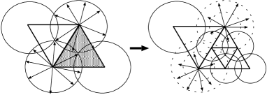
Let us consider the basic process of network evolution defined as follows. It is based on a point process for load balancing of incremental communication requests by stochastic subdivisions of a triangle. Each node of the triangle corresponds to a base station for transferring messages and the link between them corresponds to a wireless or wired communication line, however the technical details to distinguish them at the physical device level is beyond our current scope of network modeling.

Step0:

Set an initial triangulation of any polygonal region which consists of equilateral triangles.

Step1:

At each time step, a triangle is chosen with a probability proportional to the population (by summing up the number of people) in the corresponding space.

Step2:

Then, as shown in Figs. 1(a) and 2(a), four smaller triangles are created by adding facility nodes at the intermediate points on the communication links of the chosen triangle. This procedure is for a division of the service area.

Step3:

Return to Step 1.

(a) Re-assignment to nodes

(b) Regulation of communication range

Figure 1: Basic division process. (a) Re-assignment of communication requests to nodes as the nearest base stations. The arrows indicate the directions for transfered requests from users in the area. (b) Power of orientative wireless beam regulated by the subdivision. Each circle represents the range.

(a) Subdivision

(b) Example

Figure 2: (Color online) Heterogeneous network configuration. (a) Subdivision from a shaded triangle in an initial hexagon at left into four smaller triangles at right. The dashed circle represents the range of a wireless beam from each node. (b) Example of a network on the Fukui-Kanazawa area in Japan. From light (yellow) to dark (red) color, the gradation is proportionally assigned to the population in each block. Note that the white areas at the upper left and the lower right are the sea of Japan and the Hakusan mountain range, respectively.

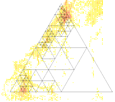
In the subdivision of this network, we use a mesh data of population statistics ($8^{2}\times 10^{2}\times 4=25600$ blocks for $80km^{2}$ in the Fukui-Kanazawa area, provided by Japan Statistical Association), and recalculate the mapping between the blocks and each triangle to count the number of people in the triangle space. It is natural that the amount of communication requests depends on the activities of people, therefore are estimated to be proportional to the population in the area. We consider such a stochastic construction of geographical networks for the general discussion, however a deterministic evolutionary construction is also possible when the population inside the corresponding triangle locally accesses a certain threshold. We mention that, in the meaning of practical construction, the subdivision is generated in a distributed manner according to the increase of communication requests in individual areas. The detailed procedures depend on technological issues in wide-area wireless communications.

According to the population, an example of randomly constructed network with a total number of nodes $N=100$ is shown in Fig. 2(b). This configuration resembles a heterogeneous random version of a Sierpinski gasket. For any population, since it has a small modality with the trimodal degrees: $k_{1}=2$ (or $3$ for the initial hexagon), $k_{2}=4$, and $k_{3}=6$ grown from the initial triangle, a highly tolerant connectivity may be expected from Ref.[6] because of the small modality of degree. Note that the smallest degree $k_{1}$ is fixed on the initial nodes with the existing probability $p_{1}=3/N$ (or $6/N$ for the initial hexagon) in this rule of geographical network generation, while in the optimal bimodal networks, $k_{1}$ with the probability $p_{1}=1-p_{2}$ is uniformly determined by $k_{2}=\sqrt{\langle k\rangle N}$, $p_{2}=\left(\frac{A^{2}}{\langle k\rangle N}\right)^{3/4}$ and $A=\{\frac{2\langle k\rangle^{2}(\langle k\rangle-1)^{2}}{2\langle k\rangle-1}\}^{1/3}$ under the assumption of an uncorrelated tree-like structure of large random networks for $N\gg 1$, then $k_{2}\gg 6$ is obtained. Here, $\langle k\rangle$ denotes a given average degree. Since the differences are not only the number of modalities but also the size of largest degree, the robustness should be carefully discussed. We will numerically compare the robustness in the optimal bimodal networks with that in our proposed geographical networks under the same $\langle k\rangle$ at the end of next section.

On the other hand, as a good graph property known in computer science, the proposed network becomes the $t$-spanner [22] with a maximum stretch factor $t=2$, since the equilateral property holds in spite of various sizes of the triangle. In other words, the network consists of the fattest triangles, then the length of the shortest distance path between any nodes $u$ and $v$ is bounded by $t$ times the direct Euclidean distance $d(u,v)$. Since narrow triangles as in random Apollonian networks [16] constructed by different geometric subdivisions from ours give rise to a long distance path, such a construction does not provide a suitable topology for routing paths with as short distances as possible. In other geometric graphs, the stretch factor becomes larger: $t=2\pi/(3cos(\pi/6))\approx 2.42$ for Delaunay triangulations [23] and $t=2\alpha\geq 4\sqrt{3}/3\approx 2.3094$ for two-dimensional triangulations with an aspect ratio of hypotenuse/height less than $\alpha$ [19] whose lower bound is given for the triangulation lattice that consists of the fattest equilateral triangles. Although $\Theta$-graphs [20] with $K$ non-overlapping cones have $t=1/(\cos(2\pi/K)-\sin(2\pi/K))\rightarrow 1$ asymptotically as $K\rightarrow\infty$, a large amount of $O(KN)$ links is necessary, and the links may be crossed (as non-planar) and give rise to interferences between wireless beams. In general graphs, even the existence of a bounded stretch factor is uncertain.

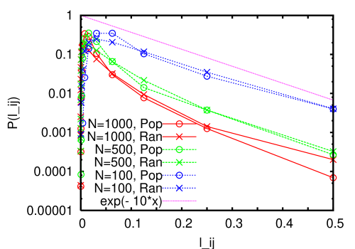
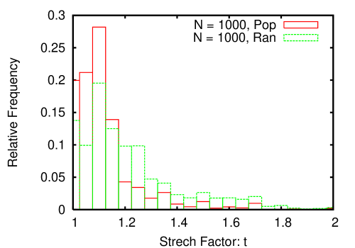
Figure 3 shows typical cases of the stretch factor on the shortest distance path in our model. We numerically investigate the distributions of the link length and of the stretch factor as shown in Fig. 4. Many paths connected by the majority of short links have small stretch factors. The average link lengths $\bar{l}_{ij}$ are less than half of the initial link length normalized with refer to the biggest triangle, as $0.057$ for $N=100$ and $0.014$ for $N=1000$ in the Pop ($\bar{l}_{ij}=0.05$ for $N=100$ and $0.01$ for $N=1000$ in the Ran), the average factors $\bar{t}$ are small as $1.1512$ for $N=100$ and $1.1395$ for $N=1000$ ($\bar{t}=1.2008$ for $N=100$ and $1.2297$ for $N=1000$ in the Ran). Thus, our proposed networks have good properties regarding path distance.

Figure 3: Typical cases of the stretch factor: (a) $t=2\sqrt{3}/3\approx 1.15$, (b) $t=\sqrt{3}\approx 1.73$, and the maximum (c) $t=2$. The dashed line is the shortest distance path between the source and the terminal nodes marked by circles. Note that all the triangles of different sizes are equilateral in the configuration.

(a) Dist. of Link Length

(b) Histogram of t-value

Figure 4: (Color online) Distance properties of the geographical networks with sizes $N=100\sim 1000$ according to the population in Fig. 2(b) and the uniformly random choice of a triangle corresponded to the case of a general population. These cases are denoted as abbreviations by Pop and Ran, respectively. (a) The distribution $P(l_{ij})$ of the link length $l_{ij}$ decays nearly exponentially, as shown by the magenta line defined by $\exp(-10\;l_{ij})$. (b) High frequencies are observed for small stretch factors $t<1.2$, while low frequencies for large ones which are bounded by $t=2$.

2.2 Decentralized face routing

For ad-hoc networks, a routing protocol should be simple to reduce energy consumption in keeping the reachability. However some of the routing schemes in early work lead to the failure of guaranteed delivery [24], e.g., in the flooding algorithm multiple redundant copies of a message are sent and cause network congestion, while greedy and compass routings may occasionally fall into infinite loops. On the other hand, except for some class of graphs, it is costly to seek the shortest path for a map in which connections are unknown in advance.

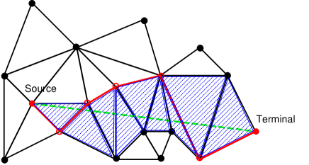
Fortunately, since the proposed geographical networks belong to a special class of graph which is planar and consists of convex (equilaterally triangular) faces, we can apply the efficient decentralized algorithm [25] that guarantees the delivery of a message using only local information based on the positions of the source, the terminal nodes, and the adjacencies of the current node on a path. In recent technologies, the positions are measured by means of a GPS or other methods, then the reachable path to a terminal node $Te$ can be found in a proper mixing of upper and lower chains extracted from the edges of the faces as shown in Fig. 5. Without multiple copies of the message, the next forwarding node from each node on the upper and lower chains is determined only by the positions of adjacent nodes and the distance from a source node $So$. In this class, with the property of routing called competitive, the length of the routing path is bounded in a constant factor to that of the shortest path and also to the distance $d(So,Te)$ on the straight line because of the $t$-spanner.

This competitive algorithm [25] or a combination by greedy and face routings in asymptotically (at the lower bound) worst-case optimal traveling on a general planar network [26] acts in a decentralized manner, therefore a global information such as the static routing table in the Internet’s TCP/IP protocol is not necessary. Moreover, these algorithms can be extended (see the Appendix of [28] and a related idea [27]) to add a small fraction of shortcuts discussed in the next section. We emphasize that such geographical protocols are not only successfully used for message delivery in social friendships [29] but are also very promising for constructing wireless networks with a higher efficiency and scalability in a dynamic environment [30].

Figure 5: (Color online) Efficient face routing on a planar network. The (red) reachable shortest path through the nodes marked by open circles between the source and the terminal nodes can be found from the edges of the (blue) shaded faces that intersect the (green) dashed straight line. The two paths on the edges above and below the line are the upper and the lower chains, respectively.

3 Numerical robustness analysis

We aim to maximize the sum of critical fractions $f_{T}=f_{r}+f_{t}$ to be optimal network against both random failures and targeted attacks on nodes with large degrees as robust as possible on a spatially heterogeneous distribution of population. Here, $f_{r}$ and $f_{t}$ denote the critical fractions of these damages at the breaking of the giant component (GC).

For a preliminary, we numerically estimate the total numbers of nodes $N(\tau)$ and links $M(\tau)$ at time step $\tau$ over 100 realizations of the geographical network. They grow as $N(\tau)=N(0)+2.35\tau$ and $M(\tau)=M(0)+5.34\tau$, where $N(0)=6$ and $M(0)=9$ for the initial triangle (or $N(0)=7$ and $M(0)=12$ for the initial hexagon). Thus, in the subdivision, two or three nodes per step are added with a high frequency, and the average degree is $\langle k\rangle=2M(\tau)/N(\tau)\approx 4.54$. Since the total link $\langle k\rangle N/2$ is more than twice that of $N-1$ links on a tree of $N$ nodes, there possibly exist many cycles.

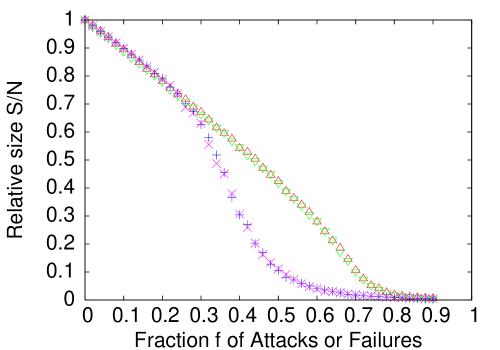
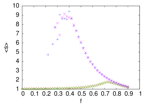
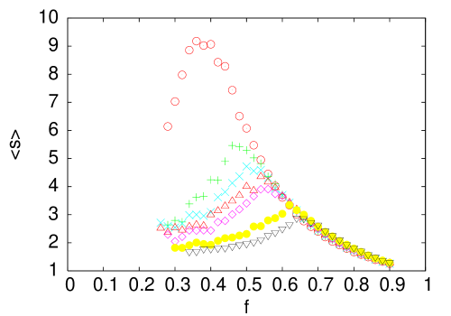
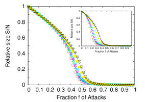
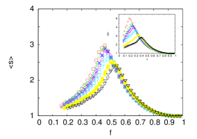
As the simulation result for the removals, Fig. 6 indicated with blue $+$ and magenta $\times$ marks show that the size $S$ of the GC rapidly decreases at the fraction $f\approx 0.4$. A similar vulnerability caused by geographical constraints on local cycles has been found in a family of SF networks embedded in a planar space [31] and SF networks on a lattice [32]. To clearly see the effect of constraints, we investigate the non-geographical rewired versions under the same degree distribution (of course with the same average degree $\langle k\rangle$). In the rewiring [33], two pairs of nodes at the ends of randomly chosen links are exchanged in holding the degree of each node. Therefore, the geographical constraints are entirely reduced. In general, the rewired version of a network is the null model that depend only on the degree distribution ignoring the other topological structures: cycles, degree-degree correlation, fractal or hierarchical substructure, diameter of graph, etc. The red $\bigtriangleup$ and green $\bigtriangledown$ marks shown in Fig. 6 indicate that the critical fractions at the peak of $\langle s\rangle$ increases to $f_{r}\approx 0.7$ and $f_{t}\approx 0.6$. Such improvement of the robustness is consistent with the result obtained for the geographical SF networks [31].

(a) Giant Component

(b) Isolated Clusters

Figure 6: (Color online) Comparison of the geographical and the non-geographical rewired networks at $N=1000$. (a) Relative size $S/N$ of the GC after the removal of nodes. The plus(blue) and cross(magenta) marks indicate the corresponding results for the geographical networks against random failures and intentional attacks. The upper triangle(red) and down triangle(green) marks indicate the corresponding results for the non-geographical rewired versions against them, respectively. (b) Average size $\langle s\rangle$ of isolated clusters except the GC. The peak indicates the critical point at which the whole connectivity breaks. Each point is obtained from the average over 100 realizations of the geographical network constructed from the initial triangle ($\times$ 100 samples of random rewirings).

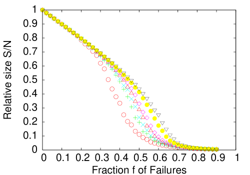
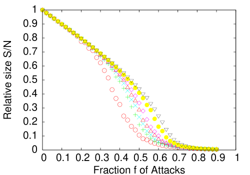
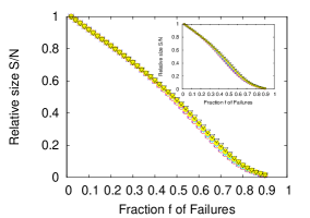
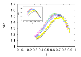
Although the full rewiring is better in terms of the robustness, it completely ignores the positions of nodes and the distances of links. As another practical strategy, it is expected that adding a small fraction of shortcuts between randomly chosen nodes has a similar effect to the rewiring [28]. Indeed, Figs. 7 and 8 show the improvement of robustness against both random failures and intentional attacks. As the shortcut rate marked from red $\bigcirc$ to black $\bigtriangledown$ increases, a larger GC remains, and the breaking point at the peak of $\langle s\rangle$ shifts to a larger fraction $f$ of the removal. Only about 10 % of the adding reaches a similar level of $f_{r}\approx 0.7$ or $f_{t}\approx 0.6$ in the non-geographical rewired version (compare with Fig. 6 indicated with $\bigtriangleup$ and $\bigtriangledown$ marks). In addition, the finite effect on the critical fractions is very small as shown in Table 1, however it has occurred that the positioning of the node is inaccurate written a round-off error in the very dense case of $N=10^{5}$, especially for $0\%$ shortcuts.

We compare the above results shown in Figs. 7 and 8 with the robustness of the optimal bimodal network [6] defined by $k_{2}=\sqrt{\langle k\rangle N}=67.38$ and $p_{2}=\left(\frac{A^{2}}{\langle k\rangle N}\right)^{3/4}=0.01445$ for $N=1000$ and $\langle k\rangle=4.54$. Since the degree and the number of nodes for each type of degree must be an integer, the appropriate combination is $k_{2}=67$ or $68$, $p_{2}=0.014$ or $0.015$, $k_{1}=(\langle k\rangle-k_{2}p_{2})/p_{1}=4$ or $3$, and $p_{1}=1-p_{2}=0.986$ or $0.985$; then, $\langle k\rangle=3.975$ or $4.882$ is the closest to the value $4.54$ in our geographical networks. On the two pairs of degree distributions, the bimodal networks are randomly constructed by full rewirings from an initial configuration. As shown in Figs. 9 and 10, the critical fractions $f_{r}$ and $f_{t}$ are slightly larger around $0.4\sim 0.7$, however the effect of shortcuts barely works and is weaker than that in our geographical networks.

(a) Giant Component

(b) Isolated Clusters

Figure 7: (Color online) Damages by random failures in the geographical networks and the shortcut versions at $N=1000$. (a) Relative size $S/N$ of the GC. The open circle(red), plus(green), cross(cyan), upper triangle(orange), diamond(magenta), closed circle(yellow), and down triangle(black) marks indicate the corresponding results for the shortcut rate of 0, 3, 5, 7, 10, 20, and 30 %, respectively. (b) Average size $\langle s\rangle$ of isolated clusters except the GC. Each point is obtained from the average over 100 realizations of the geographical network constructed from the initial triangle $\times$ 100 samples of random shortcuts.

(a) Giant Component

(b) Isolated Clusters

Figure 8: (Color online) Damages by intentional attacks in the geographical networks and the shortcut versions at $N=1000$. (a) Relative size $S/N$ of the GC. (b) Average size $\langle s\rangle$ of isolated clusters except the GC. The marks are the same as in Fig. 7. Each point is obtained from the average over 100 realizations of the geographical network constructed from the initial triangle $\times$ 100 samples of random shortcuts.

Shortcut		$f_{r}$				$f_{t}$
Rate %	$N=10^{2}$	$10^{3}$	$10^{4}$	$10^{5}$	$N=10^{2}$	$10^{3}$	$10^{4}$	$10^{5}$
0	0.352	0.348	0.386	0.058	0.351	0.335	0.384	0.100
3	0.474	0.443	0.499	0.469	0.469	0.481	0.425	0.468
5	0.529	0.501	0.542	0.502	0.509	0.499	0.540	0.503
7	0.525	0.537	0.554	0.538	0.520	0.525	0.503	0.535
10	0.545	0.542	0.566	0.568	0.568	0.552	0.571	0.565
20	0.600	0.605	0.627	0.639	0.619	0.596	0.635	0.638
30	0.646	0.641	0.671	0.682	0.651	0.641	0.663	0.680
Rewired	0.726	0.722	0.703	0.687	0.718	0.736	0.699	0.690

Table 1: Critical fractions $f_{r}$ and $f_{t}$ at the peak of $\langle s\rangle$ are consistent for different sizes $N$ of the geographical networks with shortcuts and the rewired versions. Each value is obtained from the average over 100 realizations of the geographical network constructed from the initial triangle $\times$ 100 samples of random shortcuts and rewirings.

(a) Giant Component

(b) Isolated Clusters

Figure 9: (Color online) Damages by random failures in the optimal bimodal networks and the shortcut versions at $N=1000$ with the over-estimated $\langle k\rangle=4.882>4.54$, $k_{1}=4$, and $k_{2}=67$. (a) Relative size $S/N$ of the GC. (b) Average size $\langle s\rangle$ of isolated clusters except the GC. Insets show the results with the under-estimated $\langle k\rangle=3.975<4.54$, $k_{1}=3$, and $k_{2}=68$. Each point is obtained from the average over 100 realizations $\times$ 100 samples of random shortcuts. The marks are the same as in Fig. 7.

(a) Giant Component

(b) Isolated Clusters

Figure 10: (Color online) Damages by intentional attacks in the optimal bimodal networks and the shortcut versions at $N=1000$ with the over-estimated $\langle k\rangle=4.882>4.54$, $k_{1}=4$, and $k_{2}=67$. (a) Relative size $S/N$ of the GC. (b) Average size $\langle s\rangle$ of isolated clusters except the GC. Insets show the results with the under-estimated $\langle k\rangle=3.975<4.54$, $k_{1}=3$, and $k_{2}=68$. Each point is obtained from the average over 100 realizations $\times$ 100 samples of random shortcuts. The marks are the same as in Fig. 7.

4 Conclusion

According to spatially distributed communication requests based on a given population density, we have proposed an evolutionarily constructed geographical network by the iterative division of equilateral triangles. Through the numerical simulation for investigating the robustness, the obtained results are summarized as follows. We note that they are consistent with other results on population densities besides the example of Fig. 2(b), e.g. for the the geographical networks generated by the iterative choice of a triangle with a uniformly random probability, the robustness is similar to that in Figs. 6-8.

• The proposed networks have suitable properties of short paths as the $t$-spanner [22] and efficient decentralized routing [25] for wireless communications. Moreover, the incremental construction can be implemented to accommodate a growing activity or population.

• To improve the vulnerability caused by the geographical constraints [31, 32], we have considered a practical strategy by adding a small fraction of shortcuts between randomly chosen nodes [28], and numerically confirmed the effect.

• The degree distribution becomes trimodal at most without hub nodes, the robustness of the connectivity is slightly weak but is maintained as similar level as the optimal bimodal networks with a larger maximum degree [6].

These results are useful for the design of ad-hoc networks with efficiency, scalability, and tolerance of connectivity in wide-area communications.

Since our trimodal model has a maximum degree that is not extremely large compared to other degrees, instead of hub attacks, a spatial cutting into several dense parts by removing a small number of nodes on lines of large triangles may be considerable. Even in such cases, we expect that shortcuts effectively work to bridge isolated clusters by the removals. More detailed analysis is the subject of future study that includes how to find the structural vulnerable points. Other important issues are the development of routing schemes taking into account the structure layered by the size of the triangle, the analysis of traffic dynamics with the phase transition between free flow and congestion according to the forwarding capacity at a node and queue discipline (FIFO etc.), and considering various optimal policies in matching application requirements.

References

- [1] S.-H. Yook, H. Jeong, and A.-L. Barabási, PNAS, 99(21), 13382, (2002).
- [2] M.T. Gastner, and M.E.J. Newman, Eur. Phys. J. B, 49(2), 247, (2006).
- [3] A. Okabe, B. Boots, K. Sugihara, and S.N. Chiu, Spatial Tessellations, 2nd ed., John Wiley, 2000.
- [4] R. Albert, and A.-L. Barabási, Nature, 406, 378, (2000).
- [5] R. Pastor-Satorras, and A. Vespignani, Evolution and Structure of the Internet, Cambridge University Press, 2004.
- [6] T. Tanizawa, G. Paul, S. Havlin, and H.E. Stanley, Phys. Rev. E, 74, 016125, (2006).
- [7] B. Blazsczyszyn, and R. Schott, Japan J. Ind. Appl. Math., 22(2), 179, (2005).
- [8] W. Nagel, J. Mecke, J. Ohser, and V. Weiss, The 12th Int. Congress for Stereogy, (2007). http://icsxii.univ-st-etiene.fr/Pdfs/f14.pdf
- [9] A.-L. Barabási, LINKED: The New Science of Networks, Perseus, Cambridge, MA, 2002.
- [10] M. Buchanan, NEXUS: Small Worlds and the Groundbreaking Science of Networks, W.W.Norton, New York, 2002.
- [11] L. Zhao, Y.-C. Lai, K. Park, and N. Ye, Phys. Rev. E, 71, 026125, (2005).
- [12] G. Yan, T. Zhou, B. Hu, Z.-Q. Fu, and B.-H. Wang, Phys. Rev. E, 73, 046108, (2006).
- [13] W.-X. Wang, B.-H. Wang, C.-Y. Yin, Y.-B. Xie, and T. Zhou, Phys. Rev. E, 73, 026111, (2006).
- [14] S. Sreenivasan, R. Cohen, E. Lórez, Z. Toroczkai, and H.E. Stanley, Phys. Rev. E, 75, 036105, (2007).
- [15] J.P.K. Doye, and C.P. Massen, Phys. Rev. E, 71, 016128, (2005).
- [16] T. Zhou, G. Yan, and B.-H. Wang, Phys. Rev. E, 71, 046141, (2005).
- [17] Y.-B. Xie, T. Zhou, W.-J. Bai, G. Chen, W.-K. Xiao, and B.-H. Wang, Phys. Rev. E, 75, 036106, (2007).
- [18] R. Xulxi.-Brunet, and I.M. Sokolov, Phys. Rev. E, 75, 046117, (2007).
- [19] E. Kranakis, and L. Stacho, In Handbook of Algorithms for Wireless Networking and Mobile Computing, edited by A. Boukerche, (Chapman & Hall/CRC, 2006), Chap. 8.
- [20] M. Farshi, and J. Gudmundsson, Proc. of the 13th European Symposium on Algorithms, edited by G.S. Brodal and S. Leonardi, ESA 2005, LNCS, 3669, 556, (2005).
- [21] X.-Y. Li, Wireless Computing and Mobile Computing, 3, 119, (2003).
- [22] M.I. Karavelas, and L.J. Guibas, Proc. of the 12th ACM-SIAM Symposium on Discrete Algorithms, (2001).
- [23] J.M. Keil, and C.A. Gutwin, Discrete and Computational Geometry, 7, 13, (1992).
- [24] J. Urrutia, In Handbook of Wireless Networks and Mobile Computing, edited by I. Stojmenović, (John Wiley & Sons, 2002), Chap. 18.
- [25] P. Bose, and P. Morin, Theoretical Computer Science, 324(2-3), 273, (2004).
- [26] F. Kuhn, R. Wattenhofer, and A. Zollinger, Proc. of the 4th ACM International Workshop on Mobile ad hoc Networking and Computing, (MObiHOc’03), pp.267-278, (2003),
- [27] F. Kuhn, R. Wattenhofer, and A. Zollinger, Proc. of the 6th International Workshop on Discrete Algorithms and Methods for Mobile Computing and Communications, (DialM’02), pp.24-33, (2002).
- [28] Y. Hayashi, and J. Matsukubo, Physica A, 380, 552, (2007).
- [29] D. Liben-Nowell, J. Novak, R. Kumar, P. Raghaven, and A. Tomkins, PNAS, 102, 11623, (2005).
- [30] K. Seada, and A. Helmy, In Handbook of Algorithms for Wireless Networking and Mobile Computing, edited by A. Boukerche, (Chapman & Hall/CRC, 2006), Chap. 15.
- [31] Y. Hayashi, and J. Matsukubo, Phys. Rev. E, 73, 066113, (2006).
- [32] L. Huang, L. Yang, and K. Yang, Europhys. Lett., 72(1), 144, (2005).
- [33] S. Maslov, K. Sneppen, and A. Zaliznyak, Physica A 333, 529, (2004).