Probing condensate order in deep optical lattices

Abstract

We study interacting bosons in optical lattices in the weak-tunneling regime in systems that exhibit the coexistence of Mott-insulating and condensed phases. We discuss the nature of the condensed ground state in this regime and the validity of the mean-field treatment thereof. We suggest two experimental signatures of condensate order in the system. (1) We analyze the hyperfine configuration of the system and propose a set of experimental parameters for observing radio-frequency spectra that would demonstrate the existence of the condensed phase between Mott-insulating phases. We derive the structure of the signal from the condensate in a typical trapped system, taking into account Goldstone excitations, and discuss its evolution as a function of temperature. (2) We study matter-wave interference patterns displayed by the system upon release from all confining potentials. We show that as the density profiles evolve very differently for the Mott-insulating phase and the condensed phase, they can be distinguished from one another when the two phases coexist.

I Introduction

Ultracold bosons in optical lattices allow extensive studies of quantum phases of condensed matter in controlled environments Greiner03 ; Bloch08 . When the tunneling energy, relative to the interaction energy, decreases across a critical value, the system undergoes a transition from the superfluid phase to the Mott-insulating phase Fisher89 . This transition has been observed in experiments by imaging matter wave interference patterns of the system Greiner02 . In realistic systems, a confining trap renders the density of bosons non-uniform and, in a sufficiently deep optical lattice (where the lattice depth is over 20 times the recoil energy), this inhomogeneous system is predicted to have a multiple-layer structure in which Mott-insulator layers having different occupation number are separated by relatively thin condensate layers Jaksch98 ; DeMarco05 . The study of such inter-layer condensates is important for a variety of reasons. From the perspective of quantum information schemes Rabl03 ; Jaksch05 ; Popp06 , robust, high-fidelity Mott-insulator states are required and the presence of a condensate is in fact a hindrance. The condensate is also of interest in and of itself; its ground-state properties and excitation spectrum have been studied in various ways  Oosten01 ; Taylor03 ; Oosten05 ; Sengupta05 ; Pupillo06a ; Barankov07 ; Menotti08 ; Mitra08 and show vast differences from more commonly encountered condensates in free space or in the strong-tunneling limit in shallow optical lattices. Finally, the interlayer structure is of interest as a model realization of spatially coexisting quantum phases separated by critical crossover regimes.

The purpose of this work is twofold: to provide a comprehensive characterization of condensates in the vicinity of Mott-insulators and to propose settings and measurements which would pinpoint direct experimental signatures of the presence of condensate interlayers in the inhomogeneous Mott-insulator-condensate shell structure. We begin by deriving key properties of the interlayer condensate, such as off-diagonal elements of the single-particle density matrix, number fluctuations, and condensate fraction, in the deep-lattice (weak-tunneling) regime. We describe the condensate ground state with a fixed-number wave function, which displays entanglement and off-diagonal long-range order, and conserves the total number of particles as any exact eigenstate of the Bose-Hubbard Hamiltonian should do. We compare this fixed-number entangled wave function with a commonly-used mean-field wave function. By calculating the condensate properties in each description, we identify the conditions under which the mean-field approximation is valid. These studies shed light on the range of validity of mean-field descriptions of the condensate in the deep-lattice regime. We analyze the nature of the excitations of these condensates, including the spectrum of Goldstone mode excitations, that would be relevant in the oft-encountered experimental situation of two species of bosons.

Recent experiments using hyperfine transitions driven by external radio-frequency (rf) drives have conclusively shown the existence Campbell06 ; Hazzard07 and formation Folling06 of a Mott-insulating shell structure in systems where the condensate interlayers are predicted to be much thinner than the Mott-insulating shells. Currently, however, no strong experimental evidence unequivocally verifies the existence or properties of the putative condensate layers between the Mott-insulator layers Mitra08 . In this work, we propose a specific set of parameters for an rf experiment in which the system is prepared and resolved as in Ref. Campbell06 . We find that the presence of the condensate interlayer can lead to a two peak structure, in contrast to a single peak structure associated with each adjoining Mott-insulator phase. We discuss how this signature rf spectrum profile ought to be robust against Goldstone-mode perturbations associated with spontaneous symmetry breaking in the condensate and against low-temperature effects, and would be sensitive to the destruction of condensate order. This sensitivity to condensate order should allow experiments to distinguish whether the incommensurate-density layers between Mott-insulator shells are in the superfluid or normal fluid phase.

Another commonly used probe which has provided a wealth of valuable information on the Mott-insulator-superfluid transition is matter wave interference Greiner02 . Here, we tailor the analysis of matter-wave interference to the specific case of the interlayer setting. We make transparent the contribution of various terms in the fixed-number entangled wave function to interference patterns that do not occur in the Mott-insulator state. While discerning the condensate amidst Mott-insulator phases through interference experiments can be a challenging task, our analysis provides methods to do so.

The paper is outlined as follows. In Sec. II, we review the Bose-Hubbard model and its parameters and detail two descriptions of the condensate ground state in the deep-lattice regime. We review how results for a uniform system can be applied to an inhomogeneous system using the local density approximation. In Secs. III and  IV, we propose feasible settings for experimental confirmation of the condensate layers in the inhomogeneous system at low temperatures using rf spectroscopy and matter-wave interference, respectively. In Sec. V, we summarize our results.

II Condensed bosons in deep optical lattices

A system of bosons in a deep optical lattice is well described by the Bose-Hubbard Hamiltonian Fisher89 ; Jaksch98 ; Sachdev99 :

$$\hat{H}_{BH}= - J\sum_{\left\langle{ij}\right\rangle}{\left({\hat{a}_{i}^{\dagger}\hat{a}_{j}+\hat{a}_{j}^{\dagger}\hat{a}_{i}}\right)}$$ (1)

$$+ \sum_{i}{\left[{\frac{U}{2}\hat{n}_{i}(\hat{n}_{i}-1)-(\mu-V_{i})\hat{n}_{i}}\right]}.$$

Here $\hat{a}_{i}$ and $\hat{a}_{i}^{\dagger}$ are the boson creation and annihilation operators on the $i$th lattice site and $\hat{n}_{i}=\hat{a}_{i}^{\dagger}\hat{a}_{i}$ is the number operator on the $i$th lattice site. $\sum{{}_{i}}$ denotes the sum over all single sites and $\sum{{}_{\left\langle{ij}\right\rangle}}$ denotes the sum over all nearest-neighbor pairs of sites. $\mu$ is the chemical potential, which is determined by the condition that the quantity $\sum{{}_{i}}{\left\langle{\hat{n}_{i}}\right\rangle}$ is equal to the total number of bosons in the system. $V_{i}$ is the value of the external confining potential on site $i$. For a homogeneous system, $V_{i}$ is set to zero for convenience. $J$ is the tunneling strength, which quantifies the ability of a boson to hop from one site to its adjacent sites. Assuming the number of particles per site is not too large ($\left\langle{\hat{n}_{i}}\right\rangle\approx{O}(1)$) Jaksch05 , $J=-\int{d^{3}{\bf{r}}w^{*}({\bf{r}}-{\bf{r}}_{i})}\left[{-\hbar^{2}\nabla^{2}/2m+V_{\rm lat}({\bf{r}})}\right]w({\bf{r}}-{\bf{r}}_{j})$, where ${V_{\rm lat}({\bf{r}})}$ is the lattice potential, $w({\bf{r}}-{\bf{r}}_{i})$ and $w({\bf{r}}-{\bf{r}}_{i})$ are the single-particle Wannier wave functions of the lowest Bloch band localized to the nearest-neighbor sites $i$ and $j$, and $m$ is a single boson’s mass. $U$ is the interaction between two bosons on a single site. $U=(4\pi\hbar^{2}a_{s}/m)\int{d^{3}{\bf{r}}}\left|{w({\bf{r}})}\right|^{4}$, where $a_{s}$ is the scattering length of bosons, which is required to be small compared to the lattice spacing for the validity of this model.

In experiments that do not use a Feshbach resonance to manipulate the interaction between bosons, the tunable parameters are the lattice depth, $V_{0}$, and the lattice spacing, $d_{s}$ (half of the lattice laser’s wavelength $\lambda$), which in deep lattice are related to $J$ and $U$ by $J=(4/\sqrt{\pi})E_{R}(V_{0}/E_{R})^{3/4}\exp[-2\sqrt{V_{0}/E_{R}}]$ and $U=\sqrt{8/\pi}k_{R}a_{s}E_{R}(V_{0}/E_{R})^{3/4}$, where $k_{R}=2\pi/\lambda$ and the recoil energy $E_{R}=\hbar^{2}k_{R}^{2}/(2m)$ Zwerger03 .

In Secs. IIA–IIC, we discuss the condensate state in deep optical lattices. We discuss ground-state properties of the condensate wave function which, as a result of its vicinity to Mott-insulator states, is distinctly different from the condensate in the large-tunneling limit. We begin by constructing a ground state for a homogeneous condensate in a fixed-number truncated basis, composed of superpositions of number states associated with the two neighboring Mott-insulating states. Using this ground state, we find expressions for the boson density and the number fluctuations on each site, calculate the single-particle density matrix, and hence obtain the condensate fraction. We find that the maximum condensate fraction in the deep-lattice regime is significantly smaller than one. We then consider a commonly employed mean-field approximation to this state and show that the single-site number fluctuations, density, and condensate fraction of this state are identical to those in the fixed-number state. We show that in describing the weak-tunneling condensate, using a truncated basis of occupation number is valid, i.e., that the error induced by truncation is of order ${O}(J/U)$. We conclude with a discussion of the inhomogeneous system where Mott-insulator and condensate phases coexist.

II.1 Fixed-number condensate state

In the deep lattice regime($J/U\ll 1$), the first term on the right-hand side of Eq. (1) can be treated perturbatively to calculate physical quantities of interest, such as the single-site number fluctuation and the condensate fraction, in orders of $J/U$. The unperturbed basis is composed of all possible states of the form $\prod{{}_{i}}{\left|{n_{i}}\right\rangle}$ with $\sum{n_{i}}$ equal to the total number of particles $N$ Bach04 ; $\left|{n_{i}}\right\rangle$ is defined as $(n_{i}!)^{-1/2}(\hat{a}_{i}^{\dagger})^{n_{i}}\left|{\rm vac}\right\rangle$. For convenience we use the symbol $\left|{\left|n\right\rangle}\right\rangle$ to denote a commensurate state that has each site occupied by $n$ particles ($\prod{{}_{i}}{\left|{n}\right\rangle}$). The single-site number fluctuation, denoted by $\Delta n_{i}^{2}$, is defined as $\Delta n_{i}^{2}\equiv\left\langle{\hat{n}_{i}^{2}}\right\rangle-\left\langle{\hat{n}_{i}}\right\rangle^{2}$; the condensate fraction, denoted by $f_{c}$, can be obtained from the single-particle density matrix of the system in the thermodynamic limit ($N,M\to\infty$ with $N/M$ finite) Leggett06 . Elements of the density matrix are defined as $\langle\hat{a}_{i}^{\dagger}\hat{a}_{j}\rangle$; the condensate fraction is the ratio of the largest eigenvalue of the density matrix to the total number of particles.

Given a system of $M$ sites, if $N$ is a multiple of $M$ ($N=nM$, where $n$ is an integer), the ground state of the system is $A\left|{\left|n\right\rangle}\right\rangle+{O}(J/U)$, where the normalization constant $A$ is equal to $1$ up to order in $J/U$. For the state, $\Delta n_{i}^{2}$ and $f_{c}$ are both zero.

If $N=nM+M_{1}$, where $n$ and $M_{1}$ are integers and $0<M_{1}<M$, the ground state of the system is

$$\left|\Psi\right\rangle=\sum_{\{\eta\}}{\frac{{C_{\{\eta\}}}}{{(n+1)^{M_{1}/2}}}\hat{a}_{\eta_{1}}^{\dagger}\hat{a}_{\eta_{2}}^{\dagger}\cdots\hat{a}_{\eta_{M_{1}}}^{\dagger}\left|{\left|n\right\rangle}\right\rangle}+{O}(J/U),$$ (2)

where $\{\eta\}=\{\eta_{1},\eta_{2},\ldots,\eta_{M_{1}}\}$ is a set of distinct integers chosen from $\{1,2,\ldots,M\}$, and $\sum{{}_{\{\eta\}}}$ denotes the sum over all combinatorial configurations. The leading term shown in $\left|\Psi\right\rangle$ lies in a sub-space spanned by all possible product states of $M_{1}$ single-site states with occupation number $n+1$ and $M-M_{1}$ single-site states with occupation number $n$; in the small tunneling regime, this truncation proves to be a sufficient approximation. The coefficients $C_{\{\eta\}}$ can be obtained by solving the Bose-Hubbard Hamiltonian, or equivalently obtained by minimizing the total energy under the normalization constraint $\sum{{}_{\{\eta\}}\left|{C_{\{\eta\}}}\right|^{2}}=1$.

The number fluctuations on a single site, the density matrix elements, and the condensate fraction in the thermodynamic limit can be readily calculated for this state (Appendix A). We find:

$$\Delta n^{2} = ({M_{1}}/M)(1-{M_{1}}/M),$$

$$\langle\hat{a}_{i}^{\dagger}\hat{a}_{i}\rangle = n+{M_{1}}/M,$$

$$\langle\hat{a}_{i}^{\dagger}\hat{a}_{j\neq i}\rangle = {(n+1)\Delta n^{2}},$$

$$f_{c} = {\langle\hat{a}_{i}^{\dagger}\hat{a}_{j\neq i}\rangle}/{\langle\hat{a}_{i}^{\dagger}\hat{a}_{i}\rangle}.$$ (3)

Thus, for the fixed-number state, the condensate fraction is the ratio of the off-diagonal elements of the density matrix to the diagonal one; the former is proportional to the number fluctuations and the latter is just the boson density. For the fixed-number state, as stated in Eq.(3), the off-diagonal elements are constant, reflecting a complete correlation within the entire system.

If ${M_{1}}=0$ or ${M_{1}}=M$, $\Delta n^{2}$ and $f_{c}$ both vanish and the system is in the commensurate-filling Mott-insulator state $\left|{\left|n\right\rangle}\right\rangle$ or $\left|{\left|n+1\right\rangle}\right\rangle$. If $0<{M_{1}}/M<1$, $\Delta n^{2}$ and $f_{c}$ are both nonzero and the system is hence a condensate with a single-particle state macroscopically occupied; this state is the zero quasimomentum state (Appendix A). The condensate fraction has its maximum value $(n+1)/(\sqrt{n+1}+\sqrt{n})^{2}$ when $M_{1}/M=\sqrt{n(n+1)}-n$ (the difference between $n$ and the geometric mean of $n$ and $n+1$). Compared to $100\%$ condensation of the superfluid state in the shallow lattice limit (represented by $[\sum_{i=1}^{M}{\hat{a}_{i}^{\dagger}]^{N}}\left|{vac}\right\rangle$), the condensate fraction in the deep lattice regime is less than $35\%$ for all $n>0$.

II.2 Decoupled-site mean-field ground state

In comparison with the fixed-number state above, we now investigate properties of a commonly employed mean-field ground state. The mean-field approach introduces a scalar field to represent the average effect of neighboring sites and leads to a site-decoupled Hamiltonian but one which does not conserve particle number. In particular, the Gutzwiller approximation assumes the ground state of the system has the form $\left|{\Psi_{MF}}\right\rangle=\prod_{i=1}^{M}{\left({\sum_{n=0}^{\infty}{f_{n}^{(i)}}\left|n\right\rangle_{i}}\right)}$, where the ${f_{n}^{(i)}}$ is the amplitude of finding $n$ particles on site $i$ Rokhsar91 . The coefficients ${f_{n}^{(i)}}$ can be determined by variation to minimize the total energy $\left\langle{\Psi_{MF}}\right|\hat{H}_{BH}\left|{\Psi_{MF}}\right\rangle$. In contrast to the state of Eq. (2), $\left|{\Psi_{MF}}\right\rangle$ is neither an fixed-number state nor a fixed-number state (i.e., its total number fluctuation $\Delta N^{2}$ is nonzero; $\Delta N^{2}\equiv\langle{\hat{N}^{2}}\rangle-\langle{\hat{N}}\rangle^{2}$ and $\hat{N}\equiv\sum_{i}{\hat{n}_{i}}$). Assuming a Gutzwiller state, by substituting $\hat{a}_{i}^{\dagger}\hat{a}_{j}=\langle{\hat{a}_{i}^{\dagger}}\rangle\hat{a}_{j}+\langle{\hat{a}_{j}}\rangle\hat{a}_{i}^{\dagger}-\langle{\hat{a}_{i}^{\dagger}}\rangle\langle{\hat{a}_{j}}\rangle$ into the Bose-Hubbard Hamiltonian and diagonalizing it, one obtains the mean-field excited states Sheshadri93 .

In the deep lattice regime, when $[(n-1)U+nZJ]<\mu<[nU-(n+1)ZJ]$, where $Z$ is the coordination number of the lattice, the Gutzwiller state is $\left|{\left|n\right\rangle}\right\rangle+{\rm O}(J/U)$ with zero condensate fraction. In this range of the chemical potential, the system has zero compressibility (defined as the change in the expectation value of the total number of particles with respect to the chemical potential or $\partial\langle{\hat{N}}\rangle/\partial\mu$). This state is identified as the Mott-insulator. When $[nU-(n+1)ZJ]<\mu<[nU+(n+1)ZJ]$, the Gutzwiller state is $\prod{{}_{i}}{\left|\psi\right\rangle_{i}}+{O}(J/U)$ with $\left|\psi\right\rangle=f_{n}\left|n\right\rangle+f_{n+1}\left|{n+1}\right\rangle$. Because each single-site state is a linear combination of only two states, the system can be interpreted in the language of spin physics (the pseudo-spin treatment Bruder93 ; Sachdev99 ; Altman02 ; Barankov07 ). The single-site state can be rewritten as

$$\left|\psi\right\rangle=e^{i\phi/2}\sin\frac{\theta}{2}\left|n\right\rangle+e^{-i\phi/2}\cos\frac{\theta}{2}\left|{n+1}\right\rangle+{O}(J/U),$$ (4)

where the parameters $\theta$ and $\phi$ represent the spherical angles of the expectation value of the spin. In the pseudo-spin model, the Mott-insulator state is represented by a state where the pseudo-spins are either all up or all down along the $z$ direction. The condensate state is represented by a state where the pseudo-spins point in a $\theta$ direction determined by the chemical potential and a $\phi$ direction determined by spontaneous symmetry breaking. We set $\phi=0$ for convenience and find that the relation between $\theta$ and the chemical potential is $\cos\theta=(\mu-nU)/[(n+1)ZJ]$. The number fluctuations on a single site, the density matrix elements, and the condensate fraction when $0<\theta<\pi$ are found to be:

$$\Delta n^{2} = \cos^{2}(\theta/2)\sin^{2}(\theta/2),$$

$$\langle\hat{a}_{i}^{\dagger}\hat{a}_{i}\rangle = n+\cos^{2}(\theta/2),$$

$$\langle\hat{a}_{i}^{\dagger}\hat{a}_{j\neq i}\rangle = {(n+1)\Delta n^{2}},$$

$$f_{c} = {\langle\hat{a}_{i}^{\dagger}\hat{a}_{j\neq i}\rangle}/{\langle\hat{a}_{i}^{\dagger}\hat{a}_{i}\rangle}.$$ (5)

By setting the chemical potential to the value which renders the expectation value of the total number of particles of the mean-field ground state equal to the total number of particles of the fixed-number ground state, we find the relation $\cos^{2}(\theta/2)=M_{1}/M$. In turn, this relationship equates the density matrix of the two states given by Eq. (3) and Eq. (5), thus showing that these two states concur in crucial aspects of the condensate and justifying the usage of the mean-field state for calculational purposes. In our subsequent calculations, we therefore use whichever representation of the condensate phase is most convenient.

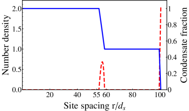
Figure 1: (Color online) Number density profile (solid line; scale on left axis of graph) and condensate fraction (dashed line; scale on right axis of graph) of an inhomogeneous lattice boson system. From inner to outer of the system, the phases (thickness in lattice spacing $d_{s}$) are the Mott-insulator (55), condensate (5), the Mott-insulator (38), and condensate (2).

II.3 Inhomogeneous system

For inhomogeneous lattices, local condensate order can be studied by replacing the chemical potential $\mu$ with $(\mu-V_{i})$, corresponding to the local density approximation. Because of the spatial variance of $V_{i}$, the system is expected to display Mott-insulator phases and condensate phases that are spatially separated Fisher89 ; Jaksch98 . In a three-dimensional (3D) deep lattice, for example, if the potential is a radially symmetric harmonic trap ($V_{i}=m\omega^{2}_{t}r_{i}^{2}/2$), the system will have a concentric shell structure with thick Mott-insulator shells alternating with thin condensate shells. The density profile of this system resembles the side view of a wedding cake (Fig. 1).

In Fig. 1, we plot the profile for an experimentally feasible system containing $N=5.11\times 10^{6}~{}^{87}$Rb atoms with $a_{s}=5.32$ nm in a sphere whose radius is $53.2~{}\mu$m, or 100 sites, long. The parameters of the optical lattice are $\lambda=1.064~{}\mu$m and $V_{0}=20E_{R}$ and the frequency of the external harmonic trap is $\omega_{t}=2\pi\times 6.13$ Hz. The system has an $n=2$ Mott-insulating sphere, an $n=1$ Mott-insulating shell, a condensate shell between the two Mott-insulators, and a condensate shell on the outer boundary. The thickness of the condensate interlayer is $2.66\mu$m or 5 sites long, approximately ten times thinner than the Mott-insulating regime. We use this setting to simulate the rf spectroscopy experiment in Sec. III.

III rf spectroscopy

One effective probe of the structure of lattice bosons is the high-resolution microwave spectroscopy. In recent experiments, an external rf is applied to induce ⁸⁷Rb atoms to make hyperfine transitions from $\left|F=1,m_{F}=-1\right\rangle$ state to $\left|F=2,m_{F}=1\right\rangle$ state Matthews98 ; Campbell06 or to $\left|F=2,m_{F}=0\right\rangle$ state Folling06 . In this section, we propose variants of the experiment of Ref. Campbell06 in which the Mott-insulating shells with different occupation numbers have been resolved by analyzing the density-dependent clock shifts of the system. The resolution hinges on the energy differences of interaction among two atoms in the same hyperfine state versus in different hyperfine states.

In order to probe the condensate in the deep-lattice regime, we propose specific values of lattice parameters that would distinguish the spectrum of the Mott-insulator state and that of the condensate state in two ways. The first is that the former would have one resonant peak, but the latter would have two. The second is that the two peaks of the latter would be blue-shifted with respect to that of the former. The scales for the separation between the two peaks and the shift are of a order of a few Hz, and we anticipate that they will be within experimental reach in the near future, providing an effective means to verify the existence of the condensed interlayers. By considering the effect of Goldstone modes and finite-temperature, we show that this signal is a signature of condensate order, and would be absent if the interlayers were a normal boson fluid of the same density.

Below, we begin with a discussion of our rf setup applied to a homogeneous system and then use these results to derive the spectrum of the inhomogeneous system in the local-density approximation. We use numerical simulations where appropriate and also invoke Fermi’s golden rule to analyze the rf spectra for a range of phase space. To summarize our findings: at zero-temperature, the Mott-insulator and condensate states can be clearly distinguished via their single-peak versus double-peak structures. For the set of proposed parameters, rf transitions into states containing Goldstone mode excitations (which are the low-energy excitations associate with the condensate) do not obscure the double-peak structure at zero temperature. However, at finite temperature, thermal excitations affect the two-peak structure. At very low temperatures ($k_{B}T\ll ZJ$), Goldstone modes lead to a temperature-dependent broadening of the peaks in the condensate signal. At higher temperatures ($k_{B}T\sim ZJ\ll U$), thermal fluctuations destroy the condensate order to yield a normal fluid; $k_{B}T_{c}$ is of order $ZJ$ Barankov07 ; Gerbier07 . In this temperature regime, Goldstone modes completely obliterate the peaks, and extra structure develops at other characteristic frequencies corresponding to new allowed hyperfine transitions. At temperatures $k_{B}T>U$, the system displays large density fluctuations, even in the regions that are Mott-insulating at zero temperature, and the system loses signs of its quantum phases. Our analysis is thus limited to temperatures much less than the interparticle interaction, $U\sim k_{B}\times 10$ nK wherein, as a function of temperature, the resolution of the peaks in the rf spectrum tracks the condensate order and its ultimate destruction at $T_{c}$.

III.1 Zero-temperature rf spectrum: Decoupled-sites

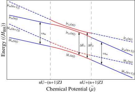
Figure 2: (Color online) Energies of the lowest four single-site states of the 2-species Bose-Hubbard Hamiltonian. The corresponding states, which are defined in Eqs. (7-11), are marked for each curve. In the mid-region (marked red), the ground state of the system is a condensate, while on the sides (marked blue), it is a Mott-insulator.In each region, the ground state can make transitions to those higher energy states denoted with solid lines (with corresponding energy gaps marked by the black arrows), but is forbidden from transitions to those states marked with dashed lines.

For a uniform system of two-state ($|a\rangle$ and $|b\rangle$) bosons, the Bose-Hubbard Hamiltonian contains two tunneling strengths ($J_{a}$ and $J_{b}$), three interaction strengths ($U_{a}$, $U_{b}$, and $U_{ab}$), the chemical potential, and the single-particle energy difference between $a$ and $b$ particles ($\omega_{ba}$). In the following, we consider a particular case: $J_{b}=0$, $U_{b}\gg U_{a}$, $U_{ab}=U_{a}$, and $\omega_{ba}\gg U_{a}$. This setting has two advantages. (1) Because $\omega_{ba}>0$, the ground state of the system has all particles in the $a$ hyperfine state but no particles in the $b$ state. (2) Because $U_{b}\gg U_{ab}=U_{a}$, the energy gap between having two $b$ particles on a site and having one $b$ particle is much larger than that between having one $b$ particle on a site and having no $b$ particles. Therefore when the frequency of the rf field is of the order of the gap in the latter case, we can safely limit consideration to transitions to states with one $b$ particle.

For the situation described above, the Bose-Hubbard Hamiltonian, including the upper hyperfine state, becomes

$$-J\sum_{<ij>}(\hat{a}_{i}^{\dagger}\hat{a}_{j}+\hat{a}_{j}^{\dagger}\hat{a}_{i})+\sum_{i}[\frac{U}{2}(\hat{n}_{ai}+\hat{n}_{bi})(\hat{n}_{ai}+\hat{n}_{bi}-1)$$

$$-{\mu}(\hat{n}_{ai}+\hat{n}_{bi})+\frac{U_{b}-U}{2}\hat{n}_{bi}(\hat{n}_{bi}-1)+\omega_{ba}\hat{n}_{bi}],$$ (6)

where we drop the subscript $a$ of $J_{a}$ and $U_{a}$. In the deep lattice regime, we use the mean-field approximation to analyze the rf spectrum of the system. The single-site Mott-insulator state with $\left\langle{\hat{n}}\right\rangle=n$ and the single-site condensate state with $n<\left\langle{\hat{n}}\right\rangle<n+1$ can be represented by

$$\left|{\psi_{m}(n)}\right\rangle = \left|n\right\rangle\otimes\left|0\right\rangle,$$

$$\left|{\psi_{c}(n)}\right\rangle = \sin\frac{\theta}{2}\left|n\right\rangle\otimes\left|0\right\rangle+\cos\frac{\theta}{2}\left|{n+1}\right\rangle\otimes\left|0\right\rangle,$$ (7)

where $\left|{n_{a}}\right\rangle\otimes\left|{n_{b}}\right\rangle$ represents a single-site state with $n_{a}$ particles of hyperfine state $a$ and $n_{b}$ particles of hyperfine state $b$. As in Eq.(9) of Sec. II.2, we have $\cos\theta=(\mu-nU)/[(n+1)ZJ]$ determining the angle between the pseudo-spin and the $z$ axis. Compared to Eq.(9), the symmetry-breaking phase $\phi$ has been set to zero for the decoupled-site analysis; the subsequent Goldstone mode analysis implicitly assumes that this phase has gradual variations from site to site.

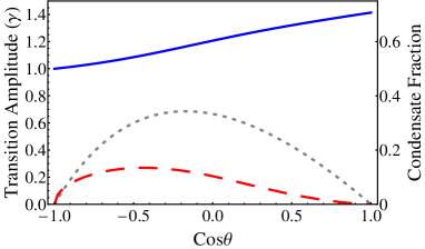
Figure 3: (Color online) Absolute value of transition amplitude $A_{1t}$ and $A_{2t}$ (solid and dashed lines, respectively; axis on left-hand side of graph) and condensate fraction (dotted line; axis on right-hand side of graph) as a function of the value of the cosine of the pseudo-spin angle (corresponding to the density of bosons). The system is a uniform condensate whose number density satisfies $1<{\left\langle n\right\rangle}<2$.

The Hamiltonian describing the interaction between the bosons and an applied rf field is DeMarco05

$${\cal H}_{rf}=\sum_{i}\gamma(\hat{a}_{i}^{\dagger}\hat{b}_{i}+\hat{b}_{i}^{\dagger}\hat{a}_{i})\cos\omega t,$$ (8)

where $\gamma$ is proportional to the amplitude of the rf field and $\omega$ is its frequency; this Hamiltonian can be derived from the second-quantized form of the interaction $\int{d}\mathbf{r}\psi^{\dagger}\hat{\mathbf{\mu}}\cdot\mathbf{B}\psi$.

We analyze the allowed transitions in different ranges of the chemical potential. We evaluate the transition amplitudes $A_{t}=\left\langle F\right|\sum_{i}\gamma(\hat{a}_{i}^{\dagger}\hat{b}_{i}+\hat{b}_{i}^{\dagger}\hat{a}_{i})\left|I\right\rangle$ between allowed initial and final states $\left|I\right\rangle$ and $\left|F\right\rangle$, respectively, and the energy gaps $\Delta E$, given by the difference in the expectation values of the Bose-Hubbard Hamiltonian of Eq. (6) in the corresponding excited state and ground state. We plot the energy levels in Fig. 2, which shows how the system at zero temperature undergoes quantum phase transitions through the $n$ Mott-insulator state [$|{\psi_{m}(n)}\rangle$], the condensed state [$|{\psi_{c}(n)}\rangle$], and the $n+1$ Mott state [$|{\psi_{m}(n+1)}\rangle$] as the chemical potential is increased. The figure also shows possible excited states to which the ground state can make a transition in the presence of the rf field and shows the energy gap between them. Details of the transitions for each range of the chemical potential in Fig. 2 are discussed below.

When $[(n-1)U+nZJ]<\mu<[nU-(n+1)ZJ]$, the ground state is the $n$ Mott-insulator state $[\left|{\psi_{m}(n)}\right\rangle]$. We have only one possible excited state [denoted by $\left|e_{m}(n)\right\rangle$] to which the ground state can make a transition. The excited state, the transition amplitude $A_{t}$, and the energy gap $\Delta E$ are correspondingly

$$\left|e_{m}(n)\right\rangle=\left|{n-1}\right\rangle\otimes\left|1\right\rangle,{\textrm{ }}A_{t}=\gamma\sqrt{n},{\textrm{ }}\Delta E=\omega_{ba}.$$ (9)

Because $\Delta E$ is independent of $n$, all the Mott-insulator states with different $n$ have the same energy gap between the ground state and the excited state.

When $[nU-(n+1)ZJ]<\mu<[nU+(n+1)ZJ]$, the ground state is the condensate state $\left|{\psi_{c}(n)}\right\rangle$. We find two orthogonal excited states [denoted by $\left|{e_{c1}(n)}\right\rangle$ and $\left|{e_{c2}(n)}\right\rangle$] with nonzero transition amplitudes. The first state, its corresponding transition amplitude $A_{t1}$, and energy gap $\Delta E_{1}$ are

$$\left|{e_{c1}(n)}\right\rangle = \sin\frac{{\theta_{1}}}{2}\left|{n-1}\right\rangle\otimes\left|1\right\rangle+\cos\frac{{\theta_{1}}}{2}\left|n\right\rangle\otimes\left|1\right\rangle,$$

$$A_{1t} = \gamma(\sqrt{n}\sin\frac{\theta}{2}\sin\frac{{\theta_{1}}}{2}+\sqrt{n+1}\cos\frac{\theta}{2}\cos\frac{{\theta_{1}}}{2}),$$

$$\Delta E_{1} = \omega_{ba}+\frac{{ZJ\sqrt{n+1}}}{4}[\sqrt{n+1}(\sin^{2}\theta+2)$$ (10)

$$- (\sqrt{n}\sin\theta\sin\theta_{1}+2\sqrt{n+1}\cos\theta\cos\theta_{1})],$$

where $\left|e_{c1}\right\rangle$ is taken to be the equilibrium state (the lowest energy state) of the Hamiltonian with the constraint $n_{b}=1$ (i.e., in the $n_{b}=1$ block). We calculate the parameter $\theta_{1}$ by minimizing the energy of the system with site $i$ in an excited state [$\left|{e_{c1}(n)}\right\rangle$] and all the other sites still in the ground state [$\left|{\psi_{c}(n)}\right\rangle$]. As a result, we obtain a relation between $\theta_{1}$ and $\theta$, which is $\tan\theta_{1}=\sqrt{n/(n+1)}\tan\theta$. The second excited state, corresponding transition amplitude $A_{t2}$, and energy gap $\Delta E_{2}$ are

$$\left|{e_{c2}(n)}\right\rangle = \cos\frac{{\theta_{1}}}{2}\left|{n-1}\right\rangle\otimes\left|1\right\rangle-\sin\frac{{\theta_{1}}}{2}\left|n\right\rangle\otimes\left|1\right\rangle,$$

$$A_{2t} = \gamma(\sqrt{n}\sin\frac{\theta}{2}\cos\frac{{\theta_{1}}}{2}-\sqrt{n+1}\cos\frac{\theta}{2}\sin\frac{{\theta_{1}}}{2}),$$

$$\Delta E_{2} = \omega_{ba}+\frac{{ZJ\sqrt{n+1}}}{4}[\sqrt{n+1}(\sin^{2}\theta+2)$$ (11)

$$+ (\sqrt{n}\sin\theta\sin\theta_{1}+2\sqrt{n+1}\cos\theta\cos\theta_{1})].$$

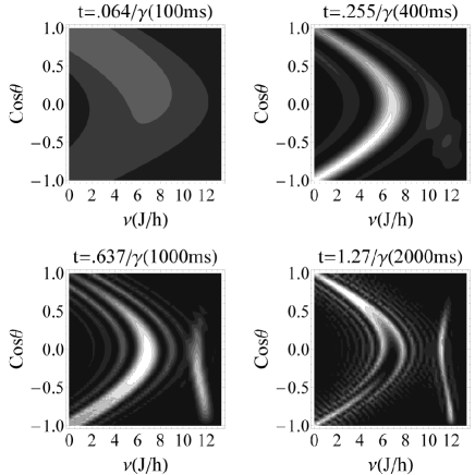
Figure 4: Fraction of bosons transferred to the higher hyperfine state for a uniform condensate with $1<{\left\langle n\right\rangle}<2$ at $t=100$, 400, 1000, and 2000 ms. The horizontal axis is the detuning of the rf field with respect to the resonant frequency of the Mott-insulating state, while the vertical axis is $\cos\theta$. The color scale is bounded by 0 (black) and 1 (white) with contours separated by 0.1.

When the chemical potential in the condensed phase reaches its upper or lower bound ($\theta=0$ or $\theta=\pi$), Eq. (10) becomes Eq. (9) with $n$ or $n+1$ Mott-insulator states correspondingly, but the transition amplitude of Eq. (11) vanishes (Fig. 3). However, the $n=0$ condensate state is an exception since it can only make a transition to one excited state $\left|{0}\right\rangle\otimes\left|1\right\rangle$ with a transition amplitude $\gamma\cos{\frac{\theta}{2}}$ and an energy gap $(\omega_{ba}+JZ\sin^{4}\frac{\theta}{2})$.

Thus, while the Mott state can only make a transition to one excited state, the condensate state can make transitions to two excited states.

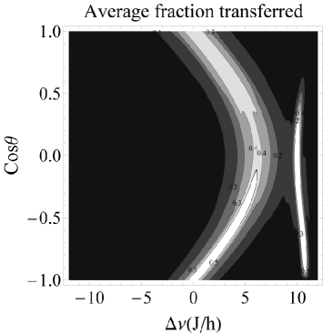
Figure 5: Average fraction of bosons transferred between $t=1000$ and $2000$ ms. Contour interval is $0.1$. The first peak appears in the range of $0$ to $7J$ ($6.29$ Hz), and the second peak appears at about $11.5J$ ($10.3$ Hz). When $\cos\theta=\pm 1$, we recover the Mott signature.

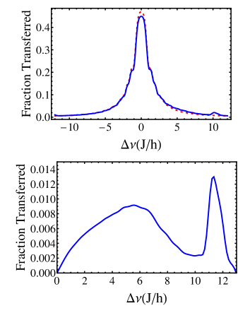
Figure 6: (Color online) Average fraction of bosons transferred between $t=1000$ ms and $2000$ ms for the inhomogeneous system defined in Fig. 1. Up: the system with both Mott-insulator and condensate regions (solid) compared with that having only Mott-insulator regions (dotted). Down: spectrum of the condensate shells after eliminating the contribution from the Mott -insulator shells. The results show that two peaks with positive shifts are signatures of condensate order in a deep optical lattice.

As a consequence of these allowed transitions, the Mott-insulator state ought to have a single peak in the associated rf spectrum while the condensate ought to have two. This can be seen to first order (in number of particles transferred) by employing Fermi’s golden rule (FGR), where the transition rate is given by  Pethick01

$$I(\omega)=\frac{2\pi}{\hbar}\sum_{F,I}{(\rho_{I}-\rho_{F})\left|{A_{t}}\right|^{2}}\delta\left({\omega-E_{F}+E_{I}}\right),$$ (12)

where $\left|I\right\rangle$ ($\left|F\right\rangle$) is the initial (final) state with energy $E_{I}$ ($E_{F}$) and probability for occurrence $\rho_{I}$ ($\rho_{F}$). Hence, FGR would predict a single delta function peak for the Mott-insulator state rf spectrum and two delta function peaks for the condensate.

We now confirm that the presence of the condensate does yield a two-peak rf spectrum by numerically time evolving the equations of motion in the presence of the rf field. Taking into account both experimental feasibility and optimal conditions for observing the rf signatures of the condensate, we consider the setting of Fig. 1. This setting corresponds to the values $U=2\pi\times 306$ Hz, $J=2\pi\times 0.898$ Hz (then $ZJ/U=1.76\times 10^{-2}$ is small compared to $1$), and $\mu=1.5U$. The intensity of the rf field is set such that $\gamma=0.118ZJ=2\pi\times 0.637$ Hz, which is of the same order as that in the experiment of Ref. Campbell06 . If the rf field is turned on at $t=0$, within the rotating-wave approximation we find that the fraction of transferred particles at the frequency of the second peak of the condensate’s spectrum begins to rise at $t=0.225/\gamma$ ($400$ ms), and that at any given time, the spectrum shows oscillatory behavior with respect to the detuning (Fig. 4). In order to see a distinct second peak, we calculate the average fraction transferred between $t=0.637/\gamma$ ($1000$ ms) and $t=1.27/\gamma$ ($2000$ ms). Figure 5 shows the average fraction transferred for a uniform condensate. We can see two peaks whose positions agree with the energy gap in Eqs. (10) and (11). Figure  6 shows the average fraction transferred for the entire inhomogeneous system. Because the fraction transferred in the Mott-insulator is an even function of the detuning, we subtract the negative detuning part from the corresponding positive detuning part to eliminate the contribution of the Mott-insulator. The result shows that there are two peaks of magnitude 1% ($5\times 10^{5}$ atoms transferred), and their positions agree with our theoretical analysis.

All calculations above rely on a mean-field approximation. As a minor check that number conservation and entanglement do not alter the proposed signatures, we performed the numerical toy simulation os time-evolving the entangled, fixed-number condensate state of six bosons in four sites in the presence of an rf field (Appendix C). Even such small system sizes has been shown to exhibit salient features of the superfluid-Mott-insulator phase transition in macroscopic systems Luhmann08 . The results show the same signatures as those of the mean-field approach: two peaks with positive shifts of order $J$, thus providing some confidence that our result is not an artifact of the mean-field approximation.

To ensure that no spurious effects emerge from truncating the Hilbert space, we have analyzed the effect of the leading subdominant states $\left|{n-1}\right\rangle\otimes\left|0\right\rangle$ and $\left|{n+2}\right\rangle\otimes\left|0\right\rangle$. Within the resultant four-state truncated space, we obtain four possible final states. Two of them have the same energy shifts (of order $J$) and transition amplitudes (of order $\gamma$) as those obtained in the two-state truncated space, plus small corrections of order $J/U$; these corrections contribute a fraction $(J/U)^{2}$ to the number transferred. The other two final states have energy shifts of order $U$ ($\gg J$) and transition amplitudes of order $\gamma J/U$ ($\ll\gamma$), which also contributes a fraction $(J/U)^{2}$ to the number transferred. The minimal change coming from taking into account these additional states justifies our usage of the two-state truncation in the deep lattice regime.

III.2 Goldstone modes and finite-temperature effects

At finite temperature, the thermally-occupied excited states of the system will affect the rf spectrum. When the temperature is much smaller than the interaction energy ($k_{B}T\ll U$), the Mott-insulator state has negligible thermal effects because it has an excitation gap of order $U$ DeMarco05 ; Pupillo06b ; Konabe06 . However, we should be concerned that the two-peak signature of the condensate may be destroyed at low temperatures by Goldstone modes associated with the continuous symmetry-breaking in the phase $\phi$ of the condensate ground-state wave function. Each Goldstone mode or boson corresponds to a long-wavelength distortion of the density and phase between neighboring sites and the modes form the gapless low-energy excitation spectrum for the condensate. The structure of these modes has been derived from the pseudo-spin formulation and analyzed for homogeneous and inhomogeneous systems in Ref. Barankov07 . In order to be self-contained, we present the Goldstone-mode description here in Appendix B for the homogeneous generalized case of the two-species system of interest in this paper.

At zero temperature, the initial state consists of the ground state of the system purely comprised of $a$ particles, and thus no Goldstone modes are excited. Under an rf field however, a small number of particles change their internal state to $b$. If this change is not uniform in space, it will be accompanied by Goldstone modes. Assuming that $N_{G}$ is the total number of Goldstone bosons excited by the rf field, we can estimate the final-state energy of a single site, which differs from that of the $N_{G}=0$ case, as $(N_{G}/M)ZJ$, where $M$ is the total number of sites and $ZJ$ is the energy scale of the Goldstone-mode spectrum. If the rf field is weak enough that the average number of excited Goldstone bosons per site ($N_{G}/M$) is much smaller than one, the change in the single-site energy gap is much smaller than $ZJ$, which is about the distance between the two peaks obtained in the Sec. II. In typical experimental settings, this indeed is the case given that about $10\%$ of the particles make transitions to the $b$ state. Therefore, exciting Goldstone modes at zero temperature ought not obscure the two-peak signature; in Appendix B, we explicitly show that these modes provide a small background which still leaves the two-peak signature robust.

At finite temperature, in three dimensions, the condensate density is reduced by the existence of thermally excited Goldstone modes. As argued in Appendix B, for low temperatures $kT\ll ZJ$, we expect a slight reduction in the height of the two peaks and a slightly larger contribution to the background. Nevertheless, for three-dimensional systems, we expect the two-peak condensate signature to persist at these temperatures.

Close to the critical temperature $kT_{c}\approx ZJ$ (see Ref.  Barankov07 ; Gerbier07 ), we expect the average thermal expectation value $\sum{{}_{j}}\langle{a_{j}}\rangle/N$ of the order parameter to vanish, corresponding to destruction of long-range order in the system. Within the decoupled-site mean-field approximation, $\langle{a_{i}}\rangle$ fluctuates in magnitude and phase from site to site. The kinetic part of the mean-field energy in the Bose-Hubbard Hamiltonian can thus be thought of as having a spread of order $(n+1)ZJ$. Given that the two low-temperature peaks in the rf spectrum are also separated by about $(n+1)ZJ$, we predict that the two peaks merge into a continuum around the critical temperature. In two-dimensions, even the smallest temperature suffices for the Goldstone modes to destroy true long-range order and we believe that this will be reflected in the smearing out of the two-peak structure for low-dimensional systems.

Finally, for the inhomogeneous shell situation, the Goldstone modes become quantized due to confinement Barankov07 . Reference Barankov07 provides a discussion of the mode structure and dimensional crossover as a function of temperature. The essential issue is whether the quantized modes along each direction which are accessible at temperature $T$ are numerous enough to form an effective continuum. Modifying the arguments above to include these inhomogeneous effects, we deduce that the two peak structure would remain at low temperatures for a condensate shell with a thickness of several lattice sites.

In summary, our arguments indicate that the presence of condensate order can be detected in a two-peak rf spectrum for appropriate rf parameter settings in contrast to the one-peak structure of the Mott-insulator phase. Our results also suggest that when the condensate becomes a normal fluid at $T=T_{c}$, the two-peak structure is washed out. Our arguments can be made more rigorous by way of numerical simulations such as those of Sec. IIIA that would include the Goldstone modes and finite temperature effects; such a treatment is beyond the scope of this paper.

IV Matter wave interference

Experimental observation of matter-wave interference peaks in absorption images have provided striking evidence for superfluid states in shallow optical lattices Greiner02 . In addition, the concentric Mott-insulating-shell system has been observed to preserve finite visibility in the interference pattern Gerbier05a ; Gerbier05b . Characteristics of the interference patterns have been analytically and numerically studied under several specific conditions for normal fluid, superfluid and Mott-insulating phases in the lattice boson system Roth03 ; Diener07 ; Lin08 ; Toth08 . Here, we consider bosons in the deep lattice regime and ask what signatures of matter-wave interference can distinguish the presence of a condensate shell between two Mott-insulating shells. We work at zero temperature, which should be valid for temperatures $kT\ll J$, where one would expect the contrast between these states to be strongest. We begin by considering a homogeneous system, where the many-body wave functions of the Mott-insulating and deep-lattice condensate phases can be exactly time-evolved to obtain the density profile measured by absorption imaging. For simplicity, we ignore the effect of interaction during time of flight Roth03 , which is expected to quantitatively influence the intensity and width of peaks but preserve the qualitative signatures of the interference pattern Lin08 . By calculating the time-evolution of a system of bosons on a ring lattice, we show that condensate states will have sharp interference maxima, in contrast to Mott-insulator states, after free expansion of the system. To illustrate how these features would be displayed in an inhomogeneous system, we also the time evolution of a system of concentric ring lattices that have a Mott-condensate-Mott structure and point to signatures of the condensate in the time-evolved profiles.

IV.1 Density profile upon expansion for homogeneous systems

For the Mott-insulator state $\left|{\left|n\right\rangle}\right\rangle$, the many-body wave function is a product of $N$ single-particle wave functions:

$$\Psi({\bf{r}}_{1},\ldots,{\bf{r}}_{N}) \equiv \left\langle{{{\bf{r}}_{1},\ldots,{\bf{r}}_{N}}}\mathrel{\left|{\vphantom{{{\bf{r}}_{1},\ldots,{\bf{r}}_{N}}{\left|n\right\rangle}}}\right.\kern-1.2pt}{{\left|n\right\rangle}}\right\rangle$$ (13)

$$= A\sum_{\textrm{sym}\{{\bf{r}}\}}{\prod_{i=1}^{N}{\psi({\bf{r}}_{i}-{\bf{s}}^{(i)})}}$$

$$= A\sum_{\{{\bf{s}}\}}{\prod_{i=1}^{N}{\psi({\bf{r}}_{i}-{\bf{s}}^{(i)})}},$$

where ${\psi({\bf{r}}_{i}-{\bf{s}}^{(i)})}$ is the single particle wave function of particle $i$ localized on a site at position ${\bf{s}}^{(i)}$, and $A$ is a normalization constant. To satisfy Bose-Einstein statistics, we need to symmetrize all $N$ degrees of freedom; this symmetrization (denoted by $\sum{{}_{\textrm{sym}\{{\bf{r}}\}}}$) is equivalent to the sum over all configurations of $\{{\bf{s}}^{(i)}\}$ (denoted by $\sum{{}_{\{{\bf{s}}\}}}$), which are permutations of $\{{\underbrace{{\bf{s}}_{1},\ldots,{\bf{s}}_{1}}_{n},\underbrace{{\bf{s}}_{2},\ldots,{\bf{s}}_{2}}_{n},\ldots\underbrace{{\bf{s}}_{M},\ldots,{\bf{s}}_{M}}_{n}}\}$, where ${{\bf{s}}_{j}}$ is the position of site $j$.

Near the center of a lattice site, the lattice potential can be approximated as harmonic with frequency $\omega=\sqrt{4{V_{0}}{E_{R}}}/\hbar$, where $V_{0}$ is the depth of the optical lattice and $E_{R}$ is the recoil energy. The single-particle wave function can thus be approximated as a harmonic oscillator ground-state wave function well-localized on a site. If we ignore interactions (valid at low density), after turning off the lattice potential and the trap potential all single-particle wave functions are time-evolved by the free particle Hamiltonian ${\bf{\hat{p}}}^{2}/2m$. The wave function at later times is then given by

$$\psi_{t}({\bf{r}}_{i}-{\bf{s}}^{(i)})=\left({\frac{{2l^{2}}}{\pi}}\right)^{d/4}\frac{{\exp[-({\bf{r}}_{i}-{\bf{s}}^{(i)})^{2}/(l^{2}+2i\hbar t/m)]}}{{(l^{2}+2i\hbar t/m)^{d/2}}},$$

where $d$ is the dimensionality of the system, and $l$ is the characteristic length of the single-particle wave function Griffiths05 ; Toth08 . The density profile as a function of position and time is obtained by calculating the diagonal elements of the single-particle density matrix Leggett06 ;

$$\rho(r,t) \equiv N\int{\Psi_{t}^{*}({\bf{r}},{\bf{r}}_{2},\ldots,{\bf{r}}_{N})\Psi_{t}({\bf{r}},{\bf{r}}_{2},\ldots,{\bf{r}}_{N})d{\bf{r}}_{2}\ldots d{\bf{r}}_{N}}$$ (15)

$$= N\left|A\right|^{2}\sum_{\{{\bf{s}}\}}{\sum_{\{{\bf{s^{\prime}}}\}}{\psi_{t}^{*}({\bf{r}}-{\bf{s}}^{(1)})\psi_{t}({\bf{r}}-{\bf{s^{\prime}}}^{(1)})}}$$

$$\times\exp[-\sum_{i=2}^{N}{({\bf{s}}^{(i)}-{\bf{s^{\prime}}}^{(i)})^{2}/(2l^{2})}].$$

For the condensate state $\left|\Psi\right\rangle$ of Eq. (2), the density profile is given by

$$\rho_{c}(r,t) = N\left|{A}\right|^{2}\sum_{\{\eta\}}{\sum_{\{\eta^{\prime}\}}{C_{\{\eta^{\prime}\}}^{*}C_{\{\eta\}}}}$$ (16)

$$\times \{{\sum_{\{{\bf{s}};\{\eta\}\}}{\sum_{\{{\bf{s^{\prime}}};\{\eta^{\prime}\}\}}{\psi_{t}^{*}({\bf{r}}-{\bf{s}}^{(1)})\psi_{t}({\bf{r}}-{\bf{s^{\prime}}}^{(1)})}}}$$

$$\times \exp[-\sum_{i=2}^{N}{({\bf{s}}^{(i)}-{\bf{s^{\prime}}}^{(i)})^{2}/(2l^{2})}]\},$$

where $\sum{{}_{\{\eta\}}}$ denotes the same sum in Eq. (2), and $\sum{{}_{\{\bf{s};\{\eta\}\}}}$ denotes the sum over all $\{{\bf{s}}^{(i)}\}$ with a specific ${\{\eta\}}$; $\{{\bf{s}}^{(i)}\}$ are permutations of the set including $n+1$ each ${\bf{s}}_{\eta_{i}}$ of the sites $\eta_{1},\ldots,\eta_{M_{1}}$ and $n$ each ${\bf{s}}_{j}$ of the other sites. If $M_{1}=0$ or $M_{1}=M$, ${\{\eta\}}$ has only one configuration, and hence Eq. (16) becomes Eq. (15).

IV.2 Example: Expansion of bosons in a ring lattice

As a concrete case that shows how sharp interference peaks emerge upon release and expansion of the condensate, we consider the illustrative example of bosons in a one-dimensional lattice of sites located on a ring of radius $s$ in a two dimensional plane. Because of the symmetry of the ring, constructive interference is expected at its center. We therefore calculate the center density contributed by one particle, defined as $\tilde{\rho}(t)\equiv\rho(0,t)/N$. The result is

$$\tilde{\rho}(t)=F\left({\frac{{2l^{2}}}{\pi}}\right)^{d/2}\frac{{\exp[-2s^{2}l^{2}/(l^{4}+4\hbar^{2}t^{2}/m^{2})]}}{{(l^{4}+4\hbar^{2}t^{2}/m^{2})^{d/2}}},$$ (17)

where $d=2$ for this system and $F$ is equal to

$$F_{M}=\left|A\right|^{2}\sum_{\{{\bf{s}}\}}{\sum_{\{{\bf{s^{\prime}}}\}}{\exp[-\sum_{i=2}^{N}{({\bf{s}}^{(i)}-{\bf{s^{\prime}}}^{(i)})^{2}/(2l^{2})}}}]$$

for the Mott-insulator state and

$$F_{c} = \left|A\right|^{2}\sum_{\{\eta\}}{\sum_{\{\eta^{\prime}\}}{C_{\{\eta^{\prime}\}}^{*}C_{\{\eta\}}}}$$

$$\times\{\sum_{\{{\bf{s}};\{\eta\}\}}{\sum_{\{{\bf{s^{\prime}}};\{\eta^{\prime}\}\}}{\exp[-\sum_{i=2}^{N}{({\bf{s}}^{(i)}-{\bf{s^{\prime}}}^{(i)})^{2}/(2l^{2})}]}}\}$$

for the condensate. If $s\gg l$, $\tilde{\rho}(t)$ has a maximum at

$$t_{m}=mls/\sqrt{d}\hbar$$ (18)

and a half width $\Delta{t}=2^{1/d}mls/\hbar$. While $t_{m}$ indicates the time it takes matter waves to disperse from the ring to the center, $\Delta{t}$ measures the duration of constructive interference processes. Equation (18) is of the same form as a continuum superfluid confined to a shell geometry with the characteristic length $l$ given by the thickness of the shell Lannert07 . The terms with $\{\eta^{\prime}\}=\{\eta\}$ in the sum for $F$ are the same for the Mott-insulator and condensate states. However, $F$ for the condensate state has many additional terms with $\{\eta^{\prime}\}\neq\{\eta\}$ that contribute to the center density which are not present in $F_{M}$. Therefore, we see that the center density of the condensate state has a much sharper peak than that of the Mott-insulator state. At finite temperature, the interference pattern is the thermal average over the densities of all possible pure states. The coefficients $C_{\{\eta\}}$ of higher energy states are not necessarily real and positive and thus would decrease the value of $F$ given that not all terms give positive contributions. Therefore, we expect that the interference pattern of a condensate becomes more blurred with increasing temperature.

Although here we have only analytically solved for the density at the center of the ring, constructive interference patterns will occur throughout space after the system is released from its ring trap. The differences in these spatial patterns between initial Mott-insulator and initial condensed states gives further evidence for condensate order. As a toy example that exhibits these patterns, we numerically simulated the expansion processes of a four-site Mott-insulator and a four-site condensate in the ring geometry (Appendix C). Although the initial density profiles of the two cases look the same, their interference patterns behave quite differently during the expansion process.

IV.3 Inhomogeneous systems

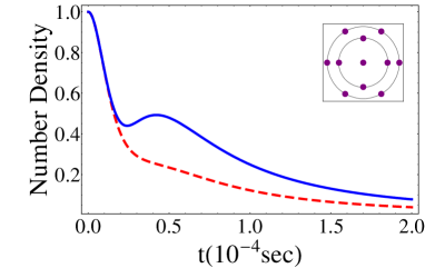
Figure 7: (Color online) Density at the center point, as a function of time, during expansion of the system. The inset shows the geometry and the site positions of the model. The solid curve corresponds to the system that has a center site and an outer ring in Mott-insulating states and the inner ring in the condensate state. The dashed curve corresponds to the control system with the inner ring in the Mott-insulating state. The vertical axis is the relative density with respect to the initial value. The peak and the relatively large value at long times are evidence of the condensate part of the system.

The above discussions show how homogeneous systems of condensate and Mott-insulator display different patterns upon release and expansion and that interference is a signature of condensate order in the system. To illustrate how these signatures can be used to probe condensate order realistic experimental situations, we consider a simplified inhomogeneous system of ⁸⁷Rb atoms displaying the nested, or “wedding-cake,” structure of bosons in optical lattices in the presence of a harmonic trap. Building on the results of the previous section for bosons on a ring lattice, we model a two-dimensional system made up of a center point and two concentric rings, where the central site is in the $n=2$ Mott-insulating state, the four sites in the inner ring are in the ${\left\langle n\right\rangle=1.5}$ condensate state, and six sites in the outer ring are in the $n=1$ Mott-insulating state. Site spacings of the two rings are both $d_{s}=0.532~{}\mu$m. For the lattice depth $V_{0}=20E_{R}$, the characteristic length of the initial single-particle wave function is $l=0.283d_{s}$. If the lattice potential is turned off at $t=0$, the density at the center point as a function of time shows a peak at $t=4.2\times 10^{-5}$ s (Fig. 7). Compared to a control system where the inner ring has Mott-insulator states of the same density ($2$ sites in $n=2$ and $2$ sites in $n=1$), the peak and the larger long-time residual density in the center indicate large constructive interference due to the condensate part of the system. Considering expansion of a 3D inhomogeneous system of Fig. 1, we expect to observe a density peak in the center of the sphere at $t=3.67$ ms, which is about $1/4$ the duration of the time of flight in the experiment of Ref. Greiner02 . We expect that such a time-evolved density profile should also be able to discern the presence of condensate interlayers for larger systems with realistic numbers of bosons.

In summary, we obtain interference signatures of a thin condensate inter-layer between two Mott-insulator layers. For a toy system exhibiting concentric co-existent phases, we show that the condensed phase contributes a sharp peak to the time-evolved central particle density. As performed for single phases, simulations of realistic inhomogeneous large-sized three-dimensional systems within our truncated wave function basis and extraction of measurable quantities, such as the visibility, are in order; we believe that our results here are indicative of the signatures of the condensate layer that would be obtained in actual systems.

V Summary

Systems of atoms in optical lattices provide a seemingly-ideal system for exploring the quantum phases of bosons. Generically, experimentally-studied systems are not of uniform density, due to the confining trap. This leads to the coexistence of Mott-insulating and condensate phases within a single system at fixed lattice depth and complicates the study of these phases. Here, we have considered bosons in deep optical lattices, where condensate phases exist between Mott-insulator phases, but are close to their quantum transition to the Mott-insulator phase. We have justified the use of a mean-field approximation by constructing the entangled, fixed-number, many-body wave function and showing that many key aspects of this phase (in particular, the condensate fraction and the on-site number fluctuations) are identical in the two descriptions. Toward developing experimental tests of the condensate interlayers in inhomogeneous systems, we have calculated the condensate signal using two common probes of cold-atom systems: rf spectroscopy and release-and-expansion. We have shown specific features of the signal in these probes that distinguish the condensate regions from the Mott phases. We have shown that the rf signal specifically probes condensate order in that these characteristic features disappear when the condensate is replaced by a normal fluid as a result of thermal fluctuations. We hope that our work will enable closer exploration of the structure of coexisting Mott-insulator-condensate phases in realistic experimental situations.

VI Acknowledgements

We are grateful to B. DeMarco, K. R. A. Hazzard, A. J. Leggett, E. J. Mueller, and M.-H. Yung for involved discussions and G. Baym for his perceptive remarks. We would like to thank R. Barankov for his input during the initial stages of this work and for his insights into the Goldstone-mode structure in the case of a single species of bosons. C.L. and S.V. would like to acknowledge the gracious hospitality of the Aspen Center for Physics where some key aspects of this research were sorted out. This work was supported by the NSF under Grants No. DMR-0644022-CAR (S.V.) and DMR-0605871 (C.L.).

Appendix A Density matrix of the fixed-number condensate state

In this appendix, the elements of the density matrix of Eq. (2) are calculated. For diagonal terms,

$$\langle\hat{a}_{i}^{\dagger}\hat{a}_{i}\rangle = \sum\limits_{\{\eta\},\{\eta^{\prime}\}}{\frac{{C_{\{\eta^{\prime}\}}^{*}C_{\{\eta\}}}}{{(n+1)^{M_{1}}}}\left\langle{\left\langle n\right|}\right|(\prod\limits_{j=1}^{M_{1}}{\hat{a}_{\eta^{\prime}_{j}}})\hat{a}_{i}^{\dagger}\hat{a}_{i}(\prod\limits_{j=1}^{M_{1}}{\hat{a}_{\eta_{j}}^{\dagger}})\left|{\left|n\right\rangle}\right\rangle}$$

$$= \sum\limits_{i\notin\{\eta\}}{\left|{C_{\{\eta\}}}\right|^{2}\langle{\hat{a}_{i}^{\dagger}\hat{a}_{i}}\rangle_{i}}+\sum\limits_{i\in\{\eta\}}{\frac{{\left|{C_{\{\eta\}}}\right|^{2}}}{{n+1}}\langle{\hat{a}_{i}\hat{a}_{i}^{\dagger}\hat{a}_{i}\hat{a}_{i}^{\dagger}}\rangle_{i}}$$

$$= n\sum\limits_{i\notin\{\eta\}}{\left|{C_{\{\eta\}}}\right|^{2}}+(n+1)\sum\limits_{i\in\{\eta\}}{\left|{C_{\{\eta\}}}\right|^{2}}$$

$$= n+\sum\limits_{i\in\{\eta\}}{\left|{C_{\{\eta\}}}\right|^{2}},$$

where $\langle\hat{a}_{i}^{\dagger}\hat{a}_{i}\rangle_{i}\equiv{}_{i}\left\langle n\right|\hat{a}_{i}^{\dagger}\hat{a}_{i}\left|n\right\rangle_{i}$. From symmetry, $\sum_{i\in\{\eta\}}{\left|{C_{\{\eta\}}}\right|^{2}}$ is independent of $i$ but depends only on the number of terms in the sum. Considering the normalization condition, we find

$$\sum\limits_{i\in\{\eta\}}{\left|{C_{\{\eta\}}}\right|^{2}} = \frac{{{\textrm{\# of terms in the sum }}\sum{{}_{i\in\{\eta\}}}}}{{{\textrm{\# of terms in the sum }}\sum{{}_{\{\eta\}}}}}$$ (23)

$$= \frac{{\left({\begin{array}[]{*{20}c}{M-1}\\ {M_{1}-1}\\ \end{array}}\right)}}{{\left({\begin{array}[]{*{20}c}M\\ {M_{1}}\\ \end{array}}\right)}}=\frac{{M_{1}}}{M}$$

$$\Rightarrow\langle\hat{a}_{i}^{\dagger}\hat{a}_{i}\rangle = n+\frac{{M_{1}}}{M}.$$ (24)

To evaluate the number fluctuation of a single site, we need to calculate $\langle\hat{a}_{i}^{\dagger}\hat{a}_{i}\hat{a}_{i}^{\dagger}\hat{a}_{i}\rangle$. Similarly,

$$\langle\hat{a}_{i}^{\dagger}\hat{a}_{i}\hat{a}_{i}^{\dagger}\hat{a}_{i}\rangle = n^{2}+(2n+1)\sum\limits_{i\in\{\eta\}}{\left|{C_{\{\eta\}}}\right|^{2}}$$

$$= n^{2}+(2n+1)\frac{{M_{1}}}{M}$$

$$\Rightarrow\Delta n^{2} = \langle\hat{a}_{i}^{\dagger}\hat{a}_{i}\hat{a}_{i}^{\dagger}\hat{a}_{i}\rangle_{i}-\langle\hat{a}_{i}^{\dagger}\hat{a}_{i}\rangle_{i}^{2}$$ (25)

$$= \frac{{M_{1}}}{M}(1-\frac{{M_{1}}}{M}).$$

For the off-diagonal terms,

$$\langle\hat{a}_{i}^{\dagger}\hat{a}_{j}\rangle = \sum\limits_{\{\eta_{2}\ldots\eta_{M_{1}}\}}{\frac{{C_{\{i,\eta_{2}\ldots\eta_{M_{1}}\}}^{*}C_{\{j,\eta_{2}\ldots\eta_{M_{1}}\}}}}{{(n+1)}}\langle{\hat{a}_{i}\hat{a}_{i}^{\dagger}\rangle_{i}\langle\hat{a}_{j}\hat{a}_{j}^{\dagger}}\rangle_{j}}$$

$$= (n+1)\sum\limits_{\{\eta_{2}\ldots\eta_{M_{1}}\}}{C_{\{i,\eta_{2}\ldots\eta_{M_{1}}\}}^{*}C_{\{j,\eta_{2}\ldots\eta_{M_{1}}\}}},$$

where ${\{\eta_{2}\ldots\eta_{M_{1}}\}}$ is a set of distinct integers chosen from $\{1,2,\ldots,M\}$ excluding $i$ and $j$ and $\sum{{}_{\{\eta_{2}\ldots\eta_{M_{1}}\}}}$ denotes the sum over all combinatorial configurations. Because $C_{\{\eta\}}$ is determined by the energy cost of the corresponding state, the difference between ${C_{\{i,\eta_{2}\ldots\eta_{M_{1}}\}}}$ and ${C_{\{j,\eta_{2}\ldots\eta_{M_{1}}\}}}$ is estimated to be of order $1/M_{1}$, and hence vanishes in the thermodynamic limit. By considering symmetry and the normalization condition, we find

$$\langle\hat{a}_{i}^{\dagger}\hat{a}_{j}\rangle = (n+1)\sum\limits_{\{\eta_{2}\ldots\eta_{M_{1}}\}}{\left|{C_{\{i,\eta_{2}\ldots\eta_{M_{1}}\}}}\right|^{2}}$$ (30)

$$= (n+1)\frac{{{\textrm{\# of terms in the sum }}\sum{{}_{\{\eta_{2}\ldots\eta_{M_{1}}\}}}}}{{{\textrm{\# of terms in the sum }}\sum{{}_{\{\eta\}}}}}$$

$$= (n+1)\frac{{\left({\begin{array}[]{*{20}c}{M-2}\\ {M_{1}-1}\\ \end{array}}\right)}}{{\left({\begin{array}[]{*{20}c}M\\ {M_{1}}\\ \end{array}}\right)}}=(n+1)\Delta n^{2}.$$

In the position representation, the density matrix is of the form with all diagonal elements $x=n+M_{1}/M$ and all off-diagonal ones $y=(n+1)\Delta n^{2}$ and can be diagonalized by Fourier transformation to the momentum representation:

$$\hat{\rho} = (x-y)I+y\sum\limits_{i,j}{\left|i\right\rangle\left\langle j\right|}$$

$$= (x-y)\sum\limits_{k}{\left|k\right\rangle\left\langle k\right|}+yM\left|{k=0}\right\rangle\left\langle{k=0}\right|$$

$$= [x+(M-1)y]\left|{k=0}\right\rangle\left\langle{k=0}\right|+(x-y)\sum\limits_{k\neq 0}{\left|k\right\rangle\left\langle k\right|}$$

Because $M$ is much larger than $1$, the $k=0$ state has much larger occupation than all the other states, which are uniformly occupied in a small fraction. The condensate fraction of the system is given by $[x+(M-1)y]/N$.

Appendix B Pseudo-spin model and Goldstone modes

In the rf transition process, the system with $M$ sites can be well described in the mean-field approach as a product of $M$ single-site states. Up to leading order in $J/U$, each single-site state is represented within a truncated basis of four vectors, $|n\rangle\otimes|0\rangle$, $|n+1\rangle\otimes|0\rangle$, $|n\rangle\otimes|1\rangle$, and $|n+1\rangle\otimes|1\rangle$, where we use the notation $|n_{a}+n_{b},n_{b}\rangle$. As each number has only two possible values in the truncated bases, we can map these states onto the states of two spin-$1/2$ spins as $|\downarrow\rangle\otimes|\downarrow_{b}\rangle$, $|\uparrow\rangle\otimes|\downarrow_{b}\rangle$, $|\downarrow\rangle\otimes|\uparrow_{b}\rangle$, and $|\uparrow\rangle\otimes|\uparrow_{b}\rangle$ respectively. Consistent with this mapping of the basis, any operator in the Bose-Hubbard Hamiltonian of Eq. (6) can be replaced by its corresponding spin operator as long as they have the same matrix representation in the truncated space. Therefore we have

$$\hat{n}_{a}+\hat{n}_{b} \to n+\frac{1}{2}+\hat{S}^{z},$$

$$\hat{n}_{b} \to \frac{1}{2}+\hat{S}_{b}^{z},$$

$$\hat{a} \to \sqrt{n+1/2-\hat{S}_{b}^{z}}\hat{S}^{-},$$

$$\hat{b}^{\dagger}\hat{a} \to \sqrt{n+1/2+\hat{S}^{z}}\hat{S}_{b}^{+},$$ (32)

where ${\bf{\hat{S}}}={\bf\hat{\sigma}}/2$, and ${\bf\hat{\sigma}}$ is the vector of Pauli spin matrices. With these substitutions, we obtain the pseudo-spin Hamiltonian for the two-species Bose-Hubbard Hamiltonian of Eq. (6), up to a constant:

$$\hat{H}_{PS}=-J\sum\limits_{\left\langle{ij}\right\rangle}\sqrt{n+1/2-\hat{S}_{bi}^{z}}\sqrt{n+1/2-\hat{S}_{bj}^{z}}$$

$$\times\left({\hat{S}_{i}^{x}\hat{S}_{j}^{x}+\hat{S}_{i}^{y}\hat{S}_{j}^{y}}\right)+\sum\limits_{i}{\left[{(Un-\mu)\hat{S}_{i}^{z}+\omega_{b}\hat{S}_{bi}^{z}}\right]}.$$ (33)

This Hamiltonian describes a system with two spins (${{\bf{\hat{S}}}}$ and ${{\bf{\hat{S}_{b}}}}$) on each site, each of which responds to an independent external “magnetic field” in the $z$-direction. The interaction between transverse components of adjacent ${{\bf{\hat{S}}}}$ spins has a strength related to the $z$- components of the $b$ spins on those sites. When $S_{bi}^{z}=-1/2$, which corresponds to having no particles in the $b$ hyperfine state, $\hat{H}_{PS}$ becomes the pseudospin approximation to the single-species Bose-Hubbard model Barankov07 . The ground state of $\hat{H}_{PS}$ is the same as Eq. (7), when written in the corresponding spin basis.

The equivalence of the matrix representations of the Bose-Hubbard Hamiltonian and the pseudo spin Hamiltonian imply that they also have the same excitations in the truncated space. In fact, the Goldstone excitations of the pseudo spin model, the spin waves, are equivalent to those of the Bose-Hubbard model, which are small density and phase distortion over a long length scale. To obtain the dispersion relations of the spin waves, we introduce two species of Holstein-Primakoff bosons ($A$ and $B$) to represent small fluctuations of the corresponding spins around their equilibrium value at zero temperature. Provided the fluctuations are sufficiently small such that all terms higher than quadratic can be neglected, the spin operators can be represented as ${\bf{\hat{S}}}=(\frac{{\cos\theta}}{2}(\hat{A}+\hat{A}^{\dagger})+\sin\theta(\frac{1}{2}-\hat{A}^{\dagger}\hat{A}),\frac{i}{2}(\hat{A}+\hat{A}^{\dagger}),-\frac{{\sin\theta}}{2}(\hat{A}+\hat{A}^{\dagger})+\cos\theta(\frac{1}{2}-\hat{A}^{\dagger}\hat{A}))$ and ${\bf{\hat{S}}}_{b}=(-\frac{1}{2}(\hat{B}+\hat{B}^{\dagger}),\frac{i}{2}(-\hat{B}+\hat{B}^{\dagger}),-\frac{1}{2}+\hat{B}^{\dagger}\hat{B})$. After substituting these into the pseudo-spin Hamiltonian of Eq. (33) and keeping terms up to quadratic order in the Holstein-Primakoff bosons, we Fourier transform the resulting Hamiltonian into momentum space and perform a Bogoliubov transformation on the ${A}$ bosons into ${\alpha}$ bosons ($\hat{A}_{p}=u_{p}\hat{\alpha}_{p}+v_{p}\hat{\alpha}_{-p}^{\dagger}$) to diagonalize the $A$ terms. Thus we arrive at the diagonalized Hamiltonian:

$$\hat{H}_{PS}=\sum\limits_{p={-\pi/l}}^{\pi/l}{\varepsilon_{p}\alpha_{p}^{\dagger}\alpha_{p}+\omega_{B}\hat{B}_{p}^{\dagger}\hat{B}_{p}},$$ (34)

where $p$ is the lattice momentum and $l$ the lattice spacing. The $B$ terms correspond to the creation of a $B$ boson with momentum $p$, while the $\alpha_{p}$ operator creates a Goldstone excitation in the condensate with momentum $p$. The excitation energy of the ${\alpha}$ excitations is $\varepsilon_{p}=ZJ(n+1)\sqrt{(1-I_{p}\cos^{2}\theta)(1-I_{p})}$, where $I_{p}=\sum\limits_{i=1}^{d}{d^{-1}\cos p_{i}l}$ for $d$ dimension. For small $p$ ($pl\ll 1$), $\varepsilon_{p}=J(n+1)\sqrt{Z\sin^{2}\theta(pl)^{2}+\cos^{2}\theta(pl)^{4}}$, which means that in the deep condensate regime ($\sin\theta\gg pl$) the low-energy excitations are wave-like (energy $\propto p$), while near the Mott-insulator boundary ($\sin\theta\ll pl$) they are particle-like (energy $\propto p^{2}$). The excitation energy of of the ${B}$ particles is $\omega_{B}=\omega_{ba}+(1/8)ZJ\sin\theta$, which is independent of $p$. This excitation is gapped (reflecting the fact that the $b$ bosons are in their Mott-insulator phase) and therefore should not be present in the initial state in rf transitions for temperatures $kT\ll\hbar\omega_{ba}$, which we assume throughout.

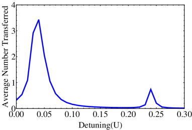
Figure 8: Average fraction transferred of a 6-boson 4-site entangled state driven by the external rf field. The parameters are $U_{a}=U_{ab}=1$, $ZJ=0.05$, $\mu=1.5$, and $U_{b}=\omega_{ba}=5$. We can see the spectrum has 2 peaks with positive shifts of order $J$.

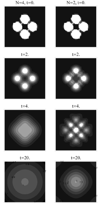
Figure 9: Matter wave interference patterns (per particle contribution). The left column is the 4-particle 4-site Mott-insulator, and the right one is the 2-particle 4-site condensate. The four rows from top to bottom are at $t=0$, $2$, $4$, and $20$ time units($ml^{2}/2\hbar$). All parts of the figure have the same spatial scale. The number in the last row is the relative value of the density.

Turning to the role of the Goldstone modes in rf transitions, the form of the rf perturbation (given in the position basis of the physical particles as $\sum\limits{}_{i}\gamma\hat{a}_{i}^{\dagger}\hat{b}_{i}+h.c.$) is given in the Goldstone basis by

$$H_{rf}= - \sqrt{N}\gamma\hat{B}_{0}^{\dagger}+\frac{{\gamma\sin\theta}}{{4\sqrt{\bar{n}}}}\sum\limits_{p}{(v_{p}+u_{p})\hat{B}_{p}^{\dagger}(\alpha_{p}+\alpha_{-p}^{\dagger})}$$ (35)

$$+ \rm{H.c.},$$

where $N$ is the total number of particles and ${\bar{n}}=n+\cos^{2}(\theta/2)$ is the number density at zero temperature. The first term creates a $B$ boson uniformly in space without any distortions in density or phase (which are represented by $\alpha$ bosons). The second term creates a $B$ boson with momentum $p$ accompanied by an $\alpha$ boson with momentum $-p$ or annihilation of an $\alpha$ boson with momentum $p$.

For the 3D system at zero temperature, using the above Goldstone representation of the rf perturbation in Fermi’s golden rule [(Eq. 12)], we find the transition rate due to the first term of Eq. (35) is $I^{(1)}(\omega)\propto\delta(\omega-\omega_{B})$. This delta peak corresponds to the first peak we obtained in Sec. IIIA, although slightly shifted given the slightly different mean-field energy estimates. The transition rate due to the second term is $I^{(2)}(\omega)\propto\sin^{2}\theta|\omega-\omega_{B}|^{3}$ which is so small compared to the delta function near $\omega_{B}$ that the effect of $I^{(2)}$ on the contrast of $I^{(1)}$ can be ignored. We expect similar argument to hold for the second peak obtained in Sec. III.1. Therefore, we find that excitation of Goldstone modes by a weak rf field will not obscure the two-peak signature at zero temperature. At low temperatures of order $kT\ll ZJ$, the initial state still contains zero $B$ bosons but does contain $\alpha$ bosons (corresponding to Goldstone modes) with a bosonic thermal distribution. Taking these thermally-excited $\alpha$ bosons into consideration in the rf signal, we find that $I^{(1)}$ is still a delta peak, while $I^{(2)}$ becomes a finite function of $|\omega-\omega_{B}|$ which does not obscure the peak $I^{(1)}$. For higher temperatures of order $ZJ$ (when the average number of $\alpha$ bosons per site is of order $1$ or more), the higher order terms in $H_{rf}$ cannot be ignored.

Appendix C Time-evolution of a six-boson four-site system

The dynamics of finite bosons in a small number of lattice sites can be numerically solved without using the mean-field approach, and the results reflect the physical signatures predicted in our theoretical analysis. Here we consider a system of six bosons on four sites located on a ring. The ground state is given by

$$\frac{1}{{2\sqrt{2}}}(\left|1\right\rangle\left|1\right\rangle\left|2\right\rangle\left|2\right\rangle+\left|1\right\rangle\left|2\right\rangle\left|2\right\rangle\left|1\right\rangle+\left|2\right\rangle\left|2\right\rangle\left|1\right\rangle\left|1\right\rangle$$

$$+\left|2\right\rangle\left|1\right\rangle\left|1\right\rangle\left|2\right\rangle)+\frac{1}{2}\left(\left|1\right\rangle\left|2\right\rangle\left|1\right\rangle\left|2\right\rangle+\left|2\right\rangle\left|1\right\rangle\left|2\right\rangle\left|1\right\rangle\right)$$

$$+{\rm O}(J/U),$$ (36)

where $\left|{n_{1}}\right\rangle\left|{n_{2}}\right\rangle\left|{n_{3}}\right\rangle\left|{n_{4}}\right\rangle$ means the state with the $i$th site occupied by $n_{i}$ bosons. The ground state has nonzero single-site number fluctuations, which differentiate the condensate from the Mott-insulator. Thus the system is expected to have an rf spectrum similar to that of a many-particle condensate. We use the Bose-Hubbard Hamiltonian, plus time-dependent terms which represent the interaction with the rf field, to numerically time evolve the ground state, and compute the average number of bosons transferred from the $a$ state to the $b$ state (Fig. 8). The result shows two peaks with shifts of order $J$, as we obtained in Sec. II through the mean-field approach.

To show matter-wave interference, we calculate the density contribution per particle of a two-particle four-site system (condensate) and that of a four-particle four-site system (the Mott-insulator) in free expansion(Fig. 9). Both cases have the same initial density profile but have very different interference patterns in expansion. The condensate shows more interference peaks and has a much higher density in the center at long times than the Mott-insulator does. This difference is similar to the difference between the phase-coherent state (superfluid) and the phase-incoherent state (the Mott-insulator) in the experiment of Ref. Greiner02 .

References

- (1) I. Bloch, J. Dalibard, and W. Zwerger, Rev. Mod. Phys. 80, 885 (2008).
- (2) M. Greiner, Ph.D. thesis, Ludwig-Maximilians- Universitat Munchen (2003).
- (3) M. P. A. Fisher, P. B. Weichman, G. Grinstein, and D. S. Fisher, Phys. Rev. B 40, 546 (1989).
- (4) M. Greiner, O. Mandel, T. Esslinger, T. W. Hansch, and I. Bloch, Nature (London) 415, 39 (2002).
- (5) D. Jaksch, C. Bruder, J. I. Cirac, C. W. Gardiner, and P. Zoller, Phys. Rev. Lett. 81, 3108 (1998).
- (6) B. DeMarco, C. Lannert, S. Vishveshwara, and T.-C. Wei, Physical Review A 71, 063601 (2005).
- (7) P. Rabl, A. J. Daley, P. O. Fedichev, J. I. Cirac, and P. Zoller, Phys. Rev. Lett. 91, 110403 (2003).
- (8) D. Jaksch and P. Zoller, Annals of Physics 315, 52 (2005).
- (9) M. Popp, K.G.H. Vollbrecht, and J. I. Cirac, Fortschr. Phys. 54, No. 8 V 10, 686 V 701 (2006)
- (10) D. van Oosten, P. van der Straten, and H. T. C. Stoof, Physical Review A 63, 053601 (2001).
- (11) E. Taylor and E. Zaremba, Physical Review A 68, 053611 (2003).
- (12) D. van Oosten, D. B. M. Dickerscheid, B. Farid, P. van der Straten, and H. T. C. Stoof, Physical Review A 71, 021601(R) (2005).
- (13) K. Sengupta and N. Dupuis, Physical Review A 71, 033629 (2005).
- (14) G. Pupillo, A. M. Rey, and G. G. Batrouni, Physical Review A 74, 013601 (2006).
- (15) R. A. Barankov, C. Lannert, and S. Vishveshwara, Physical Review A 75, 063622 (2007).
- (16) K. Mitra, C. J. Williams, and C. A. R. Sa de Melo, Physical Review A 77, 033607 (2008).
- (17) C. Menotti and N. Trivedi, Physical Review B 77, 235120 (2008).
- (18) G. K. Campbell, J. Mun, M. Boyd, P. Medley, A. E. Leanhardt, L. G. Marcassa, D. E. Pritchard, and W. Ketterle, Science 313, 649 (2006).
- (19) K. R. A. Hazzard and E. J. Mueller, Physical Review A 76, 063612 (2007).
- (20) S. Folling, A. Widera, T. Muller, F. Gerbier, and I. Bloch, Phys. Rev. Lett. 97, 060403 (2006).
- (21) S. Sachdev, Quantum Phase Transitions, 1st, ed. (Cambridge University Press, Cambridge, 2006).
- (22) W. Zwerger, Journal of Optics B: Quantum and Semiclassical Optics 5, S9 (2003).
- (23) R. Bach and K. Rzazewski, Physical Review A 70, 063622 (2004).
- (24) A. J. Leggett, Quantum Liquids, 1st, ed. (Oxford University Press, Oxford, 2006).
- (25) D. S. Rokhsar and B. G. Kotliar, Phys. Rev. B 44, 10328 (1991).
- (26) K. Sheshadri, H. R. Krishnamurthy, R. Pandit, and T. V. Ramakrishnan, Europhys. Lett. 22, 257 (1993).
- (27) C. Bruder, R. Fazio, and G. Schon, Phys. Rev. B 47, 342 (1993).
- (28) E. Altman and A. Auerbach, Phys. Rev. Lett. 89, 250404 (2002).
- (29) M. R. Matthews, D. S. Hall, D. S. Jin, J. R. Ensher, C. E. Wieman, E. A. Cornell, F. Dalfovo, C. Minniti, and S. Stringari, Phys. Rev. Lett. 81, 243 (1998).
- (30) F. Gerbier, Phys. Rev. Lett. 99, 120405 (2007).
- (31) C. J. Pethick and H. T. C. Stoof, Physical Review A 64, 013618 (2001).
- (32) D.-S. Luhmann, K. Bongs, K. Sengstock, and D. Pfannkuche, Physical Review A 77, 023620 (2008).
- (33) S. Konabe, T. Nikuni, and M. Nakamura, Physical Review A 73, 033621 (2006).
- (34) G. Pupillo, C. J. Williams, and N. V. Prokof’ev, Physical Review A 73, 013408 (2006).
- (35) F. Gerbier, A. Widera, S. Folling, O. Mandel, T. Gericke, and I. Bloch, Phys. Rev. Lett. 95, 050404 (2005).
- (36) F. Gerbier, A. Widera, S. Folling, O. Mandel, T. Gericke, and I. Bloch, Physical Review A 72, 053606 (2005).
- (37) R. Roth and K. Burnett, Physical Review A 67, 031602(R) (2003).
- (38) R. B. Diener, Q. Zhou, H. Zhai, and T.-L. Ho, Phys. Rev. Lett. textbf98, 180404 (2007).
- (39) G.-D. Lin, W. Zhang, and L.-M. Duan, Physical Review A 77, 043626 (2008).
- (40) E. Toth, A. M. Rey, and P. B. Blakie, Physical Review A 78, 013627 (2008).
- (41) D. J. Griffiths, Introduction to Quantum Mechanics, 2nd ed. (Pearson Education, Inc., Upper Saddle River, NJ, 2005).
- (42) C. Lannert, T.-C. Wei, and S. Vishveshwara, Physical Review A 75, 013611 (2007).