Scale-dependent bias induced by local non-Gaussianity: A comparison to N-body simulations
Abstract
We investigate the effect of primordial non-Gaussianity of the local type on the auto- and cross-power spectrum of dark matter haloes using simulations of the CDM cosmology. We perform a series of large N-body simulations of both positive and negative , spanning the range between 10 and 100. Theoretical models predict a scale-dependent bias correction that depends on the linear halo bias . We measure the power spectra for a range of halo mass and redshifts covering the relevant range of existing galaxy and quasar populations. We show that auto and cross-correlation analyses of bias are consistent with each other. We find that for low wavenumbers with the theory and the simulations agree well with each other for biased haloes with . We show that a scale-independent bias correction improves the comparison between theory and simulations on smaller scales, where the scale-dependent effect rapidly becomes negligible. The current limits on from Slosar et al. (2008) come mostly from very large scales and, therefore, remain valid. For the halo samples with we find that the scale- dependent bias from non-Gaussianity actually exceeds the theoretical predictions. Our results are consistent with the bias correction scaling linearly with .
keywords:
cosmology: theory — gravitation — dark matter — galaxies: haloes —1 Introduction
Generic inflationary models based on the slow roll of a scalar field predict a nearly scale-invariant and Gaussian spectrum of primordial curvature fluctuations (see Bartolo et al. 2004 for a review). While the latest measurements of the cosmic microwave background (CMB) anisotropies favour a slightly red power spectrum (Komatsu et al. 2008), no significant detection of primordial non-Gaussianity has been reported as yet from CMB and large-scale structures measurements. Nevertheless, improving the current limits would still strongly constrain mechanisms for the generation of cosmological perturbations.
Non-Gaussianity can be generated by nonlinearities in the relation between the primordial curvature perturbation and the inflaton field (e.g. Salopek & Bond 1990; Gangui et al. 1994), interaction of scalar fields (e.g. Falk et al. 1993) or deviation from the (Bunch-Davies) ground state (e.g. Lesgourgues et al. 1997). A wide class of inflationary scenarios lead to non-Gaussianity of the local type, which depends on the local value of the potential only. In these models, deviation from Gaussianity can be conveniently parametrised by a nonlinear coupling parameter through the relation (e.g. Komatsu & Spergel 2001)
| (1) |
where is the Gaussian part of the curvature perturbation in the matter area. While single inflaton scenarios predict much less than unity, multi-field inflation models can generate (Linde & Mukhanov 1997; Lyth et al. 2003; Creminelli 2003; Dvali et al. 2004; Zaldarriaga 2004; Arkani-Hamed et al. 2004; Alishahiha et al. 2004). Alternatives to inflation, such as cyclic/ekpyrotic model also predict large non-Gaussianity of local type (Creminelli & Senatore 2007, Buchbinder et al. 2008, Lehners & Steinhardt 2008).
Higher order statistics of the curvature perturbation such as the bispectrum can be computed straightforwardly from a perturbative expansion of the homogeneous Robertson-Walker background (e.g. Acquaviva et al. 2003; Maldacena 2003). These statistics are related to those of the CMB temperature anisotropy through the radiation transfer function, which can be computed accurately using, e.g., CMBFAST (Seljak & Zaldarriaga 1996). Thus far, analysis of the CMB bispectrum indicates that the data are fully consistent with Gaussianity, with (Komatsu et al. 2003; Creminelli et al. 2007; Komatsu et al. 2008; Smith et al. 2009; see, however, Yadav & Wandelt 2008 who report a detection at the 2.5 level), providing strong evidence for the quantum origin of the primordial fluctuations.
Large-scale structures offer another route to test for the presence of primordial non-Gaussianity. It has long been recognised that departure from Gaussianity can significantly affect the high mass tail of the dark matter halo distribution (Lucchin & Matarrese 1988; Colafrancesco et al. 1989; Chiu et al. 1998; Robinson & Baker 2000; Matarrese et al. 2000; Mathis et al. 2004, Kang et al. 2007; Grossi et al. 2007). Following this approach, X-ray cluster counts have been used to constrain the amount of non-Gaussianity (e.g. Koyama et al. 1999, Robinson et al. 2000; Willick 2000; Amara & Refregier 2004). Galaxy clustering is also sensitive to the statistical properties of the primeval fluctuations. Indeed, Grinstein & Wise (1986) pointed out early that primordial non-Gaussianity could significantly increase the amplitude of the two-point correlation of galaxies and clusters on large scales. However, recent work has mostly focused on higher order statistics such as the bispectrum (Scoccimarro et al. 2004; Sefusatti & Komatsu 2007).
Dalal et al. (2008) have recently sparked renewed interest in the clustering of rare objects by demonstrating the strong scale-dependent bias arising from primordial non-Gaussianity of the local type. It can be shown that the latter contributes a scale-dependent bias of the form (Dalal et al. 2008; Matarrese & Verde 2008; Slosar et al. 2008)
| (2) |
where is the linear bias parameter, is the Hubble parameter, is the matter transfer function, is the growth factor normalised to in the matter era and is the present-day (linear) critical density threshold. While the derivation of this non-Gaussian bias correction presented in Dalal et al. (2008) and Matarrese & Verde (2008) is strictly valid only for the highest peaks of the density field, the peak-background split argument invoked by Slosar et al. (2008) suggests that eq. (2) should apply to all peaks unrestrictedly, but is only valid in the limit of long wavelength modes so that the background can be approximated as a constant density. Further work has confirmed the basic picture (Afshordi & Tolley 2008; McDonald 2008; Taruya et al. 2008).
Slosar et al. (2008) have applied eq. (2) to constrain the value of using a compilation of large-scale structure data. They find (at 95% confidence level). These limits are competitive with those from WMAP5, (Komatsu et al. 2008) and (Smith et al. 2009), demonstrating the promise of the method. Future all sky surveys could achieve constraints of the order of (Dalal et al. 2008; Afshordi & Tolley 2008; McDonald 2008; Carbone et al. 2008), assuming one knows how to extract maximum information from the data (see, e.g., Slosar 2008). In fact, with sufficient high density of tracers it should be possible to circumvent the sampling variance (which is a serious issue since the non-Gaussian effect is strongest on the largest scales) and alleviate degeneracies with other cosmological parameters, thereby allowing for a potentially huge gains (Seljak 2008).
Still, in order to fully exploit the potential of forthcoming large-scale surveys, the method needs to be tested with large numerical simulations. Thus far, eq. (2) has been validated only using the halo-matter cross-power spectrum (Dalal et al. 2008) and only on very large scales, so its accuracy remains uncertain. It is important to measure the effect in the auto-correlation of dark matter haloes, since the latter gives the strongest constraint on (Slosar et al. 2008). It is also important to extend the analysis to smaller scales, where the peak-background split breaks down, as well as to less biased haloes. The purpose of this paper is to address these issues in more detail. We begin with a brief description of the N-body simulations against which we calibrate the theory (§2). Next, we discuss the mass function and bias of the corresponding halo catalogues and demonstrate the importance of including a scale-independent bias correction in the comparison with the simulations (§3). The main body of the paper is §4, where we study in detail the impact of local non-Gaussianity on the halo-matter and halo-halo power spectrum. We conclude with a discussion of the results in §5.
2 The N-body simulations
Investigating the scale-dependence of the halo bias requires simulations large enough so that many long wavelength modes are sampled. At the same time, the simulations should resolve dark matter haloes hosting luminous red galaxies (LRGs) or quasars (QSOs), so that one can construct halo samples whose statistical properties mimic as closely as possible those of the real data.
In this work, we use a series of large N-body simulations of the CDM cosmology seeded with Gaussian and non-Gaussian initial conditions. The non-Gaussianity is of the “local” form, , where is the Bardeen potential. It is important to note that this local transformation is performed before multiplication by the matter transfer function. is computed with CMBFAST (Seljak & Zaldarriaga 1996) for the WMAP5 best-fitting parameters (Komatsu et al. 2008) : , , , and a normalisation of the curvature perturbations (at Mpc-1) which gives . Five sets of three 10243 simulations, each of which has , were run with the N-body code GADGET2 (Springel 2005). We used the same Gaussian random seed field in each set of runs so as to minimise the sampling variance. We also explored lower values of and ran 2 realisations for each of the non-Gaussian models characterized by and . In all cases the box size is 1600 with a force resolution of 0.04 times the mean interparticle distance. The particle mass of these simulations thus is , enough to resolve haloes down to .
Haloes were identified using the MPI parallelised version of the AHF halo finder which is based on the spherical overdensity (SO) finder developed by Gill, Knebe & Gibson (2004). AHF estimates the local density around each halo centre using a top-hat aperture. The virial mass is defined by the radius at which the inner overdensity exceeds times the background density . Note that is an increasing function of redshift ( at ). We discard poorly resolved haloes and only study those containing at least 34 particles to reduce the error in the mass estimate (Warren et al. 2006). This implies a lower mass limit which is about the typical mass of QSO-hosting haloes at (e.g. Porciani & Norberg 2006) and is a few times smaller than the mass of haloes harbouring LRGs in SDSS (Mandelbaum etal. 2006).
3 halo mass function and bias
3.1 Multiplicity function
Analytic arguments based on the Press-Schechter theory (Press-Schechter 1974; Bond et al. 1991; Sheth & Tormen 1999) predict that the halo mass function is entirely specified by the distribution of first-crossings, or multiplicity function
| (3) |
The peak height , where is the critical linear overdensity for collapse (assumed spherical throughout this paper), is the typical amplitude of fluctuations that produce haloes of mass by redshift . A characteristic mass for clustering, , can then be defined through . For the present cosmology, .
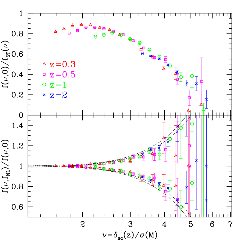
The top panel of Fig. 1 shows the multiplicity function of the SO haloes extracted from the Gaussian simulations at redshift , 0.5, 1 and 2. The numerical data are plotted with respect to the Sheth-Tormen function (Sheth-Tormen 1999) to emphasise the large deviation from the latter. This departure is, however, not really surprising since the Sheth-Tormen formula is a fit to the mass function of Friends-of-Friends haloes (extracted from the GIF simulations, see Kauffmann et al. 1999). We have not attempted to fit the multiplicity function of our SO haloes given the limited volume and dynamic range of our simulations. Instead, we have found more useful to assess whether the impact of local non-Gaussianity on the halo mass function is consistent with theoretical expectations.
To test this we have plotted the ratio in the bottom panel of Fig. 1 for the simulations with . The presence of primordial non-Gaussianity enhances or suppresses the high peak tail of the multiplicity function depending on the sign of . As recognised in previous papers (e.g. Matarrese et al. 2000; Sefusatti et al. 2007), despite the lack of a reliable Gaussian mass function, deviations from Gaussianity can be modelled analytically using the Press-Schechter formalism. Here we follow the simple extension introduced by LoVerde et al. (2008; see also Chiu et al. 1998) and replace the Gaussian probability distribution function (PDF) of the density field by the generic Edgeworth expansion (e.g., Scherrer & Bertschinger 1991; Juskiewicz et al. 1995). Neglecting cumulants other than the skewness and truncating the series expansion at , the non-Gaussian correction factor reads (LoVerde et al. 2008)
| (4) |
after integration over regions above the critical density for collapse. Note that we have omitted the explicit redshift dependence. Strictly speaking however, the ratio depends distinctly upon the variables (or ) and due to the presence of . Our notation is motivated by the fact that the measured non-Gaussian correction, as plotted in the bottom panel of Fig. 1, appears to depend mostly on the peak height.
Equation (4) requires knowledge of the skewness of the smoothed density field , which we compute analytically using the relation (see Appendix §A)
where , is the power spectrum of linear curvature perturbations in the matter-dominated era,
| (6) |
and is a (spherically symmetric) window function of characteristic mass scale . Over the mass range probed by our simulations, , is a monotonic decreasing function of that varies in the narrow range for the top-hat filter assumed here. Furthermore, the term dominates the total contribution to the non-Gaussian correction when the peak height is .
The resulting non-Gaussian correction is plotted in the bottom panel of Fig. 1 for two different redshifts, (dotted) and 2 (dotted-dashed). The truncated expansion eq. (4) agrees reasonably well with the numerical data, suggesting thereby that cumulants higher than may not be important in the range of mass and redshift considered here. Note also that for positive the mass function is enhanced more at the high mass end and that this is similar to an increase in the amplitude of fluctuations . Hence, is somewhat degenerate with since, in both cases, the effect increases with mass (compare with Fig.3 of Mandelbaum & Seljak 2007 for instance). However, at (i.e. at ) the increase in mass function for is 15%, which corresponds to less than 0.01 change in . Therefore, given the current uncertainties in the cluster abundance (which translate into 0.03 error on , Vikhlinin et al. 2008), the prospects of using halo mass function to place competitive limits on with the current data are small.
3.2 Linear bias
Having checked that the level of non-Gaussianity in the mass function is consistent with simple theoretical expectations, we now turn to the clustering of dark matter haloes.
We interpolate the dark matter particles and halo centres onto a regular cubical mesh. The resulting dark matter and halo fluctuation fields, and , are then Fourier transformed to yield the matter-matter, halo-matter and halo-halo power spectra , and , respectively. Notice that the power spectra are computed on a 5123 grid to reduce the computational expenses. Still, the Nyquist wavenumber is sufficiently large, , to allow for an accurate measurement of the power in wavemodes of amplitude . As we will see shortly, the impact of local non-Gaussianity is negligible at , but increases rapidly with decreasing wavenumber.
On linear scales, the halo bias approaches a constant, albeit mass-dependent value . The linear halo bias needs to be measured accurately as it controls the strength of the scale-dependent bias correction induced by local non-Gaussianity. To proceed, we may consider the following estimates of for a given halo sample,
| (7) |
In the following, we will always correct the halo power spectrum for shot-noise, which we assume to be if dark matter haloes are a Poisson sampling of some continuous field. While this discreteness correction is negligible for and due to the large number of dark matter particles, it can be quite significant for .
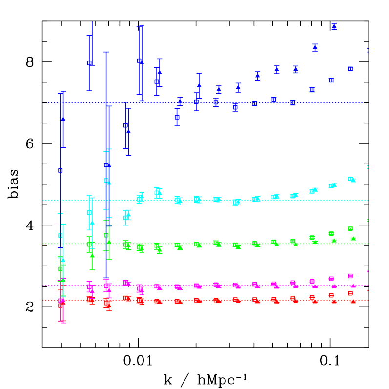
In Fig. 2, the result of measuring and in the Gaussian simulations is shown at various redshifts for the haloes of mass . Error bars indicate the scatter among the various realisations. Except for the most biased sample, and are nearly constant and agree well with each other when the wavenumber varies in the “linear” range . On these scales, the slight offset between and suggests that the shot-noise correction might be too large for the low bias haloes and too small for the highest bias halo. It is worth pointing out that the hypothesis of shot noise being for the dark matter haloes remains unproven (McDonald 2008) and it is an issue worth exploring further. Here we will be mostly looking at ratios of power spectra with and without non-Gaussianity, so this is less of an issue. Both bias quantities feature some scale-dependence on smaller scales, . This is best seen in the most biased sample. We will use as a proxy for the linear halo bias since it is less sensitive to shot-noise. In Fig. 2, the horizontal lines indicate our fit to obtained from the measurement of at wavenumber .
3.3 Non-gaussian bias shift
As shown in Dalal et al. (2008), Matarrese & Verde (2008) and Slosar et al. (2008), local non-Gaussianity gives rise to the scale-dependent bias correction eq. (2). However, at the lowest order there are two additional, albeit relatively smaller, corrections which arise from the dependence of both the halo number density and the matter power spectrum on . As we will see shortly, the inclusion of these extra terms substantially improves the comparison between the theory and the simulations.
Firstly, assuming the peak-background split holds, the change in the mean number density of haloes induces a scale-independent shift which we denote by . The existence of such a term was noted in Slosar et al. (2008) and Afshordi & Tolley (2008). Using the non-Gaussian fractional correction eq. (4) (which is not universal), this contribution reads
This approximation should work reasonably well for moderate values of the peak height, , for which the formula of LoVerde et al. (2008) matches well our data (see Fig. 1). It is worth noticing that has a sign opposite to that of (because the bias decreases when the mass function goes up). In practice, to estimate for a given halo sample, we evaluate and at the scale corresponding to the average halo mass of the sample. Furthermore, since we consider only first order corrections to the Gaussian bias, we set in the above expression so that is truly first order in .
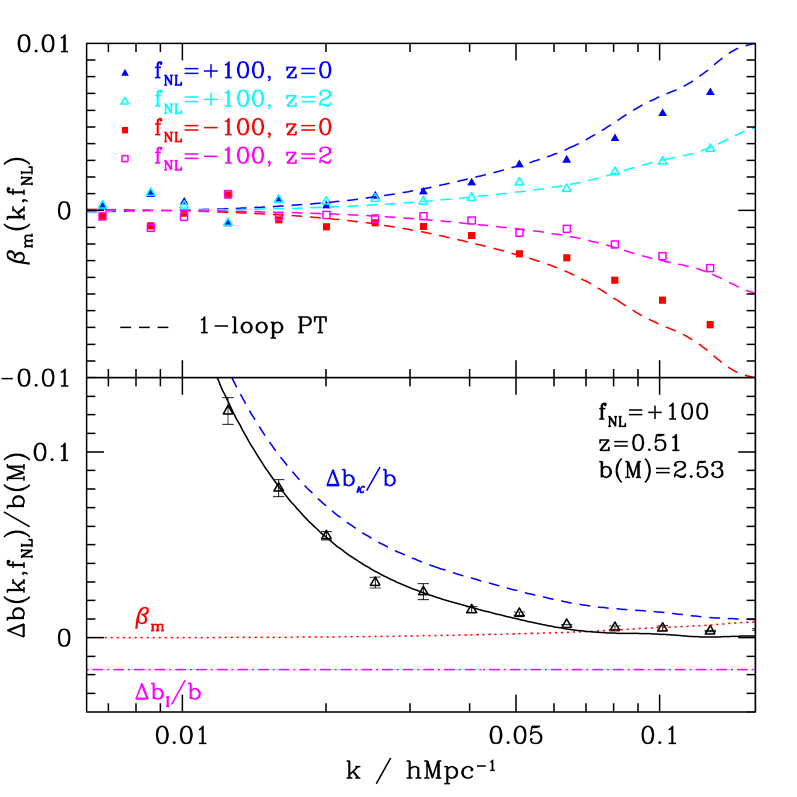
Secondly, primordial non-Gaussianity affects the matter power spectrum as positive values of tend to increase the small-scale power (Scoccimarro et al. 2004; Grossi et al. 2008; Taruya et al. 2008). For , the magnitude of this correction is at a per cent level in the weakly nonlinear regime . In order to illustrate this effect, the top panel of Fig. 3 displays the deviation that arises from the presence of primordial non-Gaussianity of the local type. The symbols show the result of measuring this ratio from the snapshots at redshift and 2, whereas the dashed curves show the prediction from one-loop perturbation theory (Taruya et al. 2008; see also Appendix §A). As we can see, leading order perturbation theory (PT) provides an excellent description of the effect over the wavenumbers of interest, . At , one-loop PT overestimates the non-Gaussian correction by per cent for and it is possible the agreement could be improved further using renormalised perturbation theory (see, e.g., Crocce & Scoccimarro 2008).
Summarizing, local non-Gaussianity adds a correction to the bias of dark matter haloes that can be written as
| (9) |
at first order in . The bottom panel of Fig. 3 illustrates the relative contribution of these terms for haloes of mass identified at redshift . The solid curve shows the total non-Gaussian bias . Considering only the scale-dependent shift leads to an apparent suppression of the effect in simulations relative to the theory. Including the scale-independent correction considerably improves the agreement at wavenumbers . Finally, adding the scale-dependent term further adjusts the match at small scale by making the non-Gaussian bias shift less negative.
4 Results
In order to quantify the effect of non-Gaussianity on the halo bias, we will consider the ratios 111Strictly speaking, is equal to , which differs from eq. (10) by . In what follows however, we will use for notational convenience.
| (10) | |||||
Moreover, we shall also quantify the departure from the theory as a function of wavemode amplitude with the ratio . Here, is the non-Gaussian bias correction measured from the simulation whereas is the theoretical scaling eq. (9).
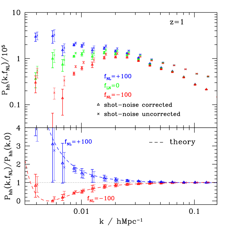
Before proceeding we look at the effect of the shot-noise correction on the measurement of the non-Gaussian bias . In Fig. 4, the averaged halo power spectrum and the ratio are shown before and after applying the discreteness correction. Error bars represent the scatter among the realisations. The bias and the number density of the halo sample considered here is and , respectively.
As we can see, the shot-noise can have a non-negligible effect on the largest scales, specially for the haloes extracted from the simulations with for which the large scale power crosses zero on very large scales. For this particular sample, the shot-noise correction enhances the measurement of by 10-15 per cent at scales , regardless of the sign of . While the exact amount of correction depends upon the bias and the number density of the halo sample under consideration, it is clear that any attempt to measure at the few per cent level must include the discreteness correction.
4.1 Non-Gaussian bias from the halo-halo and halo-matter power spectra
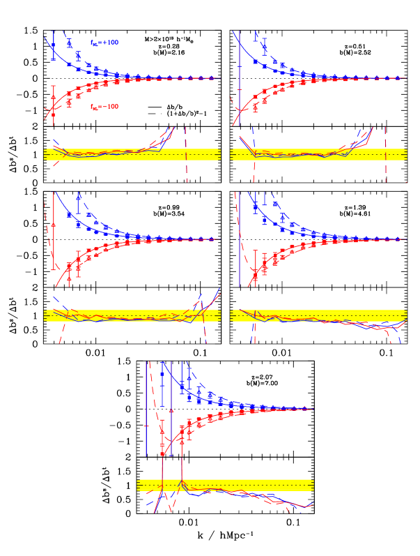
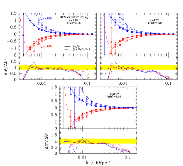
We have measured power spectra for a range of halo masses and redshifts, covering the relevant range of statistical properties corresponding to the available data sets of galaxies or quasar populations with different luminosities and bias. The results are summarised in Figures 5 and 6, where the averaged and are plotted as a function of wavenumber. The deviation from the theoretical prediction, , is also shown at the bottom of each panel. The shaded region indicates a deviation less than 20 per cent. To reduce the impact of sampling variance, we first compute the ratios and for each realisation, and then average over the realisations (see, e.g., Smith et al. 2007). We note that reversing the sequence of operations, i.e. taking the ratio of averaged power spectra, gives very similar average values. Error bars denote the scatter around the mean and, therefore, may underestimate the true errors since they are computed from a small number of realisations.
As we can see, the theoretical prediction provides a very good description of the simulations at small wavenumber , but the ratio differs significantly from unity at larger wavenumbers. The exact amount of deviation depends weakly on the sign of . For moderately biased haloes with the theory approaches the numerical results already on scale . For the highly biased samples , the theory overpredicts the effect seen in simulations on all scales, but somewhat more on smaller scales, although in the high bias limit the numerical data is noisier due to the very low number density of haloes. It is worth noticing that, at the largest scales , the cross-power spectrum goes negative while remains positive and even increases, in good agreement with the analytic prediction.
We suspect these deviations at high wavenumber are mostly due to the breakdown of the peak-background split approximation which was used in the derivation of the scale-dependent bias term in Slosar et al. (2008). For this approximation to be valid one assumes that the long wavelength modes act as a homogeneous change of the background, from which the effect of the non-Gaussianity is computed by comparing it to the local rescaling of the fluctuation amplitude. Clearly this assumption breaks down once the wavelength of the mode becomes small. Uncertainties in the scale-independent correction also affect . In this paper we use analytic predictions based on equation (3.3), but we could also treat the scale-independent bias as a free parameter that we fit to the data, as done in the actual data analysis of Slosar et al. 2008. For example, a per cent smaller (larger) at () would noticeably improve the convergence at large . Finally, notice that the auto- and cross-power spectrum of haloes give comparable results at all but the (poorly sampled) largest scales, where sampling variance prevents us from making any conclusions. This confirms the validity of the analysis in Slosar et al. (2008), where this effect was applied to the auto-correlations of galaxies and quasars.
To assess the extent to which the agreement between simulation and theory depends upon the halo mass and bias, Figures 6 and 7 further explore the effect in the low and high redshift outputs. In Fig. 6, the non-Gaussian bias is shown for haloes that correspond more closely to the quasars used by Slosar et al. (2008), which are at and with . Our halo samples span a similar redshift range, . However, the mass cut gives larger values of the bias, , suggesting that the quasars are hosted by haloes (slightly) less massive than (unresolved in our simulations). As can be seen, the correction factor is similar to that of the samples at high redshift (cf. Fig. 5).
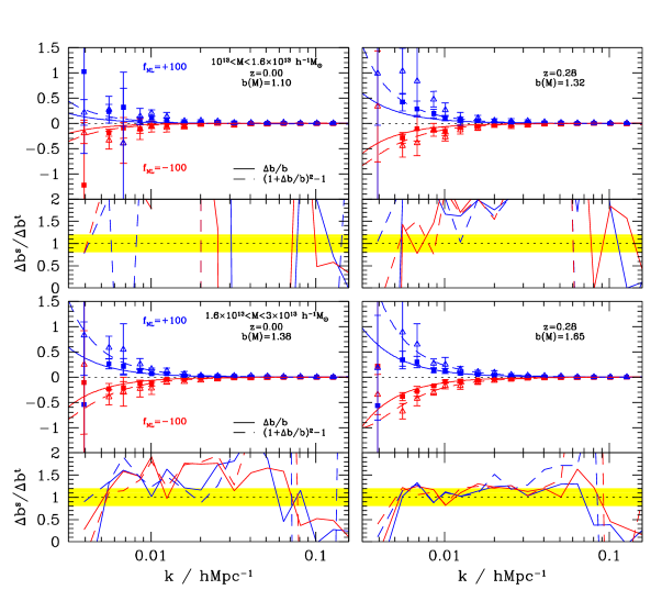
For the redshift outputs , the relatively large number of dark matter haloes allows us to split the catalogues into several non-overlapping subsamples having a number density . For these snapshots, we consider the mass bins , and . Results are shown in Fig. 6. An increase in the ratio as a function of wavenumber followed by a change of sign can also be seen in these low biased samples in spite of the noisier data. Notice that the linear halo bias is in the range . In particular, the haloes with mass constitute an almost unbiased sample of the density field, with . At scales there is some evidence that the non-Gaussian bias correction measured in the low biased samples may be larger than the theoretical expectation. Still, the bias shift is quite small for , in agreement with the theoretical prediction that the effect vanishes for assuming the Eulerian bias prescription (where is the Lagrangian bias) used in eq. (9). Unfortunately, our simulations do not have sufficient mass resolution to resolve anti-biased haloes with , for which theoretical predictions based on the peak-background split suggest the sign of the scale-dependent contribution is reversed.
We have not examined the behaviour of at since the effect is already quite small there and nonlinear bias due to galaxy evolution effects dominates. Most of the information on the non-Gaussian bias comes from measurements at large scale (see Slosar et al. 2008), where the theoretical model and the numerical data agree reasonably well with each other over the relevant range .
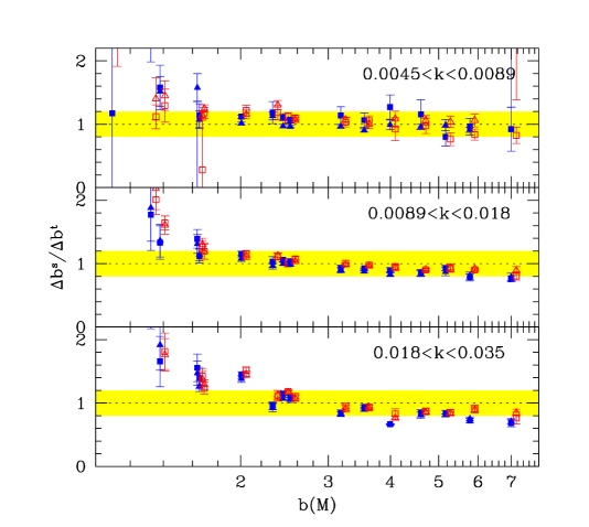
To reduce the scatter in the measurement of , we can increase the bin width so as to increase the number of independent modes. In Fig. 8, the ratio is shown as a function of the linear halo bias for three equally spaced logarithmic interval spanning the range (e.g. ). The data points are harvested from several outputs spanning the redshift range (i.e., the snapshot redshifts are , 0.3, 0.5, 1, 1.4, 1.7 and 2). The squares and triangles represent the deviation from the theoretical prediction obtained by taking ratios of and , respectively. Filled symbols show results for the non-Gaussian simulations with . The error bars indicate our jackknife error estimates on the average .
The non-Gaussian bias shift of the low biased samples, , appears to deviate from the theory. Equation (9) may thus need correction when the linear bias gets lower than . The scale-dependent bias is quite large around , although for the effect does appear to vanish on the largest scales as expected (see the upper left panel of Fig. 7). For the haloes with , the theory matches the non-Gaussian bias correction for . One would need even larger simulation boxes than used here to properly sample the largest scales. For , the effect is slightly suppressed compared to the theoretical prediction, but this may plausibly arise from uncertainties in the magnitude of the theoretical scale-independent shift . Indeed, we have found that a 20 per cent increase in considerably improves the agreement for and, at the same time, is still consistent with the measured fractional change in the multiplicity function (see Fig. 1). Finally, note that that haloes with similar bias also have a comparable scale-dependent bias due to non-gaussianity regardless of redshift. Hence, there is no need to introduce a second parameter such as redshift for the purpose of describing these results.
The only previous work with simulations along these lines is that of Dalal et al. (2008). These authors do not include the scale-independent shift nor the weaker correction induced by the matter power spectrum. Hence, Fig. 8 of their paper indeed shows . This ratio appears to increase with wavenumber (even though their data points do not extend beyond ), while the bottom panel of our Fig. 4 shows that is suppressed at high wavenumbers. Note, however, that their theoretical scale-dependent correction does not include the matter transfer function. We found that, if the transfer function were removed from eq. (2), would be enhanced rather than suppressed as one goes to higher wavenumber, in qualitative agreement with their findings. Since the non-Gaussianity is imprinted in the initial conditions prior to the evolution through matter and radiation domination, the transfer function must be included in the analysis.
4.2 Scaling with
The quadratic term also induces second and higher order corrections to the effective bias shift which may become important at high wavenumber. To test for these high order terms, we explore in Fig. 9 the scaling of the non-Gaussian bias shift with the strength of the nonlinear parameter . Symbols show the ratio (which we abridge for shorthand convenience) as a function of wavenumber and redshift for several values of and spanning the range [-100,+100], as indicated in the figure. Note that the data points are obtained by averaging over two realisations only. The horizontal line indicates the value that should be reached if the non-Gaussian bias shift is linear in .
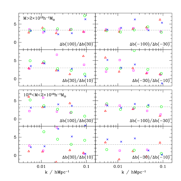
As we can see, there is less scatter in than in but, in both cases, the results are broadly consistent with the linear expectation . Furthermore, there is no significant dependence on the wavenumber, redshift or the halo mass cut. We conclude that the sensitivity of large scale structure bias should extend to smaller values of as expected.
4.3 Non-Gaussian bias in configuration space
Thus far, we have investigated the impact of local non-Gaussianity on two-point statistics in Fourier space. It is also instructive to consider the two-point correlation in configuration space, which is related to the power spectrum through
| (11) |
where is the zeroth spherical Bessel function. In practice, since the simulation volume is a periodic cube, we compute the correlation from a discrete Fourier transform of the power spectrum.
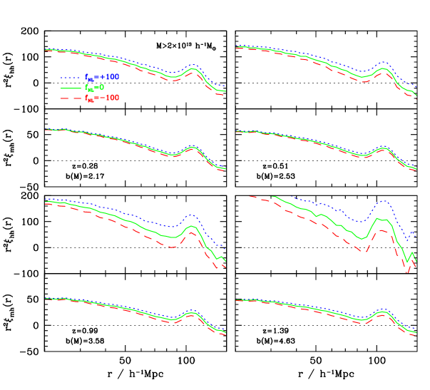
In Fig. 10, the result of measuring the auto and cross-correlation functions is shown at for the mass cut . The width of the simulation box is large enough to sample wavemodes relevant to the baryon acoustic oscillations (BAO). The interesting feature of Fig. 10 is the correlation between the BAO and the broadband power, which shows up differently in the correlation function than in the power spectrum. Local non-Gaussianity adds broadband power and, therefore, modulates the amplitude of the BAO and the position of zero-crossing.
5 Discussion and conclusions
The scale dependence of clustering of biased tracers of the density field has emerged as a powerful method to constrain the amount of primordial non-Gaussianity of the local type. In this paper, we have measured the non-Gaussian bias correction in the clustering of dark matter haloes extracted from a suite of large N-body simulations. In contrast to previous work, we focus both on the halo-halo and halo-matter power spectrum. While we confirm the basic effect reported in Dalal et al. (2008), we emphasize the importance of including a scale-independent term and, to a lesser extent, a contribution induced by the matter power spectrum , to the scale-dependent shift when comparing the theoretical scaling to numerical simulations. The inclusion of these two first order corrections significantly improves the agreement at wavenumber .
The original analysis in Dalal et al. (2008) only used cross-power spectra from simulations, while the data analysis in Slosar et al. (2008) used mostly auto-power analysis. The two do not have to agree with each other if the haloes and dark matter do not trace each other on large scales, i.e. if there is stochasticity. While models with Gaussian initial conditions predict there is little stochasticity on large scales (Seljak & Warren 2004), this has not been shown explicitly for models with non-Gaussianity. Hence, one of the main motivations for this work was to extract the non-Gaussianity effect from the auto-correlations. Measurements of the non-Gaussian bias correction obtained with the halo-halo or the halo-matter power spectrum are in a good agreement with each other, indicating that non-Gaussianity does not induce stochasticity and the predicted scaling applies equally well for the auto- and cross-power spectrum. The issue of stochasticity in non-gaussian models will be explored further in a future publication.
For biased haloes (), our results indicate that the simulated non-Gaussian bias converges towards the theoretical prediction for . At smaller scales, the effect depends on scale-independent bias. If it is ignored then the amplitude of the effect is suppressed relative to theory. If we include scale independent bias using analytic calculation this suppression is much smaller and in some cases goes in the opposite direction. Moreover, one could argue that scale-independent bias cannot be identified from the data alone, so one should fit for it and include it in the overall bias, as was done in Slosar et al. 2008. In this case the agreement between theory and simulations is improved further. Still, there is some evidence that for very biased haloes, , the effect is suppressed relative to theory even on very large scales.
For the halo samples with there is some evidence that the actual bias exceeds the theory on all scales. Therefore, the proposed eq. (9) does not appear to be universal, so care must be exercised when applied to the actual large scale structure data. It would be useful to verify eq. (9) on dark matter haloes which are anti-biased () relative to the matter distribution, to see if the sign of the effect is reversed. One, however, needs a very large volume and a very high mass resolution, which prevents us from verifying the predictions in this regime with the current simulations.
On the observational side, Slosar et al. (2008) have already applied the method to a sample of highly biased LRGs and QSOs, with mean bias and 2.7, respectively. It is interesting to inspect how those constraints change in light of our analysis. Our results suggest that for these values of halo bias theory and simulations are largely in agreement on relevant scales: their constraints arise mostly from the measurement of the quasar power spectrum with at the largest angular scales, and from LRGs with at . As we see from Fig. 8, theoretical predictions are in very good agreement with the simulations for these values of bias and scales. Hence, we thus expect their limits remain unchanged.
Finally, we note that we have not considered other effects that may also modify the predictions, such as redshift space distortions and merger bias. The latter can significantly weaken the predicted scale-dependent bias (Slosar et al. 2008). We plan to investigate these effects with simulations in the future.
Acknowledgements
We are indebted to Volker Springel and Alexander Knebe for making their code, resp. GADGET2 and AMIGA, available. We thank Pat McDonald and Robert Smith for useful discussions and Chris Hirata for pointing out to us the importance of scale-independent bias. The simulations used in this paper were run on the zBOX3 supercomputer at the University of Zürich. We acknowledge support from the Swiss National Foundation (Contract No. 200021-116696/1).
References
- [1] Acquaviva V., Bartolo N., Matarrese S., Riotto A., 2003, Nucl. Phys. B, 667, 119
- [2] Afshordi N., Tolley A.J., 2008, Phys. Rev. D, 78, 123507
- [3] Alishahiha M., Silverstein E., Tong D., 2004, Phys. Rev. D, 70, 123505
- [4] Amara A., Refregier A., 2004, MNRAS, 351, 375
- [5] Arkani-Hamed N., Creminelli P., Mukohyama S., Zaldarriaga M., 2004, J. Cosmo. Astropart. Phys., 4, 1
- [6] Bartolo N., Komatsu E., Matarrese S., Riotto A., 2004, Physics Reports, 402, 103
- [7] Bond J.R., Cole S., Efstathiou G., Kaiser N., 1991, ApJ, 379, 440
- [8] Buchbinder, E. I., Khoury, J., Ovrut, B. A., 2008, Phys. Rev. Lett. 100, 1302
- [9] Carbone C., Verde L., Matarrese S., 2008, ApJ, 684, L1
- [10] Chiu W.A., Ostriker J.P., Strauss M.A., 1998, ApJ, 494, 479
- [11] Colafrancesco S., Lucchin F., Matarrese S., 1989, ApJ, 345, 3
- [12] Creminelli P., 2003, J. Cosmo. Astropart. Phys., 10, 3
- [13] Creminelli P., Senatore, L., 2007, J. Cosmo. Astropart. Phys., 11, 10
- [14] Creminelli P., Senatore L., Zaldarriaga M., Tegmark M., 2007, J. Cosmo. Astropart. Phys., 03, 005
- [15] Crocce M., Scoccimarro R., 2008, Phys. Rev. D, 77, 023533
- [16] Dalal N., Doré O., Huterer D., Shirokov A., 2008, Phys. Rev. D, 77, 123514
- [17] Dvali G., Gruzinov A., Zaldarriaga M., 2004, Phys. Rev. D, 69, 023505
- [18] Falk T., Rangarajan R., Srednicki M., 1993, ApJ, 403, L1
- [19] Gill S.P.D., Knebe A., Gibson B.K., 2004, MNRAS, 351, 399
- [20] Goroff M.H., Grinstein B., Rey S.-J., Wise M.B., 1986, ApJ, 311, 6
- [21] Grinstein B., Wise M.B., 1986, ApJ, 310, 19
- [22] Grossi M., Dolag K., Branchini E., Matarrese S., Moscardini L., 2007, MNRAS, 382, 1261
- [23] Grossi M., Branchini E., Dolag K., Matarrese S., Moscardini L., 2008, MNRAS, 390, 438
- [24] Gangui A., Lucchin F., Matarrese S., Mollerach S., 1994, ApJ, 430, 447
- [25] Jain B., Bertschinger E., 1994, ApJ, 431, 495
- [26] Juskiewicz R., Weinberg D.H., Amsterdamski P., Chodorowski M., Bouchet F.R., 1995, ApJ, 442, 39
- [27] Kang X., Norberg P., Silk J., 2007, MNRAS, 376, 343
- [28] Kauffmann G., Colberg J.M., Diafero A., White S.D.M, 1999, MNRAS, 303, 188
- [29] Komatsu E., Spergel D.N., 2001, Phys. Rev. D, 63, 063002
- [30] Komatsu E., et al. , 2003, ApJS, 148, 119
- [31] Komatsu E., et al. , 2009, ApJS, 180, 330
- [32] Koyama K., Soda J., Taruya A., 1999, MNRAS, 310, 1111
- [33] Lehners, J., Steinhardt, P. J. 2008, Phys. Rev. D 77, 063533
- [34] Lesgourgues J., Polarski D., Starobinsky A.A., 1997, Nucl. Phys. B, 597, 479
- [35] Linde A., Mukhanov V., 1997, Phys. Rev. D., 56, 535
- [36] LoVerde M., Miller A., Shandera S., Verde L., 2008, J. Cosmo. Astropart. Phys., 04, 014
- [37] Lucchin F., Matarrese S., 1988, ApJ, 330, L535
- [38] Lyth D.H., Ungarelli C., Wands D., 2003, Phys. Rev. D, 67, 023503
- [39] Makino N., Sasaki M., Suto Y., 1992, Phys. Rev. D, 46, 585
- [40] Maldacena J., 2003, JHEP, 5, 13
- [41] Mandelbaum R., Seljak U., Cool R.J., Blanton M., Hirata C.M., Brinkmann J., 2006, MNRAS, 372, 758
- [42] Mandelbaum R., Seljak U., 2007, J. Cosmo. Astropart. Phys., 06, 024
- [43] Matarrese S., Verde L., Jimenez R., 2000, MNRAS, ApJ, 541, 10
- [44] Matarrese S., Verde L., 2008, ApJ, 677, L77
- [45] Mathis H., Diego J.M., Silk J., 2004, MNRAS, 353, 681
- [46] McDonald P., 2008, Phys. Rev. D, 78, 123519
- [47] Porciani C., Norberg P., 2006, MNRAS, 371, 1824
- [48] Press W.H., Schechter P., 1974, ApJ, 187, 425
- [49] Robinson J., Gawiser E., Silk J., 2000, ApJ, 532, 1
- [50] Robinson J., Baker J.E., 2000, MNRAS, 311, 781
- [51] Salopek D.S., Bond J.R., 1990, Phys. Rev. D., 42, 3936
- [52] Scherrer R.J., Bertschinger E., 1991, ApJ, 381, 349
- [53] Scoccimarro R., Sefusatti E., Zaldarriaga M., 2004, Phys. Rev. D, 69, 103513
- [54] Sefusatti E., Vale C., Kadota K., Frieman J. 2007, ApJ, 658, 669
- [55] Sefusatti E., Komatsu E., 2007, Phys. Rev. D, 76, 083004
- [56] Seljak U., Zaldarriaga M., 1996, ApJ, 469, 437
- [57] Seljak U., 2009, Phys. Rev. Lett., 102, 021302
- [58] Seljak U., Warren, M. 2004, MNRAS, 355, 129
- [59] Sheth R.K., Tormen G., 1999, MNRAS, 308, 119
- [60] Slosar A., Hirata C.M., Seljak U., Ho S., Padmanabhan N., 2008, J. Cosmo. Astropart. Phys., 08, 031
- [61] Slosar A., 2009, J. Cosmo. Astropart. Phys., 03, 004
- [62] Smith R.E., Scoccimarro R., Sheth R.K., 2007, Phys. Rev. D, 75, 063512
- [63] Smith K.M., Senatore L., Zaldarriaga M., 2009, ArXiv:0901.2572
- [64] Springel V., 2005, MNRAS, 364, 1105
- [65] Taruya A., Koyama K., Matsubara T., 2008, ArXiv:0808.4085
- [66] Vikhlinin A., et al. , 2009, ApJ, 692, 1060
- [67] Warren M.S., Abazajian K., Holz D.E., Teodoro L., 2006, ApJ, 646, 881
- [68] Willick J.A., 2000, ApJ, 530, 80
- [69] Yadav A.P.S., Wandelt B.D., 2008, Phys. Rev. Lett., 100, 181301
- [70] Zaldarriaga M., 2004, Phys. Rev. D, 69, 043508
Appendix A Perturbation theory with local non-Gaussianity
A.1 Skewness parameter
In non-Gaussianity, the Fourier mode of the curvature perturbation (after matter-radiation equality) is given by
| (12) |
where is the unperturbed Gaussian field with power spectrum . The primordial bispectrum of curvature perturbations is
| (13) |
Hence, the three-point correlation of the Fourier modes of the smoothed matter density field, , reads
| (14) | |||||
where for shorthand convenience. Here, is the Dirac delta and the transfer function is given by eq. (6). Note that we have omitted the explicit redshift dependence of and for brevity. The (connected) three-point function of in configuration space is the Fourier transform of . In particular, the third-moment of the smoothed density field is
| (15) | |||||
We have used the momentum conservation implied by the Dirac delta, i.e. , to obtain the second line. Eq. (3.1) follows after taking advantage of the invariance under the exchange of with and integrating out some of the angular variables.
A.2 Matter power spectrum
Following Taruya et al. (2008), we estimate the non-Gaussian correction to the matter power spectrum in the weakly nonlinear range, , using perturbation theory. At the first order, the matter power spectrum can be expressed as
| (16) | |||||
Here, is the growth factor, is the linear power spectrum of the density field,
are the standard one-loop contributions in the case of Gaussian initial conditions (e.g. Goroff et al. 1986; Makino et al. 1992; Jain & Bertschinger 1994) and
| (19) | |||||
where , is the leading-order correction due to local non-Gaussianity which arises from the non-zero primordial bispectrum of curvature perturbations. is the function eq.(6) with filtering kernel . The particular redshift dependence of these power spectra follows from the assumption of growing-mode initial conditions. The relative contribution of local non-Gaussianity thus is
| (20) |
at leading order. Notice that this ratio scales as , so the effect of local non-Gaussianity on the matter power spectrum is largest at low redshift.