The rotation rate of the solar radiative zone

Abstract

The rotation rate of the solar radiative zone is an important diagnostic for angular-momentum transport in the tachocline and below. In this paper we study the contribution of viscous and magnetic stresses to the global angular-momentum balance. By considering a simple linearized toy model, we discuss the effects of field geometry and applied boundary conditions on the predicted rotation profile and rotation rate of the radiative interior. We compare these analytical predictions with fully nonlinear simulations of the dynamics of the radiative interior, as well as with observations. We discuss the implications of these results as constraints on models of the solar interior.

1 Introduction

Helioseismic inference of the rotation profile of the solar interior has revealed two spatially-distinct regions: an outer differentially-rotating shell surrounding an inner uniformly rotating core (Christensen-Dalsgaard & Schou, 1988; Kosovichev, 1988; Brown et al. 1989; Dziembowski et al. 1989). The transition between the two regions, the solar tachocline, is located precisely at the base of the solar convection zone. It is surprisingly sharp with an average width no larger than a few percent of the solar radius (Charbonneau et al. 1999, Elliott & Gough, 1999). Our understanding of this peculiar rotation profile has steadily marched on in the past three decades, benefiting greatly from the high-performance computing revolution. Today, the field is ripe for more quantitative comparisons between models and observations, and has begun focusing on specific reference points, such as the overall pole-to-equator difference in the rotation rate, the inclination of the isorotation contours, the thickness of the tachocline and finally, the subject of this paper, the rotation rate of the radiative interior.

If one assumes that the solar interior is in a dynamically quasi-steady state, then the rotation rate of the radiative zone $\Omega_{\rm rz}$ can be thought of as a weighted average of the rotation profile observed near the base of the convection zone:

$$\Omega_{\rm cz}(\theta)\simeq\Omega_{\rm eq}(1-a_{2}\cos^{2}\theta-a_{4}\cos^{4}\theta)\mbox{ , }$$ (1)

where $\Omega_{\rm eq}/2\pi=463{\rm nHz}$, $a_{2}=0.17$ and $a_{4}=0.08$ (Schou et al. 1998; Gough 2007). Hence we can formally write

$$\Omega_{\rm rz}=\int_{0}^{\pi/2}W(\theta)\Omega_{\rm cz}(\theta)\sin\theta{\rm d}\theta\mbox{ , }$$ (2)

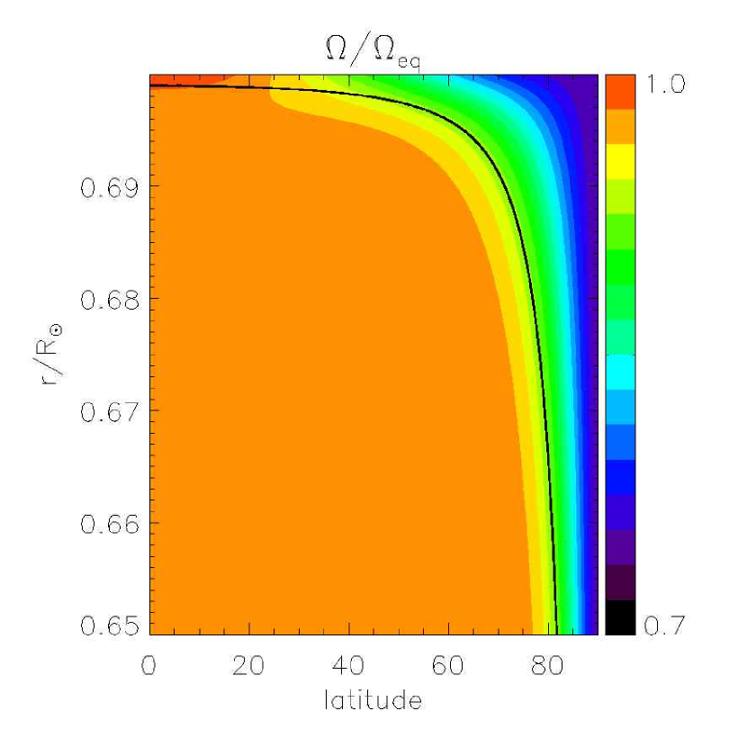
where the weight function $W(\theta)$ depends uniquely on the nature of angular-momentum transport in the tachocline. Observations provide us with relatively precise measurements of $\Omega_{\rm rz}$ (Schou et al. 1998), with

$$\Omega_{\rm rz}/2\pi=430{\rm nHz}\rightarrow\Omega_{\rm rz}\simeq 0.93\Omega_{\rm eq}\mbox{ . }$$ (3)

Can this information be used to constrain theoretical models of the solar interior?

If angular-momentum transport in the radiative zone and the tachocline were purely viscous, the rotation rate of the deeper regions ($r\rightarrow$ 0) would be the same as that of the mean specific angular momentum of the convection zone (Gilman, Morrow & DeLuca, 1989), or in other words $W_{\rm visc}(\theta)=\sin^{2}\theta$ so that

$$\Omega_{\rm visc}=\left(1-\frac{a_{2}}{5}-\frac{3a_{4}}{35}\right)\Omega_{\rm eq}\simeq 0.959\Omega_{\rm eq}\mbox{ . }$$ (4)

Of course, purely viscous transport cannot account for the observed uniform rotation. Spiegel & Zahn (1992) proposed the first tachocline model, in which angular momentum is primarily transported by anisotropic turbulence. Since the stratification of the radiative zone strongly inhibits radial fluid motions, they modelled the effects of this turbulence as a dominantly horizontal diffusion process, and found that the interior would indeed relax to uniform rotation beneath the tachocline with an angular velocity

$$\Omega_{\rm SZ}=\left(1-\frac{3a_{2}}{7}-\frac{5a_{4}}{21}\right)\Omega_{\rm eq}\simeq 0.908\Omega_{\rm eq}\mbox{ . }$$ (5)

Gough & McIntyre (1998, GM98 hereafter) later argued against this model on the ground that two-dimensional turbulence does not act to diffuse angular momentum horizontally (e.g. Tobias, Diamond & Hughes 2007). Moreover, the predicted value $\Omega_{\rm SZ}$ is sufficiently far from the observed value to be ruled out by the observations.

In the past decade, magnetized models have become more widely accepted as the simplest explanation for the observed uniform rotation of the radiative zone (Rüdiger & Kitchatinov 1997; GM98; see Garaud, 2007 for a review). A large-scale primordial magnetic field, strictly confined beneath the convection zone can indeed robustly maintain a state of uniform rotation through Ferraro’s law of isorotation (Ferraro, 1937). The confinement of the primordial field is thought to result from interactions with large-scale meridional flows originating from the convection zone, as originally proposed by GM98, and first shown numerically by Garaud & Garaud (2008) (GG08 hereafter).

However, little attention has been given so far to the predicted rotation rate of the radiative zone in these models. The linear simulations of Rüdiger & Kitchatinov (1997), which assume a given confined poloidal field structure, suggest that $\Omega_{\rm rz}\simeq 0.97\Omega_{\rm eq}$, a value which is much larger than observations. The nonlinear simulations of GG08 on the other hand suggest that $\Omega_{\rm rz}\simeq 0.87\Omega_{\rm eq}$, a value which is far too low. Can we understand these numerically determined values in terms of simple force-balance arguments? We show in this paper that it is indeed possible. Moreover, much can be learned from this exercise in terms of relating models to the real Sun.

We begin in §2 by describing a linearized toy model of the radiative zone in which the poloidal component of the field is fixed (Rüdiger & Kitchatinov 1997; MacGregor & Charbonneau 1999). As in the work of MacGregor & Charbonneau (1999), we study two different field geometries: an open dipole (§3) and a confined dipole (§4). In both cases we study the effect of boundary conditions on the predicted rotation profile and rotation rate of the radiative interior. We discuss the implications of our findings by comparing these toy-model predictions with fully nonlinear simulations of the dynamics of the radiative interior in §5, and conclude in §6.

2 A toy model of angular momentum transport in the solar radiative zone

Let us consider the simplest possible setup in which to study the interaction between large-scale fields and flows in a spherical shell: the homogeneous magnetized spherical Couette flow. We thus consider a spherical shell containing a homogeneous incompressible conducting fluid; the outer radius of the shell is $r_{\rm o}$ while the inner radius is $r_{\rm i}$. The uniform density of the fluid is $\rho$, its viscosity $\nu$ and magnetic diffusivity $\eta$. We model the medium outside the spherical shell as a solid, and allow this solid to have various conducting properties. The inner core, for radii $r<r_{\rm i}$, is assumed to be permeated by currents which maintain a poloidal dipolar magnetic field.

This setup has been extensively studied in the geophysical literature as a model of the Earth’s interior and is also used as a basis for studying spherical Couette flow dynamo experiments (e.g. Dormy, Cardin & Jault 1998; Hollerbach, 2000; Dormy, Jault & Soward 2002; Hollerbach, Canet & Fournier, 2007). It has also been used in the solar context by Rüdiger & Kitchatinov (1997) and MacGregor & Charbonneau (1999). As in these latter papers, we neglect the meridional flows entirely. The validity of this approximation is discussed in §5. The flow considered is therefore defined in the spherical coordinate system $(r,\theta,\phi)$ as

$${\bf u}=\left(0,0,r\sin\theta\Omega(r,\theta)\right)\mbox{ . }$$ (6)

As a result of this assumption, the fluid within the spherical shell does not influence the imposed poloidal field.

We introduce the flux function $A(r,\theta)$ such that

$${\bf B}_{\rm p}={\mathbf{\nabla}}\times\left(\frac{A}{r\sin\theta}{\hat{\bf e}_{\phi}}\right)\mbox{ . }$$ (7)

The toroidal component of the magnetic field $B_{\phi}$ is generated by the $\Omega$-effect induced by the azimuthal flow. For simplicity of notation, we introduce the new variable $S(r,\theta)$ such that

$$S=r\sin\theta B_{\phi}\mbox{ , }$$ (8)

so that the total magnetic field can be written as

$${\bf B}=\frac{1}{r\sin\theta}\left(\frac{1}{r}\frac{\partial A}{\partial\theta},-\frac{\partial A}{\partial r},S\right)\mbox{ . }$$ (9)

The dynamics of this reduced system are entirely described by the azimuthal component of the momentum equation as well as the azimuthal component of the induction equation. These are expressed in the spherical coordinate system as (cf. Rüdiger & Kitchatinov 1997):

$$\eta\left[\frac{\partial}{\partial\theta}\left(\frac{1}{r\sin\theta}\frac{\partial S}{\partial\theta}\right)+\frac{r}{\sin\theta}\frac{\partial^{2}S}{\partial r^{2}}\right]=r\left(\frac{\partial\Omega}{\partial\theta}\frac{\partial A}{\partial r}-\frac{\partial\Omega}{\partial r}\frac{\partial A}{\partial\theta}\right),$$ (10)

$$\rho\nu\left[\frac{1}{\sin^{3}\theta}\frac{\partial}{\partial\theta}\left(\sin^{3}\theta\frac{\partial\Omega}{\partial\theta}\right)+\frac{1}{r^{2}}\frac{\partial}{\partial r}\left(r^{4}\frac{\partial\Omega}{\partial r}\right)\right]=\$$

$$\qquad\qquad\qquad\frac{1}{4\pi r^{2}\sin^{3}\theta}\left(\frac{\partial A}{\partial r}\frac{\partial S}{\partial\theta}-\frac{\partial A}{\partial\theta}\frac{\partial S}{\partial r}\right).$$ (11)

Note that if both diffusion terms are neglected, then the equations reduce to

$$\nabla\Omega\times\nabla A\propto{\bf B}_{\rm p}\cdot\nabla\Omega=0\mbox{ , }$$ (12)

$$\nabla S\times\nabla A\propto{\bf B}_{\rm p}\cdot\nabla S=0\mbox{ . }$$ (13)

The respective solutions of these equations are simple: $\Omega$ and $S$ must be constant on poloidal magnetic field lines (which are lines of constant $A$). Equation (12) is an expression of Ferraro’s isorotation theorem, while (13) expresses the fact that in this steady-state axisymmetric system the azimuthal component of the Lorentz force must be zero.

The boundary conditions are selected as follows. We consider that the inner boundary is rotating uniformly with

$$\Omega(r_{\rm i},\theta)=\Omega_{\rm in}\mbox{ , }$$ (14)

while the outer boundary is rotating differentially as

$$\Omega(r_{\rm o},\theta)=\Omega_{\rm cz}(\theta)\mbox{ . }$$ (15)

The angular velocity $\Omega_{\rm in}$ is selected, as in Garaud (2002) and GG08, in such a way as to guarantee that the total torque applied to the system is zero. Hence, we require that

$$\int_{0}^{\pi/2}\left(\rho\nu r^{2}\sin^{2}\theta\frac{\partial\Omega}{\partial r}+r\sin\theta\frac{B_{r}B_{\phi}}{4\pi}\right)\sin\theta{\rm d}\theta=0\mbox{ . }$$ (16)

Note that in this steady-state calculation, equation (16) only needs to be applied at one particular radius $r$ to be valid everywhere. We now calculate $\Omega_{\rm in}$ for a variety of poloidal field configurations and boundary conditions on the azimuthal magnetic field.

3 Solution for an open field configuration

In order to represent an open field configuration, we select

$$A(r,\theta)=\frac{B_{0}}{2}r_{\rm i}^{3}\frac{\sin^{2}\theta}{r}\mbox{ . }$$ (17)

The normalizing constant is chosen so that this flux function represents the poloidal magnetic field ${\bf B}_{\rm p}$ which is the exact axisymmetric solution of the equation ${\mathbf{\nabla}}^{2}{\bf B}_{\rm p}=0$ in the whole space, matches to a point dipole at $r=0$ and decays as $r\rightarrow\infty$, and finally, which has amplitude $B_{0}$ on the polar axis at radius $r=r_{\rm i}$.

Dormy, Cardin & Jault (1998) and Dormy, Jault & Soward (2002) presented the first analytical studies of the linear dynamics of magnetized spherical Couette flows. The following analysis is analogous to their approach in the limit where meridional flows are neglected, but investigates the case of a differentially rotating outer boundary. Following their results we expect the presence of two boundary layers near the inner and outer boundaries respectively, as well as an internal shear layer along the “last connected field line”, as shown in Figure 1. This particular field line $({\cal C})$ separates the equatorial region $({\cal E})$ from the polar region $({\cal P})$.

Figure 1: Unconfined field geometry, showing the polar region (${\cal P}$) and the equatorial region $({\cal E})$ separated by the last connected field line $({\cal C})$.

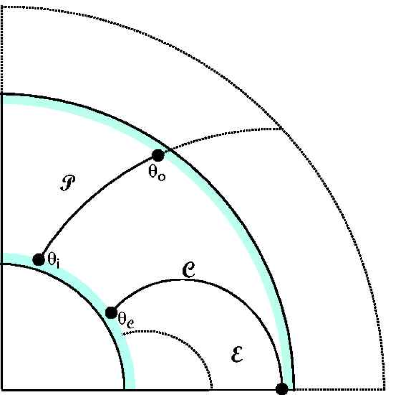
In the equatorial region $({\cal E})$, every field line (${\cal F}$) originating from the inner core in the Northern hemisphere re-enters the core at a symmetric latitude in the Southern hemisphere. In the limit of negligible diffusion, the angular velocity must be constant along (${\cal F}$) implying that the entire equatorial region must rotate with angular velocity $\Omega_{\rm in}$. The function $S$ must also be constant along (${\cal F}$), but in addition is antisymmetric with respect to the equator. The only possibility is therefore $S=0$ everywhere in $({\cal E})$.

In the polar region $({\cal P})$, field lines originating from a co-latitude $\theta_{\rm i}$ on the inner core extend out to co-latitude $\theta_{\rm o}$ on the outer boundary (see Figure 1), where

$$\frac{\sin^{2}\theta_{\rm i}}{r_{\rm i}}=\frac{\sin^{2}\theta_{\rm o}}{r_{\rm o}}\mbox{ . }$$ (18)

The field line $\cal{C}$ emerges from the inner core at co-latitude $\theta_{\cal C}$, with

$$\sin\theta_{\cal C}=\left(\frac{r_{\rm i}}{r_{\rm o}}\right)^{1/2}\mbox{ . }$$ (19)

We now consider the solutions of the problem under various types of boundary conditions for the magnetic field.

3.1 Vanishing toroidal field on the boundaries

We first consider the case where $S=r\sin\theta B_{\phi}$ is required to be zero both at the inner and the outer boundary:

$$S(r_{\rm i},\theta)=S(r_{\rm o},\theta)=0$$ (20)

These can be thought of as “insulating” boundary conditions.

3.1.1 Analytical solutions

To study the boundary layer near $r_{\rm o}$ we introduce the scaled variable

$$\xi=\frac{r_{\rm o}-r}{\delta_{\rm o}f(\theta)}\mbox{ , }$$ (21)

where the typical boundary layer thickness $\delta_{\rm o}$ and its form function $f(\theta)$ both remain to be determined. We assume (and later verify) that for low diffusivities $\delta_{\rm o}$ is very small compared with the global scales in the system ($r_{\rm i},r_{\rm o}$). Substituting this new variable in the governing equations (10) and (11), using the chain rule

$$\frac{\partial}{\partial r}\rightarrow-\frac{1}{\delta_{\rm o}f(\theta)}\frac{\partial}{\partial\xi}\mbox{ and }\frac{\partial}{\partial\theta}\rightarrow\frac{\partial}{\partial\theta}-\xi\frac{f^{\prime}(\theta)}{f(\theta)}\frac{\partial}{\partial\xi}$$ (22)

and keeping only the lowest order terms in $\delta_{\rm o}$ yields

$$\frac{\partial^{2}S}{\partial\xi^{2}} = B_{0}\frac{r_{\rm i}^{3}\delta_{\rm o}f(\theta)}{\eta r_{\rm o}}\sin^{2}\theta\cos\theta\frac{\partial\Omega}{\partial\xi}\mbox{ , }$$

$$\frac{\partial^{2}\Omega}{\partial\xi^{2}} = \frac{B_{0}}{4\pi\rho\nu}\frac{r_{\rm i}^{3}\delta_{\rm o}f(\theta)}{r_{\rm o}^{5}}\frac{\cos\theta}{\sin^{2}\theta}\frac{\partial S}{\partial\xi}\mbox{ . }$$ (23)

Combining the two equations yields

$$\frac{\partial^{3}S}{\partial\xi^{3}}=\frac{\partial S}{\partial\xi}\mbox{ and }\frac{\partial^{3}\Omega}{\partial\xi^{3}}=\frac{\partial\Omega}{\partial\xi}\mbox{ , }$$ (24)

provided we define

$$\delta_{\rm o}^{2}=\frac{4\pi\rho\nu\eta}{B^{2}_{0}}\frac{r_{\rm o}^{6}}{r_{\rm i}^{6}}\mbox{ and }f(\theta)=\frac{1}{\cos\theta}\mbox{ . }$$ (25)

The solutions to this set of equations which remain bounded as $\xi\rightarrow+\infty$ are

$$S_{\rm o}(\xi,\theta)=s_{\rm o}^{(0)}(\theta)+s_{\rm o}^{(1)}(\theta)e^{-\xi}\mbox{ , }$$

$$\Omega_{\rm o}(\xi,\theta)=\omega_{\rm o}^{(0)}(\theta)+\omega_{\rm o}^{(1)}(\theta)e^{-\xi}\mbox{ , }$$ (26)

where the index “o” denotes that this solution is only valid in the outer boundary layer. The integrating functions $s_{\rm o}^{(1)}(\theta)$ and $\omega_{\rm o}^{(1)}(\theta)$ are related to one another by the equation

$$s_{\rm o}^{(1)}(\theta)=-\left(\frac{4\pi\rho\nu}{\eta}\right)^{1/2}r_{\rm o}^{2}\sin^{2}\theta\omega_{\rm o}^{(1)}(\theta)\mbox{ . }$$ (27)

A very similar calculation can be done near $r_{\rm i}$ introducing the scaled variable

$$\zeta=\frac{r-r_{\rm i}}{\delta_{\rm i}f(\theta)}\mbox{ , }$$ (28)

with

$$\delta_{\rm i}^{2}=\frac{4\pi\rho\nu\eta}{B^{2}_{0}}\mbox{ , }$$ (29)

yielding similar governing equations (see (24)) and therefore the solutions

$$S_{\rm i}(\zeta,\theta)=s_{\rm i}^{(0)}(\theta)+s_{\rm i}^{(1)}(\theta)e^{-\zeta}\mbox{ , }$$

$$\Omega_{\rm i}(\zeta,\theta)=\omega_{\rm i}^{(0)}(\theta)+\omega_{\rm i}^{(1)}(\theta)e^{-\zeta}\mbox{ , }$$ (30)

where the index “i” denotes that this set of solutions is only valid in the inner boundary layer. The integrating functions are related to one another by

$$s_{\rm i}^{(1)}(\theta)=\left(\frac{4\pi\rho\nu}{\eta}\right)^{1/2}r_{\rm i}^{2}\sin^{2}\theta\omega_{\rm i}^{(1)}(\theta)\mbox{ . }$$ (31)

In the case of the boundary conditions selected here, the solution in the bulk of the fluid is well-approximated by neglecting any effect of dissipation. This result was formally shown by Dormy, Cardin & Jault (1998). There, $S$ and $\Omega$ are constant along magnetic field lines as discussed earlier, so we can write the bulk solution as

$$S_{\rm b}(r,\theta)=s_{\rm b}\left(A(r,\theta)\right)\mbox{ and }\Omega_{\rm b}(r,\theta)=\omega_{\rm b}\left(A(r,\theta)\right)\mbox{ . }$$ (32)

As $\xi$ and $\zeta$ respectively tend to $+\infty$, the boundary solutions must approach the bulk solution smoothly. Hence,

$$s_{\rm i}^{(0)}(\theta)=s_{\rm b}\left(A(r_{\rm i},\theta)\right)\mbox{ and }s_{\rm o}^{(0)}(\theta)=s_{\rm b}\left(A(r_{\rm o},\theta)\right)\mbox{ , }$$

$$\omega_{\rm i}^{(0)}(\theta)=\omega_{\rm b}\left(A(r_{\rm i},\theta)\right)\mbox{ and }\omega_{\rm o}^{(0)}(\theta)=\omega_{\rm b}\left(A(r_{\rm o},\theta)\right)\mbox{ . }$$ (33)

Since the co-latitudes $\theta_{\rm i}$ and $\theta_{\rm o}$ satisfy by definition $A(r_{\rm i},\theta_{\rm i})=A(r_{\rm o},\theta_{\rm o})$, the above relationships can be summarized as

$$s_{\rm i}^{(0)}(\theta_{\rm i})=s_{\rm o}^{(0)}(\theta_{\rm o})\mbox{ and }\omega_{\rm i}^{(0)}(\theta_{\rm i})=\omega_{\rm o}^{(0)}(\theta_{\rm o})\mbox{ . }$$ (34)

Finally, we apply the boundary conditions to determine the unknown integration functions uniquely. Requiring (14) and (15) implies that

$$\omega_{\rm i}^{(0)}(\theta)+\omega_{\rm i}^{(1)}(\theta)=\Omega_{\rm in}\mbox{ , }$$

$$\omega_{\rm o}^{(0)}(\theta)+\omega_{\rm o}^{(1)}(\theta)=\Omega_{\rm cz}(\theta)\mbox{ . }$$ (35)

Requiring $S=0$ on both boundaries implies

$$s_{\rm i}^{(0)}(\theta)+s_{\rm i}^{(1)}(\theta)=0\mbox{ , }$$

$$s_{\rm o}^{(0)}(\theta)+s_{\rm o}^{(1)}(\theta)=0\mbox{ . }$$ (36)

The set of eight equations contained in (27), (31), (34), (34) and (36) can be solved uniquely for the eight integration functions. Of particular interest for the following calculation is the expression for $\omega_{\rm i}^{(1)}$:

$$\omega_{\rm i}^{(1)}(\theta_{\rm i})=-\frac{r_{\rm o}^{3}}{r_{\rm o}^{3}-r_{\rm i}^{3}}\left(\Omega_{\rm cz}(\theta_{\rm o})-\Omega_{\rm in}\right)\mbox{ , }$$ (37)

where $\theta_{\rm i}$ and $\theta_{\rm o}$ are related by equation (18).

We now seek to express $\Omega_{\rm in}$ as a weighted integral over $\Omega_{\rm cz}(\theta)$. Applying (16) on the inner boundary, and using (28) and (37) yields

$$\int_{0}^{\pi/2}\sin^{3}\theta\frac{\partial\Omega_{\rm i}}{\partial r}{\rm d}\theta=-\int_{0}^{\theta_{\cal C}}\frac{\sin^{3}\theta_{\rm i}}{\delta_{\rm i}f(\theta_{\rm i})}\omega_{\rm i}^{(1)}(\theta_{\rm i}){\rm d}\theta_{\rm i}=0\mbox{ , }$$ (38)

since, in the equatorial region on the inner core ($\theta_{\rm i}>\theta_{\cal C}$), $\partial\Omega/\partial r=0$. Changing variables from $\theta_{\rm i}$ to $\theta_{\rm o}$, and using the actual expression for $f(\theta)$ transforms this equation to

$$\int_{0}^{\pi/2}\cos\theta_{\rm o}\sin^{3}\theta_{\rm o}\left[\Omega_{\rm cz}(\theta_{\rm o})-\Omega_{\rm in}\right]{\rm d}\theta_{\rm o}=0\mbox{ , }$$ (39)

which implies that

$$\Omega_{\rm in}=\Omega_{\rm eq}\left(1-\frac{a_{2}}{3}-\frac{a_{4}}{6}\right)\mbox{ . }$$ (40)

Using the helioseismically determined values for $a_{2}$ and $a_{4}$ yields

$$\Omega_{\rm in}=0.93\Omega_{\rm eq}\mbox{ . }$$ (41)

In the asymptotic limit where this expression is valid (e.g. $\delta_{\rm i}/r_{\rm i}\ll 1$) note that $\Omega_{\rm in}$ is independent of the aspect ratio $r_{\rm i}/r_{\rm o}$ of the setup, and can be shown to hold for non-homogeneous fluids as well. In fact, it only depends on the imposed differential rotation.

3.1.2 Numerical solutions

We obtained numerical solutions to the set of linearized equations (10) and (11) with boundary conditions (14), (15) and (20) using a numerical algorithm adapted from the one developed by Garaud (2001). This algorithm involves the expansion of the governing equations upon a truncated set of Chebishev functions in $\mu=\cos\theta$, and seeks the solution of the remaining set of ODEs by Newton-Raphson relaxation. The linear nature of the equations (in the variables $S$ and $\Omega$ considered) guarantees the immediate convergence of the solutions.

The analytical results presented above are asymptotically independent of the individual values selected for $B_{0}$, $\eta$ and $\rho\nu$, and depend instead only on their combination through the Hartman number $H$, which is the ratio of the geometric mean of the two diffusion times (viscous and magnetic) to the Alfvén time. From here on, we define the Hartman number of the simulation as

$$H=\frac{B_{0}r_{\rm i}}{\sqrt{4\pi\rho\nu\eta}}\mbox{ . }$$ (42)

Figure 2: Unconfined field solution for $H=4700$ and for $S=0$ on both boundaries. In our attempt to relate these simulations to the solar radiative zone, the outer solid circle marks for reference the outer edge of the Sun ($r=R_{\odot}$), and the dotted line marks the radiative–convective interface. Here, $r_{\rm o}=0.7R_{\odot}$ and $r_{\rm i}=0.35R_{\odot}$.

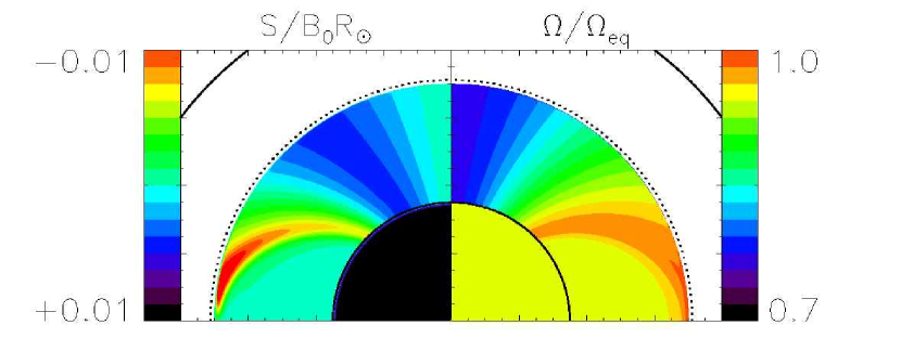
Figure 2 shows the numerical solution for a fairly large value of the Hartman number, $H=4700$. As expected, the equatorial region is indeed rotating with the same angular velocity as the core, and $S$ is zero there. In the polar regions, both $\Omega$ and $S$ are constant along poloidal magnetic field lines, except near the inner and outer boundaries, and in the vicinity of the field line $({\cal C})$. The rotation rate of the inner core is found to be $\Omega_{\rm in}=0.937\Omega_{\rm eq}$ in this simulation. This numerical solution confirms our analytical results. Moreover, as $H\rightarrow+\infty$, we find that $\Omega_{\rm in}\rightarrow 0.98\Omega_{\rm eq}$ (see Figure 7).

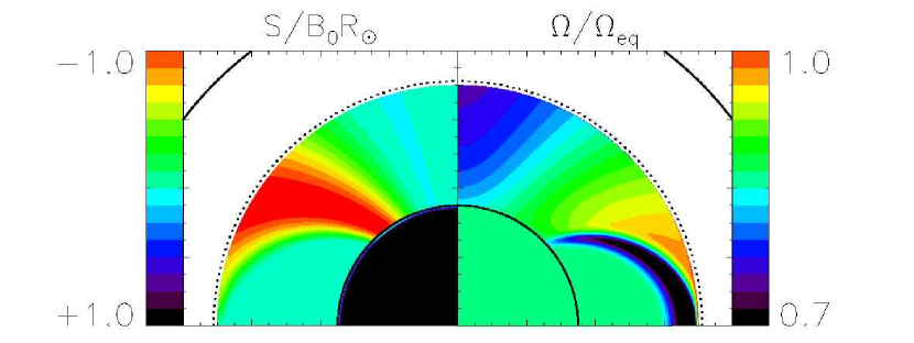
3.2 Conducting boundary conditions

We now turn to the case of “conducting boundary conditions” for the toroidal field, which are the same conditions as those used in the numerical simulations of the radiative zone dynamics performed by GG08. The material outside of the fluid shell is assumed to be infinite in extent and to have the same diffusivity as the fluid inside the shell. The toroidal field satisfies the equation

$$\nabla^{2}B_{\phi}-\frac{B_{\phi}}{r^{2}\sin^{2}\theta}=0\mbox{ , }$$ (43)

for $r>r_{\rm o}$ and $r<r_{\rm i}$, with $B_{\phi}\rightarrow 0$ as $r\rightarrow 0$ and $r\rightarrow+\infty$. The solution to this equation is smoothly matched onto the solution within the spherical shell at $r=r_{\rm i}$ and $r=r_{\rm o}$ (see GG08, for detail).

As first shown by Hollerbach (2000) the characteristics of the solution are now different from the case of insulating boundary conditions, an effect which is studied in detail by Soward & Dormy (2009). Remarkably, the bulk of the fluid is not in Ferraro isorotation. To understand the difference on a qualitative basis, note that the magnetic field is merely diffusing out of the boundaries and that the continuous generation of toroidal field by the fluid motions within the shell is only compensated by this dissipation. In other words, nothing but dissipation limits the growth of the amplitude of the field. As a result, the amplitude of $S$ is proportional to 1/$\eta$, so that the approximation ${\bf B}_{\rm p}\cdot\nabla\Omega=0$ in the bulk of the fluid is no longer valid (the diffusion term is $O(1)$ compared with the advection term). Note that ${\bf B}_{\rm p}\cdot\nabla S=0$ still holds.

Since the bulk equations are notably more difficult to solve analytically in this case (see Soward & Dormy 2009 for detail), we only provide a sample numerical solution in Figure 3. The parameters for this simulation are exactly the same as for the case shown in the previous section – only the magnetic field boundary conditions differ. The two characteristic features mentioned above are clearly illustrated in Figure 3: (1) the amplitude of the $S$ field is orders of magnitude larger than before, although $S$ is still constant on poloidal magnetic field lines; (2) the angular velocity profile deviates from Ferraro isorotation. A strong sub-rotating layer appears just interior to the field line (${\cal C}$), and the angular velocity of the inner core $\Omega_{\rm in}=0.863\Omega_{\rm eq}$ is much slower than in the previous calculation (§3.1). Finally, note that the core velocity found in this case does depend on the aspect ratio of the system. The variation of $\Omega_{\rm in}$ with $H$ is shown in Figure 7.

Figure 3: Same as Figure 2 but for conducting boundary conditions (using $(\nabla^{2}{\bf B})_{\phi}=0$ for $r>r_{\rm o}$ and $r<r_{\rm i}$). Note how the angular velocity profile is not in a state of Ferraro rotation; also note the difference in the amplitude of $S$.

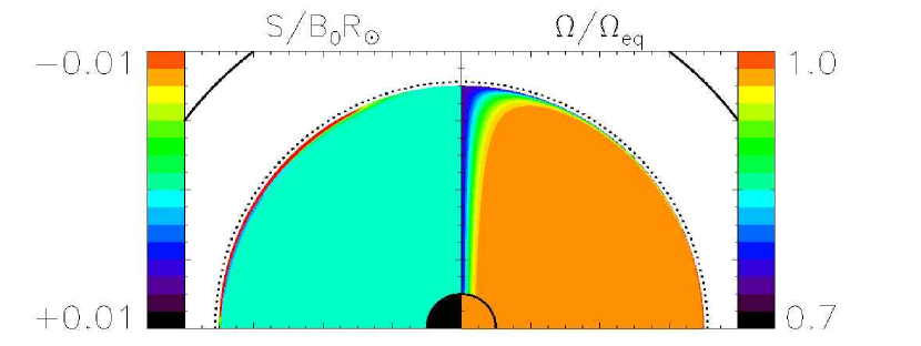
4 Solution for a confined field

In order to represent a confined magnetic field, we select the flux function $A(r,\theta)$ as in the work of Rüdiger & Kitchatinov (1997) to be

$$A(r,\theta)=B_{0}\frac{r^{2}}{2}\left(1-\frac{r}{r_{\rm o}}\right)^{q}\sin^{2}\theta\mbox{ , }$$ (44)

where $q$ is the confinement parameter, which we assume is greater or equal to one. Note that when $q=1$, $B_{r}=0$ at $r_{\rm o}$ while $B_{\theta}$ is non zero. On the other hand, for $q>1$, $B_{\theta}$ also vanishes at $r=r_{\rm o}$. Also note that the constant $B_{0}$ now defines the amplitude of the magnetic field at $r=0$ (i.e. not on the polar axis at $r=r_{\rm i}$).

We begin by considering the case of insulating boundary conditions, where $B_{\phi}=0$ at $r_{\rm i}$ and $r_{\rm o}$. Figure 4 presents a numerical solution for large Hartman number, for $q=1$. It clearly shows that the bulk of the fluid is rotating uniformly with the same angular velocity as the inner core, and that the azimuthal magnetic field is zero in the same region. This bulk solution is expected on the same symmetry grounds as the ones invoked in the equatorial region of the unconfined field case. It matches smoothly onto the applied boundary conditions at $r=r_{\rm o}$ through a boundary layer which is very thin everywhere except near the polar axis.

Figure 4: Numerical solution in the confined field case for $q=1$ and $H=1340$, using insulating boundary conditions. Here, $r_{\rm i}=0.1$ and $r_{\rm o}=0.7$. The angular velocity is constant in the bulk of the “radiative zone”, with $\Omega_{\rm in}=0.972\Omega_{\rm eq}$.

Following the method used in the case of the unconfined field configuration, we begin by rescaling the radial variable near $r_{\rm o}$ with

$$\xi=\frac{r_{\rm o}-r}{\delta_{\rm o}f(\theta)}\mbox{ , }$$ (45)

where the typical layer width $\delta_{\rm o}$ and the form function $f(\theta)$ remain to be determined. As before, we substitute this new variable for $r$ in equations (10) and (11) and keep the lowest order terms in $\delta_{\rm o}$ only, so that

$$\frac{\eta r_{\rm o}^{q-2}}{B_{0}\delta_{\rm o}^{q+1}}\xi^{1-q}\frac{\partial^{2}S}{\partial\xi^{2}}=f^{q+1}(\theta)\sin^{2}\theta\left[\frac{q\sin\theta}{2}\frac{\partial\Omega}{\partial\theta}+\left(\frac{q\sin\theta}{2}\frac{f^{\prime}(\theta)}{f(\theta)}+\cos\theta\right)\xi\frac{\partial\Omega}{\partial\xi}\right]\mbox{ , }$$

$$\frac{4\pi\rho\nu r_{\rm o}^{q+2}}{B_{0}\delta_{\rm o}^{q+1}}\xi^{1-q}\frac{\partial^{2}\Omega}{\partial\xi^{2}}=\frac{f^{q+1}(\theta)}{\sin^{2}\theta}\left[\frac{q\sin\theta}{2}\frac{\partial S}{\partial\theta}+\left(\frac{q\sin\theta}{2}\frac{f^{\prime}(\theta)}{f(\theta)}+\cos\theta\right)\xi\frac{\partial S}{\partial\xi}\right]\mbox{ . }$$ (46)

If we select

$$\delta_{\rm o}^{2q+2}=\frac{16\pi\rho\nu\eta r_{\rm o}^{2q}}{q^{2}B_{0}^{2}}\mbox{ and }f(\theta)=\frac{1}{\sin^{2/q}\theta}\mbox{ , }$$ (47)

then the variables fully separate, and the boundary layer equations become

$$\xi^{1-q}\frac{\partial^{2}}{\partial\xi^{2}}\left(\xi^{1-q}\frac{\partial^{2}S}{\partial\xi^{2}}\right)=(1-\mu^{2})^{1-1/q}\frac{\partial}{\partial\mu}\left[(1-\mu^{2})^{-1-1/q}\frac{\partial S}{\partial\mu}\right]\mbox{ , }$$

$$\xi^{1-q}\frac{\partial^{2}}{\partial\xi^{2}}\left(\xi^{1-q}\frac{\partial^{2}\Omega}{\partial\xi^{2}}\right)=(1-\mu^{2})^{-1-1/q}\frac{\partial}{\partial\mu}\left[(1-\mu^{2})^{1-1/q}\frac{\partial\Omega}{\partial\mu}\right]\mbox{ , }$$ (48)

with the introduction of the variable $\mu=\cos\theta$.

We validate our boundary layer approximation by comparing, in Figure 5, the predicted latitudinal structure of the boundary layer for $q=1$ with numerical solutions. The agreement is excellent, and similar comparisons for other values of $q$ are also in excellent agreement with (47).

Figure 5: Close up of the angular velocity profile near the outer boundary layer for $q=1$ and $H=1340$ (see Figure 4). Superimposed on this numerical solution we show the predicted boundary layer thickness $\delta_{\rm o}f(\theta)$ divided by three for the same parameter values – the two are in excellent agreement.

Even when $q=1$, solving (48) analytically is not entirely trivial. Luckily, estimating the value of the interior angular velocity does not require knowledge of the full boundary layer solution. We can obtain a first-order accurate approximation of the derivative $\partial\Omega/\partial r$ across the boundary layer with

$$\left.\frac{\partial\Omega}{\partial r}\right|_{(r_{\rm o},\theta)}\simeq\frac{\Omega_{\rm cz}(\theta)-\Omega_{\rm in}}{\delta_{\rm o}f(\theta)}\mbox{ , }$$ (49)

for large Hartman number. Applying (16) at $r_{\rm o}$ and using the approximation (49), we find that the angular velocity of the interior is determined by

$$\int_{0}^{1}(1-\mu^{2})^{1+1/q}\left[\Omega_{\rm cz}(\mu)-\Omega_{\rm in}\right]{\rm d}\mu=0\mbox{ , }$$ (50)

which implies

$$\Omega_{\rm in}=\Omega_{\rm eq}\left(1-\frac{a_{2}}{5+2/q}-\frac{3a_{4}}{(7+2/q)(5+2/q)}\right)\mbox{ . }$$ (51)

Note that as $q\rightarrow\infty$ (when the field is more and more confined), the solution recovers the purely viscous case as expected. For the helioseismically determined values of $a_{2}$ and $a_{4}$ we get

$$\Omega_{\rm in}\simeq 0.972\Omega_{\rm eq}\mbox{ for }q=1\mbox{ , }$$

$$\Omega_{\rm in}\simeq 0.966\Omega_{\rm eq}\mbox{ for }q=2\mbox{ , }$$ (52)

and so forth. To verify our analysis, we compare the asymptotic values of $\Omega_{\rm in}$ calculated in equation (51) with the numerical solutions for different values of $q$ in Fig. 6. The agreement, for high values of the Hartman number, is again excellent. Finally, it can be shown that by contrast with the unconfined field case, changing boundary conditions for the toroidal field does not yield a different asymptotic answer for $\Omega_{\rm in}$. This can be attributed to the fact that the bulk solution, and the geometry of the boundary layer, are the same regardless of the boundary conditions.

Figure 6: Calculated core velocity as a function of Hartman number. This figure compares numerical simulations and analytical predictions for $\Omega_{\rm in}/\Omega_{\rm eq}$ for two values of the confinement parameter $q$, for insulating boundary conditions. The diamonds show numerical results for $q=1$, and the plus symbols for $q=2$. The dotted line marks the analytical asymptotic limit for $q=1$ and the dashed line for $q=2$ (see equation (eq:ominconf2)). In the low Hartman number limit on the other hand, all curves converge to the value $\Omega_{\rm visc}/\Omega_{\rm eq}$ (solid line).

5 Discussion

In the two previous sections, we studied the axially symmetric, linearized dynamics of homogeneous magnetized spherical Couette flows for various geometries of the imposed poloidal field and for various types of magnetic boundary conditions. We now discuss how these simplified models may help us make sense of the dynamics of the solar radiative zone and the tachocline.

5.1 Comparison with the numerical simulations of GG08

Recently, GG08 presented a set of numerical simulations of the solar radiative zone and the tachocline based on the Gough & McIntyre model (GM98). By contrast with the toy model studied above, GG08 attempt to model the dynamics of the radiative interior as accurately as possible and solve the following system of equations

$$\overline{\rho}\tilde{{\bf u}}\cdot{\mathbf{\nabla}}\tilde{{\bf u}}+2\overline{\rho}{\bf\Omega}_{0}\times\tilde{{\bf u}}=-{\mathbf{\nabla}}\tilde{p}-\tilde{\rho}{\mathbf{\nabla}}\overline{\Phi}+{\bf j}\times{\bf B}+f_{\nu}{\mathbf{\nabla}}\cdot\Pi\mbox{ , }$$

$${\mathbf{\nabla}}\cdot(\overline{\rho}\tilde{{\bf u}})=0\mbox{ , }$$

$$\overline{\rho}\overline{T}\tilde{{\bf u}}\cdot{\mathbf{\nabla}}\overline{s}={\mathbf{\nabla}}\cdot(f_{k}\overline{k}{\mathbf{\nabla}}\tilde{T})\mbox{ , }$$

$$\frac{\tilde{p}}{\overline{p}}=\frac{\tilde{\rho}}{\overline{\rho}}+\frac{\tilde{T}}{\overline{T}}\mbox{ , }$$

$${\mathbf{\nabla}}\times(\tilde{{\bf u}}\times{\bf B})={\mathbf{\nabla}}\times(f_{\eta}\overline{\eta}{\mathbf{\nabla}}\times{\bf B})\mbox{ , }$$

$${\mathbf{\nabla}}\cdot{\bf B}=0\mbox{ , }$$ (53)

for the velocity field in the rotating frame $\tilde{{\bf u}}=(\tilde{u}_{r},\tilde{u}_{\theta},r\sin\theta\tilde{\Omega})$, for the magnetic field ${\bf B}=(B_{r},B_{\theta},B_{\phi})$ and for the density ($\tilde{\rho}$), temperature ($\tilde{T}$) and pressure ($\tilde{p}$) perturbations. In these equations, ${\bf\Omega}_{0}$ is equal to $\Omega_{\rm visc}$ (see equation (4)), the background stratification for $\bar{\rho}$ (the density), $\bar{T}$ (the temperature), $\bar{s}$ (the entropy), $\bar{\Phi}$ (the gravitational potential) and $\bar{p}$ (the pressure) are given by Model S of Christensen-Dalsgaard et al. (1996), and the diffusion coefficients $\bar{\nu}$ (for the viscosity), $\bar{\eta}$ (for the magnetic diffusivity) and $\bar{k}$ (for the thermal conductivity) are calculated according to Gough (2007) (see also GG08). Large factors $f_{\nu}$, $f_{\eta}$ and $f_{k}$ multiply these respective diffusivities to help numerical convergence. The boundary conditions used on the inner core are:

• impermeable and no-slip, with $\tilde{\Omega}=\Omega_{\rm in}-\Omega_{0}$ and where $\Omega_{\rm in}$ is deduced from (16),

• electrically conducting for the electric/magnetic field (e.g. the magnetic field satisfies ${\mathbf{\nabla}}^{2}{\bf B}=0$ in the inner core, matches on to a point dipole at $r=0$, and matches continuously to the solution in the spherical shell at $r=r_{\rm i}$),

• thermally conducting for the temperature field (e.g. $\tilde{T}$ satisfies ${\mathbf{\nabla}}^{2}\tilde{T}=0$ in the inner core, and smoothly matches on to the solution in the shell at $r=r_{\rm i}$).

The boundary conditions used on the outer boundary are:

• the velocity field matches smoothly onto an imposed velocity field

  $${\bf u}^{\rm cz}=\left(u_{r}^{\rm cz},u^{\rm cz}_{\theta},r_{\rm o}\sin\theta(\Omega_{\rm cz}-\Omega_{0})\right),$$

• electrically conducting for the electric/magnetic field (e.g. the magnetic field satisfies ${\mathbf{\nabla}}^{2}{\bf B}=0$ for $r>r_{\rm o}$, vanishes as $r\rightarrow\infty$ and smoothly matches onto the shell solution at the boundary,

• thermally conducting for the temperature field (e.g. $\tilde{T}$ satisfies ${\mathbf{\nabla}}^{2}\tilde{T}=0$ for $r>r_{\rm o}$, and smoothly matches on to the solution in the shell at $r_{\rm o}$.

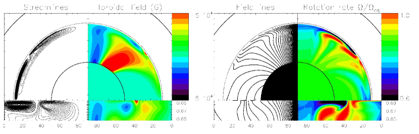
The numerical solutions of these equations and boundary conditions, as computed by GG08, exhibit many of the dynamical properties of the tachocline first discussed by GM98. In order to prevent the propagation of the convection zone shear into the interior (as illustrated in Figures 2 and 3), confining the primordial field to the radiative zone appears to be necessary. GM98 argued that large-scale meridional flows downwelling from the convection zone would naturally interact nonlinearly with the underlying field and confine it beneath the bulk of the tachocline. The convection zone flows are by the same mechanism prevented from penetrating more deeply into the radiative zone, thereby satisfying a variety of observational constraints on chemical mixing near the base of the convection zone (e.g. Elliott & Gough 1999). The tachocline would thus be a well-ventilated region, spatially separated from the magnetically-dominated interior by a very thin advection-diffusion layer. All of these features are qualitatively well-accounted for in the simulations of GG08.

However, the angular velocity of the bulk of the radiative interior in the simulations of GG08 is much lower than the observed value: $\Omega_{\rm in}\simeq 0.87\Omega_{\rm eq}$ in the limit of large Hartman number. Surprisingly, the same value is found for a fairly wide range of assumed convection zone flow amplitudes and profiles $u_{r}^{\rm cz}(\theta)$. Given that simulations robustly insist on selecting this particular interior angular velocity, can we understand it in terms of the simple dynamics studied in the toy model? Surprisingly, it appears that we can.

To see this quantitatively, Figure 7 compares the core angular velocity predictions for the stratified, nonlinear calculations of GG08 with our toy-model calculations for an open dipole in a similar experimental setup (i.e. the same aspect ratio and with conducting boundary conditions). The agreement between the two sets of simulations as a function of Hartman number is quite remarkable, in spite of the over-simplified nature of the toy model.

Figure 7: Calculated angular velocity of the core as a function of Hartman number. This figure compares the linear solutions in the toy-model (lines) and fully nonlinear numerical solutions (symbols) for two different types of boundary conditions. The conducting boundary conditions, shown in the dotted line and diamond symbols, were also used by GG08. In the limit of large Hartman number, the interior rotation rate $\Omega_{\rm in}$ tends to about $0.87\Omega_{\rm eq}$. In the second case, shown with the dashed line and triangles, we changed the lower boundary to be insulating. The asymptotic limit in both toy model and in the full numerical simulations then appears to be closer to the observations, with $\Omega_{\rm in}\rightarrow 0.93\Omega_{\rm eq}$.

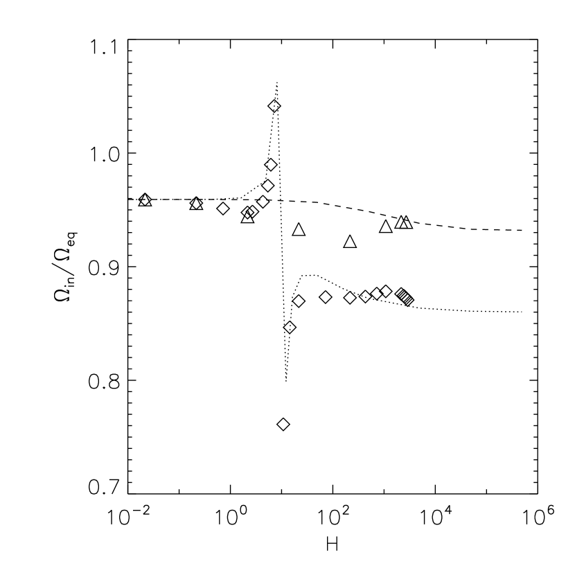
We did in fact expect the agreement to be very good for high values of the diffusivities (low values of $H$). Indeed, since the background is strongly stratified, only very slow meridional flows can penetrate into the radiative interior (see Garaud & Brummell 2008). The magnetic Reynolds number of these flows is therefore also low, and they fail to have any influence on the poloidal field. The magnetic field then naturally relaxes to its fundamental eigenmode, which is the open dipole. These combined factors together imply that the linearized problem studied in §3 should be (and is indeed found to be) a good approximation to the overall angular momentum balance of the system. It correctly predicts the asymptotic limit $H\rightarrow 0$, as well as the somewhat surprising bifurcation around $H=1$. It is also interesting to note that radial variations in $\rho$, $\nu$ and $\eta$ do not appear to affect the predictions for the interior angular velocity much. This can be formally shown in the case of insulating boundary conditions but not in the case of conducting boundary conditions. Nevertheless, it appears that the agreement approximately holds for conducting boundary conditions as well.

The good agreement between the predicted core angular velocities in the toy model and in GG08’s simulations, for low values of the diffusivities (high values of $H$), is much more surprising. The lowest-diffusivities simulations presented by GG08, which correspond to the right-most symbols in Figure 7 (see also Figure 8), have a magnetic field geometry which deviates significantly from the purely dipolar open-field configuration studied in §3. Moreover, the same simulations clearly show the existence of a region where angular-momentum transport is operated by the meridional flows rather than by the magnetic field, as predicted by GM98. Both phenomena are a natural consequence of the increasingly nonlinear nature of the interaction between the primordial field and the assumed convection zone flows as the diffusivities are lowered (equivalently, as $H$ is increased); both should by and large invalidate the applicability of the toy model. Nevertheless, even then we find that the open-dipole toy model adequately predicts the core angular velocity of the fully nonlinear numerical simulations, for the parameter values considered.

Whether this statement would continue to hold for even lower values of the diffusivities (even higher values of $H$) is a priori unlikely. As the importance of angular-momentum transport by the meridional flows increases in relation to viscous transport, we expect significant deviations away from the toy model predictions to occur. Indeed, while GG08 failed to achieve low enough diffusion parameters in their simulations to test this hypothesis, they also presented another set of simulations for artificially high convection zone flow amplitudes (see their Figure 11), in which the calculated core velocities do deviate significantly away from the toy-model predictions. Moreover, one could also expect that as the magnetic field becomes even more confined to the interior, the open-dipole configuration will lose relevance in favor of the closed-dipole configuration. Since we have shown that the closed-dipole predictions are closer to $\Omega_{\rm in}\sim 0.97\Omega_{\rm eq}$, we may expect the predicted core velocity in the full simulations to increase towards this value as the diffusivities are decreased.

5.2 Sensitivity to boundary conditions

The core velocity found in the linearized model is sensitively dependent on the assumed magnetic field boundary conditions. This was shown in §3, where changing the boundary conditions from insulating to conducting had a profound impact on the nature of the solution. In fact, it can also be shown that the same happens by changing from conducting conditions to having even just one boundary condition where $B_{\phi}=0$ (see below). But far more importantly, this sensitive dependence on boundary conditions is also found in the numerical solutions of the full set of equations (53).

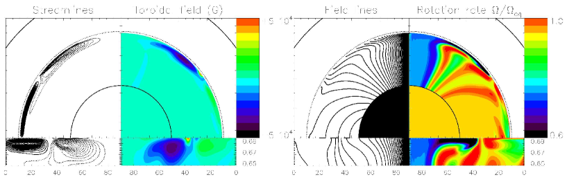
We ran a separate set of simulations for both the linearized toy model and for the full nonlinear model, where the outer boundary is again conducting but the inner core is now insulating (in the sense that $B_{\phi}=0$ at $r=r_{\rm i}$). The predictions for the core angular velocity as a function of the Hartman number are shown in Figure 7. We found that in the large-Hartman number limit, the “asymptotic” value of $\Omega_{\rm in}$ in the full nonlinear model is much closer to the observed value, $0.93\Omega_{\rm eq}$, as also predicted by the toy model. Figure 8 compares the numerical results of the full simulations with the different sets of boundary conditions with one-another. While the streamlines and the poloidal field lines (as well as the temperature and density profiles, not shown) appear to be relatively unaffected by the new boundary condition at $r_{\rm i}$, the angular velocity and toroidal field profiles are notably different. Following the trends of the toy model, the amplitude of the toroidal field is significantly lower and the rotation profile is much closer to Ferraro isorotation when at least one of the boundary conditions is not conducting.

Figure 8: Comparison between the numerical solutions of (53) with two different sets of boundary conditions on the toroidal field. Top: Conducting boundary conditions everywhere. Bottom: The top boundary is conducting while the bottom boundary is insulating. All other simulation parameters are exactly the same for the two runs: $B_{0}=7$T, $f_{\nu}=8\times 10^{8}$, $f_{\kappa}=8\times 10^{7}$ and $f_{\eta}=8\times 10^{9}$. The strip beneath each quadrant zooms into the region near the outer boundary, for $r\in[0.65,0.7]R_{\odot}$. The numbers represent latitude. In the streamlines panel, solid lines denote clockwise flows and dotted lines anti-clockwise flows.

The implications of these findings are quite important. Short of simulating the entire solar interior including the turbulent convection zone and its effect on magnetic fields, one needs to make assumptions on the nature of the radiative–convective interface. It appears that models in which the fluid shell is contained in a conducting solid of infinite extent are somewhat pathological in nature, as they allow an unphysically high magnetic field amplitude to build up thus breaking away from Ferraro isorotation (Soward & Dormy 2009). Meanwhile, insulating boundary conditions seem to be an a priori equally poor physical representation of both the inner core and of the radiative–convective interface. In reality, one may either expect other physical phenomena to limit the toroidal field amplitude within the radiative zone (e.g. magnetic instabilities), or at the very least note that the Sun is not infinite in extent, so that $B_{\phi}=0$ in the vacuum outside of $R_{\odot}$. So, as strange as it may seem, having at least one insulating boundary may actually be more physically realistic than the boundary conditions originally used by GG08.

5.3 Implications for models and observations of the solar interior

Aside from the demonstrably odd case of the conducting boundary conditions described in the previous section, all simple analytical models of the radiative zone presented so far predict an angular velocity $\Omega_{\rm in}$ close to the observations: in all cases (see Table 1), $0.908\Omega_{\rm eq}\leq\Omega_{\rm in}\leq 0.972\Omega_{\rm eq}$. Crucially, all of the estimates presented in Table 1 are independent of $\rho$, $\nu$, $\eta$, $B_{0}$ and of the aspect ratio $r_{\rm o}/r_{\rm i}$, in the asymptotic limit of large Hartman number. In addition, Garaud (2002) also studied the hydrodynamic case of spherical Couette flow between one differentially and one uniformly rotating sphere, and showed that when the gap width is of the order of the observed thickness of the tachocline, the predicted angular velocity of the interior is also, perhaps coincidentally, close to the observed value of $\Omega_{\rm rz}=0.93\Omega_{\rm eq}$.

Table 1: Summary of analytical model predictions

Model type	$\Omega_{\rm rz}/\Omega_{\rm eq}$	$\Omega_{\rm rz}/\Omega_{\rm eq}$
Viscous model	$1-\frac{a_{2}}{5}-\frac{3a_{4}}{35}$	0.959
Anisotropic viscosity	$1-\frac{3a_{2}}{7}-\frac{5a_{4}}{21}$	0.908
Open dipole field	$1-\frac{a_{2}}{3}-\frac{a_{4}}{6}$	0.930
Confined dipole field	$1-\frac{a_{2}}{5+2/q}-\frac{3a_{4}}{(5+2/q)(7+2/q)}$	0.959 - 0.972

Table 1 has a somewhat ironic property: the models which are a priori the most unphysical, or the poorest representation of the solar interior are the ones which actually seem to fare the best in terms of predicting $\Omega_{\rm in}$ close to the observed value. Indeed, recall that the open-dipole case has a non-uniformly rotating radiative zone, while the hydrodynamic spherical Couette flow (Garaud, 2002) assumes the fluid to be confined between two impermeable spherical shells.

There are several lessons to be learned from this work. As mentioned in §1, all predictions for $\Omega_{\rm in}$ necessarily involve a weighted integral over $\Omega_{\rm cz}(\theta)$. Moreover, the spherical geometry of the problem implies that the weight function is typically biased towards the equatorial regions – in other words, $\Omega_{\rm in}$ is more sensitive to $a_{2}$ than to $a_{4}$. As a result, we see that the spread in predictions for $\Omega_{\rm in}$ is relatively small, and one should neither be surprised to see many different models predicting similar values, nor that some should lie coincidentally close to the observed one.

Nevertheless, it is equally interesting to see that $\Omega_{\rm in}$ in the closed-dipole model, which is perhaps the “closest” (in relative terms) to what one may expect from the tachocline dynamics, is significantly different from the observations. This implies one of two things: either meridional flows (or perhaps anisotropic turbulent stresses) are a non-negligible contribution to angular-momentum transport in the tachocline or (if they are negligible) the true angular velocity profile near the base of the convection zone deviates significantly away from the one used here (see equation (1)). Helioseismology may be able to help distinguish between these two alternatives.

6 Conclusion

We have studied, analytically and numerically, the predicted angular velocity profile of the solar radiative zone under various model assumptions. Our overall conclusions have implications for future modeling, and implications for future observations.

In terms of modeling, we have illustrated how crucial the selection of magnetic boundary conditions can be to the calculated solution, an effect which has only recently been fully appreciated (see the detailed study by Soward & Dormy, 2009). Assuming, as previous models have done (Garaud, 2002; Brun & Zahn 2006; GG08), that the radiative zone is contained within a homogeneous conducting medium of infinite extent allows unphysically large toroidal field amplitude to build up. This case is a somewhat pathological limit, since if the toroidal field is somehow forced to be zero at a finite radius (e.g. the solar photosphere), or if other mechanisms act to limit its amplitude, then the problem does not arise. Nevertheless, how to best represent the presence of the solar convection zone remains to be determined.

In terms of observations, our various calculations have quantified the sensitivity of the angular velocity of the interior to the model assumptions: aside from a few exceptional cases which can be ruled out (see above) the predicted angular velocity lies roughly in the interval $[0.91\Omega_{\rm eq},0.97\Omega_{\rm eq}]$. Angular-momentum balance between viscous stresses and magnetic stresses for a closed-dipole suggests that $\Omega_{\rm in}\simeq 0.97\Omega_{\rm eq}$. If helioseismic observations can rule out this value entirely, then we can conclude from this study that the tachocline is the seat of additional mixing, either in the form of large-scale meridional flows (Gough & McIntyre, 1998), or in the form of small-scale turbulence. Although chemical evidence for additional mixing in the tachocline has already been put forward (Gough & McIntyre, 1998; Elliott & Gough, 1999, Rüdiger & Pipin, 2001), our work provides the first dynamical evidence to this effect.

References

- (1) Brown, T. M., Christensen-Dalsgaard, J. Dziembowsky, W. A., Goode, P., Gough, D. O. & Morrow, C. A., 1989, ApJ, 343, 526
- (2) Charbonneau, P., Christensen-Dalsgaard, J., Henning, R., Larsen, R. M., Schou, J., Thompson, M. J., & Tomczyk, S., 1999, ApJ, 527, 445
- (3) Christensen-Dalsgaard, J. & Schou, J., 1988, in Seismology of the Sun and Sun-Like Stars, ed. V. Domingo & E.J. Rolfe (ESA-SP286), p. 149
- (4) Dormy, E., Cardin, P. & Jault, D., 1998, Earth & Planetary Sci. Letters, 160, 15
- (5) Dormy, E., Jault, D. & Soward, A. M., 2002, JFM, 452, 263
- (6) Dziembowski, W. A., Goode, P. R. & Libbrecht, K. G., 1989, ApJ, 337, L53
- (7) Elliott, J. R. & Gough, D. O., 1999, ApJ, 516, 475
- (8) Ferraro, V. C. A., 1937, MNRAS, 97, 458
-
(9)
Garaud, P., 2001, PhD Thesis, available from
http://www.ams.ucsc.edu/pgaraud/Work.html - (10) Garaud, P., 2002, MNRAS, 329, 1
- (11) Garaud, P. & Brummell, N. H., 2008, ApJ, 674, 498
- (12) Garaud, P. & Garaud, J.-D., 2009, MNRAS, in press
- (13) Gilman, P.A., Morrow, C.A. & Deluca, E.E., 1989, 338, 528
- (14) Gough, D. O. & McIntyre, M. E., 1998, Nature, 394, 755
- (15) Gough, D. O., 2007. in The Solar Tachocline, pp. 3–30, eds. Hughes, D. W., Rosner, R. & Weiss, CUP.
- (16) Hollerbach, R., 2000. in Physics of rotating fluids, pp. 295–316, eds. Egbers, C. & Pfister, G. Springer.
- (17) Hollerbach, R., Canet, E. & Fournier, A., 2007, Europ. J. Mech. B, 26, 729
- (18) Miesch, M.S., 2005, LRSP, 2, 1
- (19) MacGregor, K. B. & Charbonneau, P., 1999, ApJ, 519, 911
- (20) Rüdiger, G. & Kitchatinov, L. L., 1997, Astr. Nachr. 318, 273
- (21) Rüdiger G. & Pipin, V. V., 2001, A&A, 375, 149
- (22) Soward, A.M. & Dormy, E., 2009, JFM, in prep.
- (23) Spiegel, E. A. & Zahn, J.-P., 1992, A&A, 265, 106
- (24) Tobias, S. M., Diamond, P. H. & Hughes, D. W., 2007, ApJL, 667, 113.