A Statistical Framework for Differential Privacy

Larry Wasserman^∗‡   Shuheng Zhou^{† ∗}Department of Statistics ^‡Machine Learning Department Carnegie Mellon University Pittsburgh, PA 15213 ^†Seminar für Statistik ETH Zürich, CH 8092

One goal of statistical privacy research is to construct a data release mechanism that protects individual privacy while preserving information content. An example is a random mechanism that takes an input database $X$ and outputs a random database $Z$ according to a distribution $Q_{n}(\cdot|X)$. Differential privacy is a particular privacy requirement developed by computer scientists in which $Q_{n}(\cdot|X)$ is required to be insensitive to changes in one data point in $X$. This makes it difficult to infer from $Z$ whether a given individual is in the original database $X$. We consider differential privacy from a statistical perspective. We consider several data release mechanisms that satisfy the differential privacy requirement. We show that it is useful to compare these schemes by computing the rate of convergence of distributions and densities constructed from the released data. We study a general privacy method, called the exponential mechanism, introduced by McSherry and Talwar (2007). We show that the accuracy of this method is intimately linked to the rate at which the probability that the empirical distribution concentrates in a small ball around the true distribution.

1 Introduction

One goal of data privacy research is to derive a mechanism that takes an input database $X$ and releases a transformed database $Z$ such that individual privacy is protected yet information content is preserved. This is known as disclosure limitation. In this paper we will consider various methods for producing a transformed database $Z$ and we will study the accuracy of inferences from $Z$ under various loss functions.

There are numerous approaches to this problem. The literature is vast and includes papers from computer science, statistics and other fields. The terminology also varies considerably. We will use the terms “disclosure limitation” and “privacy guarantee” interchangeably.

Disclosure limitation methods include clustering (Sweeney, 2002, Aggarwal et al., 2006), $\ell$-diversity (Machanavajjhala et al., 2006), $t$-closeness (Li et al., 2007), data swapping (Fienberg and McIntyre, 2004), matrix masking (Ting et al., 2008), cryptographic approaches (Pinkas, 2002, Feigenbaum et al., 2006), data perturbation (Evfimievski et al., 2004, Kim and Winkler, 2003, Warner, 1965, Fienberg et al., 1998) and distributed database methods (Fienberg et al., 2007, Sanil et al., 2004). Statistical references on disclosure risk and limitation include Duncan and Lambert (1986, 1989), Duncan and Pearson (1991), Reiter (2005). We refer to Reiter (2005) and Sanil et al. (2004) for further references.

One approach to defining a privacy guarantee that has received much attention in the computer science literature is known as differential privacy (Dwork et al., 2006, Dwork, 2006). There is a large body of work on this topic including, for example, Dinur and Nissim (2003), Dwork and Nissim (2004), Blum et al. (2005), Dwork et al. (2007), Nissim et al. (2007), Barak et al. (2007), McSherry and Talwar (2007), Blum et al. (2008), Kasiviswanathan et al. (2008). Blum et al. (2008) gives a machine learning approach to inference under differential privacy constraints and to some extent our results are inspired by that paper. Smith (2008) shows how to provide efficient point estimators while preserving differential privacy. He constructs estimators for parametric models with mean squared error $(1+o(1))/(nI(\theta))$ where $I(\theta)$ is the Fisher information. Machanavajjhala et al. (2008) consider privacy for histograms by sampling from the posterior distribution of the cell probabilities. We discuss Machanavajjhala et al. (2008) further in Section 4. After submitting the first draft of this paper, new work has appeared on differential privacy that is also statistical in nature, namely,  Ghosh et al. (2009), Dwork and Lei (2009), Dwork et al. (2009), Feldman et al. (2009).

The goals of this paper are to explain differential privacy in statistical language, to show how to compare different privacy mechanisms by computing the rate of convergence of distributions and densities based on the released data $Z$, and to study a general privacy method, called the exponential mechanism, due to McSherry and Talwar (2007). We show that the accuracy of this method is intimately linked to the rate at which the probability that the empirical distribution concentrates in a small ball around the true distribution. These so called “small ball probabilities” are well-studied in probability theory. To the best of our knowledge, this is the first time a connection has been made between differential privacy and small ball probabilities. We need to make two disclaimers. First, the goal of our paper is to investigate differential privacy. We will not attempt to review all approaches to privacy or to compare differential privacy with other approaches. Such an undertaking is beyond the scope of this paper. Second, we focus only on statistical properties here. We shall not concern ourselves in this paper with computational efficiency.

In Section 2 we define differential privacy and provide motivation for the definition. In Section 3 we discuss conditions that ensure that a privacy mechanism preserves information. In Section 4 we consider two histogram based methods. In Section 5 and 6, we examine another method known as the exponential mechanism. Section 7 contains a small simulation study and Section 8 contains concluding remarks. All technical proofs appear in Section 9.

1.1 Summary of Results

We consider several different data release mechanisms that satisfy differential privacy. We evaluate the utility of these mechanisms by evaluating the rate at which $d(P,P_{Z})$ goes to 0, where $P$ is the distribution of the data $X\in{\cal X}$, $P_{Z}$ is the empirical distribution of the released data $Z$, and $d$ is some distance between distributions. This gives an informative way to compare data release mechanisms. In more detail, we consider the Kolmogorov-Smirnov (KS) distance: $\sup_{x\in{\mathcal{X}}}|F(x)-\widehat{F}_{Z}(x)|$, where $F$, $\widehat{F}_{Z}$ denote the cumulative distribution function (cdf) corresponding to $P$ and the empirical distribution function corresponding to $P_{Z}$, respectively. We also consider the squared $L_{2}$ distance: $\int(p(x)-\widehat{p}_{Z})^{2}$, where $\widehat{p}_{Z}$ is a density estimator based on $Z$. Our results are summarized in the following tables, where $n$ denotes the sample size.

The first table concerns the case where the data are in $\mathbb{R}^{r}$ and the density $p$ of $P$ is Lipschitz. Also reported are the minimax rates of convergence for density estimators in KS and in squared $L_{2}$ distances. We see that the accuracy depends both on the data releasing mechanism and the distance function $d$. The results are from Sections 4 and 5 of the paper. (The exponential mechanism under $L_{2}$ distance is marked NA but is in the second table in case $r=1$. We note that the rate for KS distance for perturbed histogram is $\sqrt{\log n/n}$ for $r=1$.)

	Data Release mechanism
Distance	smoothed	perturbed	exponential	minimax
	histogram	histogram	mechanism	rate
$L_{2}$	$n^{-2/(2r+3)}$	$n^{-2/(2+r)}$	NA	$n^{-2/(2+r)}$
Kolmogorov-Smirnov	$\sqrt{\log n}\times n^{-2/(6+r)}$	$\log n\times n^{-2/(2+r)}$	$n^{-1/3}$	$n^{-1/2}$

The next table summarizes the results for the case where the dimension of $X$ is $r=1$ and the density $p$ is assumed to be in a Sobolev space of order $\gamma$. We only consider the squared $L_{2}$ distance between the true density $p$ and the estimated density $\widehat{p}_{Z}$ in this case. The results are from Section 6 of the paper.

	exponential	perturbed orthogonal	minimax rate
	mechanism	series estimator
$L_{2}$	$n^{-\gamma/(2\gamma+1)}$	$n^{-2\gamma/(2\gamma+1)}$	$n^{-2\gamma/(2\gamma+1)}$

Our results show that, in general, privacy schemes seem not to yield minimax rates. Two exceptions are perturbation methods evaluated under $L_{2}$ loss which do yield minimax rates. An open question is whether the slower than minimax rates are intrinsic to the privacy methods. It is possible, for example, that our rates are not tight. This question could be answered by establishing lower bounds on these rates. We consider this an important topic for future research.

2 Differential Privacy

Let $X_{1},\ldots,X_{n}$ be a random sample (independent and identically distributed) of size $n$ from a distribution $P$ where $X_{i}\in{\cal X}$. To be concrete, we shall assume that ${\cal X}\equiv[0,1]^{r}=[0,1]\times[0,1]\times\cdots\times[0,1]$ for some integer $r\geq 1$. Extensions to more general sample spaces are certainly possible but we focus on this sample space to avoid unnecessary technicalities. (In particular, it is difficult to extend differential privacy to unbounded domains.) Let $\mu$ denote Lebesgue measure and let $p=dP/d\mu$ if the density exists. We call $X=(X_{1},\ldots,X_{n})$ a database. Note that $X\in{\cal X}^{n}=[0,1]^{r}\times\cdots\times[0,1]^{r}$. We focus on mechanisms that take a database $X$ as input and output a sanitized database $Z=(Z_{1},\ldots,Z_{k})\in{\cal X}^{k}$ for public release. In general, $Z$ need not be the same size as $X$. For some schemes, we shall see that large $k$ can lead to low privacy and high accuracy while while small $k$ can lead to high privacy and low accuracy. We will let $k\equiv k(n)$ change with $n$. Hence, any asymptotic statements involving $n$ increasing will also allow $k$ to change as well.

A data release mechanism $Q_{n}(\cdot|X)$ is a conditional distribution for $Z=(Z_{1},\ldots,Z_{k})$ given $X$. Thus, $Q_{n}(B|X=x)$ is the probability that the output database $Z$ is in a set $B\in{\cal B}$ given that the input database is $x$, where ${\cal B}$ are the measurable subsets of ${\cal X}^{k}$. We call $Z=(Z_{1},\ldots,Z_{k})$ a sanitized database. Schematically:

$${\rm input\ database\ }X=(X_{1},\ldots,X_{n})\ \xrightarrow[\rm sanitize]{Q_{n}(Z|X)}{\rm output\ database\ }Z=(Z_{1},\ldots,Z_{k}).$$

The marginal distribution of the output database $Z$ induced by $P$ and $Q_{n}$ is $M_{n}(B)=\int Q_{n}(B|X=x)dP^{n}(x)$ where $P^{n}$ is the $n$-fold product measure of $P$.

Example 2.1.

A simple example to help the reader have a concrete example in mind is adding noise. In this case, $Z=(Z_{1},\ldots,Z_{n})$ where $Z_{i}=X_{i}+\epsilon_{i}$ and $\epsilon_{1},\ldots,\epsilon_{n}$ are mean 0 independent observations drawn from some known distribution $H$ with density $h$. Hence $Q_{n}$ has density $q_{n}(z_{1},\ldots,z_{n}|x_{1},\ldots,x_{n})=\prod_{i=1}^{n}h(z_{i}-x_{i})$.

Definition 2.2.

Given two databases $X=(X_{1},\ldots,X_{n})$ and $Y=(Y_{1},\ldots,Y_{n})$, let $\delta(X,Y)$ denote the Hamming distance between $X$ and $Y$: $\delta(X,Y)=\#\Bigl{\{}i:\ X_{i}\neq Y_{i}\Bigr{\}}$.

A general data release mechanism is the exponential mechanism (McSherry and Talwar, 2007) which is defined as follows. Let $\xi:{\cal X}^{n}\times{\cal X}^{k}:\to[0,\infty)$ be any function. Each such $\xi$ defines a different exponential mechanism. Let

$$\Delta\equiv\Delta_{n,k}=\sup_{\stackrel{{\scriptstyle x,y\in{\cal X}^{n}}}{{\delta(x,y)=1}}}\sup_{z\in{\cal X}^{k}}|\xi(x,z)-\xi(y,z)|,$$ (1)

that is, $\Delta_{n,k}$ is the maximum change to $\xi$ caused by altering a single entry in $x$. Finally, let $(Z_{1},\ldots,Z_{k})$ be a random vector drawn from the density

$$h(z|x)=\frac{\exp\left(-\frac{\alpha\xi(x,z)}{2\Delta_{n,k}}\right)}{\int_{{\cal X}^{k}}\exp\left(-\frac{\alpha\xi(x,s)}{2\Delta_{n,k}}\right)ds}$$ (2)

where $\alpha\geq 0$, $z=(z_{1},\ldots,z_{k})$ and $x=(x_{1},\ldots,x_{n})$. In this case, $Q_{n}$ has density $h(z|x)$. We’ll discuss the exponential mechanism in more detail later.

There are many definitions of privacy but in this paper we focus on the following definition due to Dwork et al. (2006) and Dwork (2006).

Definition 2.3.

Let $\alpha\geq 0$. We say that $Q_{n}$ satisfies $\alpha$-differential privacy if

$$\sup_{\stackrel{{\scriptstyle x,y\in{\cal X}^{n}}}{{\delta(x,y)=1}}}\sup_{B\in{\cal B}}\frac{Q_{n}(B|X=x)}{Q_{n}(B|X=y)}\leq e^{\alpha}$$ (3)

where ${\cal B}$ are the measurable sets on ${\cal X}^{k}$. The ratio is interpreted to be 1 whenever the numerator and denominator are both 0.

The definition of differential privacy is based on ratios of probabilities. It is crucial to measure closeness by ratios of probabilities since that protects rare cases which have small probability under $Q_{n}$. In particular, if changing one entry in the database $X$ cannot change the probability distribution $Q_{n}(\cdot|X=x)$ very much, then we can claim that a single individual cannot guess whether he is in the original database or not. The closer $e^{\alpha}$ is to 1, the stronger privacy guarantee is. Thus, one typically chooses $\alpha$ close to 0. See Dwork et al. (2006) for more discussion on these points. Indeed, suppose that two subjects each believe that one of them is in the original database. Given $Z$ and full knowledge of $P$ and $Q_{n}$ can they test who is in $X$? The answer is given in the following result. (In this result, we drop the assumption that the user does not know $Q_{n}$.)

Theorem 2.4.

Suppose that $Z$ is obtained from a data release mechanism that satisfies $\alpha$-differential privacy. Any level $\gamma$ test which is a function of $Z$, $P$ and $Q_{n}$ of $H_{0}:X_{i}=s$ versus $H_{1}:X_{i}=t$ has power bounded above by $\gamma e^{\alpha}$.

Thus, if $Q_{n}$ satisfies differential privacy then it is virtually impossible to test the hypothesis that either of the two subjects is in the database since the power of such a test is nearly equal to its level. A similar calculation shows that if one does a Bayes test between $H_{0}$ and $H_{1}$ then the Bayes factor is always between $e^{-2\alpha}$ and $e^{2\alpha}$. For more detail on the motivation for the definition as well as consequences, see Dwork et al. (2006), Dwork (2006), Ganta et al. (2008), Rastogi et al. (2009).

The following result, which is proved in McSherry and Talwar (2007) (Theorem 6), shows that the exponential mechanism always preserves differential privacy.

Theorem 2.5.

(McSherry and Talwar, 2007) The exponential mechanism satisfies the $\alpha$-differential privacy.

To conclude this section we record a few useful facts. Let $T(X,R)$ be a function of $X$ and some auxiliary random variable $R$ which is independent of $X$. After including this auxiliary random variable we define differential privacy as before. Specifically, $T(X,R)$ satisfies differential privacy if for all $B$, and all $x,x^{\prime}$ with $\delta(x,x^{\prime})=1$ we have that $\mathbb{P}(T(X,R)\in B|X=x)\leq e^{\alpha}\mathbb{P}(T(X,R)\in B|X=x^{\prime})$. The third part is Proposition 1 from Dwork et al. (2006).

Lemma 2.6.

We have the following:

1. If $T(X,R)$ satisfies differential privacy then $U=h(T(X,R))$ also satisfies differential privacy for any measurable function $h$.

2. Suppose that $g$ is a density function constructed from a random vector $T(X,R)$ that satisfies differential privacy. Let $Z=(Z_{1},\ldots,Z_{k})$ be $k$ iid draws from $g$. This defines a mechanism $Q_{n}(B|X)=\mathbb{P}(Z\in B|X)$. Then $Q_{n}$ satisfies differential privacy for any $k$.

3. (Proposition 1 from Dwork et al. (2006).) Let $f(x)$ be a function of $x=(x_{1},\ldots,x_{n})$ and define $S(f)=\sup_{x,x^{\prime}:\delta(x,x^{\prime})=1}\left\lVert f(x)-f(x^{\prime})\right\rVert_{1}$ where $\left\lVert a\right\rVert_{1}=\sum_{j}|a_{j}|$. Let $R$ have density $g(r)\propto e^{-\alpha|r|/S(f)}$. Then $T(X,R)=f(X)+R$ satisfies differential privacy.

3 Informative Mechanisms

A challenge in privacy theory is to find $Q_{n}$ that satisfies differential privacy and yet yields datasets $Z$ that preserve information. Informally, a mechanism is informative if it is possible to make precise inferences from the released data $Z_{1},\ldots,Z_{k}$. Whether or not a mechanism is informative will depend on the goals of the inference. From a statistical perspective, we would like to infer $P$ or functionals of $P$ from $Z$. Blum et al. (2008) show that the probability content of some classes of intervals can be estimated accurately while preserving privacy. Their results motivated the current paper. We will assume throughout that the user has access to the sanitized data $Z$ but not the mechanism $Q_{n}$. The question of how a data analyst can use knowledge of $Q_{n}$ to improve inferences is left to future work.

There are many ways to measure the information in $Z$. One way is through distribution functions. Let $F$ denote the cumulative distribution function (cdf) on ${\cal X}$ corresponding to $P$. Thus $F(x)=P(X\in(-\infty,x_{1}]\times\cdots\times(-\infty,x_{r}])$ where $x=(x_{1},\ldots,x_{r})$. Let $\widehat{F}\equiv\widehat{F}_{X}$ denote the empirical distribution function corresponding to $X$ and similarly let $\widehat{F}_{Z}$ denote the empirical distribution function corresponding to $Z$. Let $\rho$ denote any distance measure on distribution functions.

Definition 3.1.

$Q_{n}$ is consistent with respect to $\rho$ if $\rho(F,\widehat{F}_{Z})\stackrel{{\scriptstyle P}}{{\to}}0$. $Q_{n}$ is $\epsilon_{n}$-informative if $\rho(F,\widehat{F}_{Z})=O_{P}(\epsilon_{n})$.

An alternative to requiring $\rho(F,\widehat{F}_{Z})$ to be small is to require $\rho(\widehat{F},\widehat{F}_{Z})$ to be small. Or one could require $Q_{n}(\rho(\widehat{F},\widehat{F}_{Z})>\epsilon|X=x)$ be small for all $x$ as in Blum et al. (2008). These requirements are similar. Indeed, suppose $\rho$ satisfies the triangle inequality and that $\widehat{F}$ is consistent in the $\rho$ distance, that is, $\rho(\widehat{F},F)\stackrel{{\scriptstyle P}}{{\to}}0$. Assume further that $\rho(\widehat{F},F)=O_{P}(\epsilon_{n})$. Then $\rho(F,\widehat{F}_{Z})=O_{P}(\epsilon_{n})$ implies that

$$\rho(\widehat{F},\widehat{F}_{Z})\leq\rho(\widehat{F},F)+\rho(F,\widehat{F}_{Z})=O_{P}(\epsilon_{n});$$

Similarly, $\rho(\widehat{F},\widehat{F}_{Z})=O_{P}(\epsilon_{n})$ implies that $\rho(F,\widehat{F}_{Z})=O_{P}(\epsilon_{n})$.

Let $\mathbb{E}_{P,Q_{n}}$ denote the expectation under the joint distribution defined by $P^{n}$ and $Q_{n}$. Sometimes we write $\mathbb{E}$ when there is no ambiguity. Similarly, we use $\mathbb{P}$ to denote the marginal probability under $P^{n}$ and $Q_{n}$: $\mathbb{P}(A)=\int_{A}dQ_{n}(z_{1},\ldots,z_{k}|x_{1},\ldots,x_{n})dP(x_{1})\cdots dP(x_{n})$ for $A\in{\cal X}^{k}$.

There are many possible choices for $\rho$. We shall mainly focus on the Kolmogorov-Smirnov (KS) distance $\rho(F,G)=\sup_{x}|F(x)-G(x)|$ and the squared $L_{2}$ distance $\rho(F,G)=\int(f(x)-g(x))^{2}dx$ where $f=dF/d\mu$ and $g=dG/d\mu$. However, our results can be carried over to other distances as well.

Before proceeding let us note that we will need some assumptions on $F$ otherwise we cannot have a consistent scheme as shown in the following theorem. The following result — essentially a re-expression of a result in Blum et al. (2008) in our framework — makes this clear.

Theorem 3.2.

Suppose that $Q_{n}$ satisfies differential privacy and that $\rho(F,G)=\sup_{x}|F(x)-G(x)|$. Let $F$ be a point mass distribution. Thus $F(y)=I(y\geq x)$ for some point $x\in[0,1]$. Then $\widehat{F}_{Z}$ is inconsistent, that is, there is a $\delta>0$ such that $\liminf_{n\to\infty}P^{n}(\rho(F,\widehat{F}_{Z})>\delta)>0$.

4 Sampling From a Histogram

The goal of this section is to give two concrete, simple data release methods that achieve differential privacy. The idea is to draw a random sample from histogram. The first scheme draws observations from a smoothed histogram. The second scheme draws observations from a randomly perturbed histogram. We use the histogram for its familiarity and simplicity and because it is used in applications of differential privacy. We will see that the histogram has to be carefully constructed to ensure differential privacy. We then compare the two schemes by studying the accuracy of the inferences from the released data. We will see that the accuracy depends both on how the histogram is constructed and on what measure of accuracy we use.

Let $L>0$ be a constant and suppose that $p=dP/d\mu\in{\cal P}$ where

$${\cal P}=\Biggl{\{}p:\ |p(x)-p(y)|\leq L||x-y||\Biggr{\}}$$ (4)

is the class of Lipschitz functions. We assume throughout this section that $p\in{\cal P}$. The minimax rate of convergence for density estimators in squared $L_{2}$ distance for ${\cal P}$ is $n^{-2/(2+r)}$ (Scott, 1992).

Let $h=h_{n}$ be a binwidth such that $0<h<1$ and such that $m=1/h^{r}$ is an integer. Partition ${\cal X}$ into $m$ bins $\{B_{1},\ldots,B_{m}\}$ where each bin $B_{j}$ is a cube with sides of length $h$. Let $I(\cdot)$ denote the indicator function. Let $\widehat{f}_{m}$ denote the corresponding histogram estimator on ${\cal X}$, namely,

$$\widehat{f}_{m}(x)=\sum_{j=1}^{m}\frac{\widehat{p}_{j}}{h^{r}}I(x\in B_{j})$$

where $\widehat{p}_{j}=C_{j}/n$ and $C_{j}=\sum_{i=1}^{n}I(X_{i}\in B_{j})$ is the number of observations in $B_{j}$. Recall that $\widehat{f}_{m}$ is a consistent estimator of $p$ if $h=h_{n}\to 0$ and $nh_{n}^{r}\to\infty$. Also, the optimal choice of $m=m_{n}$ for $L_{2}$ error under ${\cal P}$ is $m_{n}\asymp n^{r/(2+r)}$, in which case $\int(p-\widehat{f}_{m})^{2}=O_{P}(n^{-2/(2+r)})$ (Scott, 1992). Here, $a_{n}\asymp b_{n}$ means that both $a_{n}/b_{n}$ and $b_{n}/a_{n}$ are bounded for large $n$.

4.1 Sampling from a Smoothed Histogram

The first method for generating released data $Z$ from a histogram while achieving differential privacy proceeds as follows. Recall that the sample space is $[0,1]^{r}$. Fix a constant $0<\delta<1$ and define the smoothed histogram

$$\widehat{f}_{m,\delta}(x)=(1-\delta)\widehat{f}_{m}(x)+\delta.$$ (5)

Theorem 4.1.

Let $Z=(Z_{1},\ldots,Z_{k})$ where $Z_{1},\ldots,Z_{k}$ are $k$ iid draws from $\widehat{f}_{m,\delta}(x)$. If

$$k\log\left(\frac{(1-\delta)m}{n\delta}+1\right)\leq\alpha$$ (6)

then $\alpha$-differential privacy holds.

Note that for $\delta\to 0$ and $\frac{m}{n\delta}\to 0$, $\log\left(\frac{(1-\delta)m}{n\delta}+1\right)=\frac{m}{n\delta}(1+o(1))\approx\frac{m}{n\delta}$. Thus (6) is approximately the same as requiring

$$\frac{mk}{\delta}\leq n\alpha.$$ (7)

Equation (7) shows an interesting tradeoff between $m$, $k$ and $\delta$. We note that sampling from the usual histogram corresponding to $\delta=0$ does not preserve differential privacy.

Now we consider how to choose $m,k,\delta$ to minimize $\mathbb{E}(\rho(F,\widehat{F}_{Z}))$ while satisfying (6). Here, $\mathbb{E}$ is the expectation under the randomness due to sampling from $P$ and due to the privacy mechanism $Q_{n}$. Thus, for any measurable function $h$,

$$\mathbb{E}(h(Z))=\int\int h(z_{1},\ldots,z_{k})dQ_{n}(z_{1},\ldots,z_{k}|x_{1},\ldots,x_{n})dP(x_{1})\cdots dP(x_{n}).$$

Now we give a result that shows how accurate the inferences are in the KS distance using the smoothed histogram sampling scheme.

Theorem 4.2.

Suppose that $Z_{1},\ldots,Z_{k}$ are drawn as described in the previous theorem. Suppose (4) holds. Let $\rho$ be the KS distance. Then choosing $m\asymp n^{r/(6+r)}$, $k\asymp m^{4/r}=n^{4/(6+r)}$ and $\delta=(mk/n\alpha)$ minimizes $\mathbb{E}\rho(F,\widehat{F}_{Z})$ subject to (6). In this case, $\mathbb{E}\rho(F,\widehat{F}_{Z})=O\left(\frac{\sqrt{\log n}}{n^{2/(6+r)}}\right).$

In this case we see that we have consistency since $\rho(F,\widehat{F}_{Z})=o_{P}(1)$ but the rate is slower than the minimax rate of convergence for density estimators in KS distance, which is $n^{-1/2}$. Now let $\widehat{q}_{j}=\#\{Z_{i}\in B_{j}\}/k$ and

$$\rho(F,\widehat{F}_{Z})=\int(p(x)-\widehat{f}_{Z}(x))^{2}dx,\;\text{where }\;\widehat{f}_{Z}(x)=h^{-r}\sum_{j=1}^{m}\widehat{q}_{j}I(x\in B_{j}).$$ (8)

Theorem 4.3.

Assume the conditions of the previous theorem. Let $\rho$ be the squared $L_{2}$ distance as defined in (8). Then choosing

$$m\asymp n^{r/(2r+3)},\ \ \ k\asymp n^{(r+2)/(2r+3)},\ \ \ \delta\asymp n^{-1/(r+3)}$$

minimizes $\mathbb{E}\rho(F,\widehat{F}_{Z})$ subject to (6). In this case, $\mathbb{E}\rho(F,\widehat{F}_{Z})=O(n^{-2/(2r+3)})$.

Again, we have consistency but the rate is slower than the minimax rate which is $n^{-2/(2+r)}$. (Scott, 1992)

4.2 Sampling From a Perturbed Histogram

The second method, which we call the sampling from a perturbed histogram, is due to Dwork et. al. (2006). Recall that $C_{j}$ is the number of observations in bin $B_{j}$. Let $D_{j}=C_{j}+\nu_{j}$ where $\nu_{1},\ldots,\nu_{m}$ are independent, identically distributed draws from a Laplace density with mean 0 and variance $8/\alpha^{2}$. Thus the density of $\nu_{j}$ is $g(\nu)=(\alpha/4)e^{-|\nu|\alpha/2}$. Dwork et. al. (2006) show that releasing $D=(D_{1},\ldots,D_{m})$ preserves differential privacy. However, our goal is to release a database $Z=(Z_{1},\ldots,Z_{k})$ rather than just a set of counts. Now define

$$\widetilde{D}_{j}=\max\{D_{j},0\}\;\text{ and }\;\widehat{q}_{j}=\widetilde{D}_{j}/\sum_{s}\widetilde{D}_{s}.$$

Since $D$ preserves differential privacy, it follows from Lemma 2.6 that $(\widehat{q}_{1},\ldots,\widehat{q}_{m})$ also preserve differential privacy; Moreover, any sample $Z=(Z_{1},\ldots,Z_{k})$ from $\widetilde{f}(x)=h^{-r}\sum_{j=1}^{m}\widehat{q}_{j}I(x\in B_{j})$ preserve differential privacy for any $k$.

Theorem 4.4.

Let $Z=(Z_{1},\ldots,Z_{k})$ be drawn from $\widetilde{f}(x)=h^{-r}\sum_{j=1}^{m}\widehat{q}_{j}I(x\in B_{j})$. Assume that there exists a constant $1\leq C<\infty$ such that $\sup_{x}p(x)=C$.
(1) Let $\rho$ be the $L_{2}$ distance and $\widehat{f}_{Z}$ be as defined in (8). Let $m\asymp n^{r/(2+r)}$ and let $k\geq n$. Then we have $\mathbb{E}\rho(F,\widehat{F}_{Z})=O(n^{-2/(2+r)})$.
(2) Let $\rho$ be the KS distance. Let $m\asymp n^{r/(2+r)}$. Then $\mathbb{E}\rho(F,\widehat{F}_{Z})=O\left(\min\left(\frac{\log n}{n^{2/(2+r)}},\sqrt{\frac{\log n}{n}}\right)\right)$.

Hence, this method achieves the minimax rate of convergence in $L_{2}$ while the first data release method does not. This suggests that the perturbation method is preferable for the $L_{2}$ distance. The perturbation method does not achieve the minimax rate of convergence in KS distance; in fact, the exponential mechanism based method achieves a better rate as we shown in Section 5 (Theorem 5.4). We examine this method numerically in Section 7.

Another approach to histograms is given by Machanavajjhala et al. (2008). They put a Dirichlet $(a_{1},\ldots,a_{m})$ prior on the cell probabilities $p_{1},\ldots,p_{m}$ where $p_{j}=\mathbb{P}(X_{i}\in B_{j})$. The corresponding posterior is Dirichlet $(a_{1}+C_{1},\ldots,a_{m}+C_{m})$. Next they draw $q=(q_{1},\ldots,q_{m})$ from the posterior and finally they sample new cell counts $D=(D_{1},\ldots,D_{m})$ from a Multinomial $(k,q)$. Thus, the distribution of $D$ given $X$ is

$$\mathbb{P}(D=d|X)=\frac{\prod_{j=1}^{m}\Gamma(d_{j}+a_{j}+C_{j})}{\Gamma(k+n+\sum_{j}a_{j})}.$$

They show that differential privacy requires $a_{j}+C_{j}\geq k/(e^{\alpha}-1)$ for all $j$. If we take $a_{1}=a_{2}=\cdots=a_{m}$ then this is similar to the first histogram-based data release method we discussed in this section. They also suggest a weakened version of differential privacy.

5 Exponential Mechanism

In this section we will consider the exponential mechanism in some detail. We’ll derive some general results about accuracy and apply the method to the mean, and to density estimation. Specifically, we will show the following for exponential mechanisms:

1. Choosing the size $k$ of the released database is delicate. Taking $k$ too large compromises privacy. Taking $k$ too small compromises accuracy.

2. The accuracy of the exponential scheme can be bounded by a simple formula. This formula has a term that measures how likely it is for a distribution based on sample size $k$, to be in a small ball around the true distribution. In probability theory, this is known as a small ball probability.

3. The formula can be applied to several examples such as the KS distance, the mean, and nonparametric density estimation using orthogonal series. In each case we can use our results to choose $k$ and to find the rate of convergence of an estimator based on the sanitized data.

In light of Theorem 3.2, we know that some assumptions are needed on $P$. We shall assume throughout this section that $P$ has a bounded density $p$; note that this is a weaker condition than (4).

Recall the exponential mechanism. We draw the vector $Z=(Z_{1},\ldots,Z_{k})$ from $h(z|x)$ where

$$h(z|x) = \frac{g_{x}(z)}{\int_{[0,1]^{k}}g_{x}(s)ds},\;\;\;\text{ where }g_{x}(z)\;=\;\exp\left(-\frac{\alpha\ \rho(\widehat{F}_{x},\widehat{F}_{z})}{2\Delta_{n,k}}\right)\;\;\text{ and }$$ (9)

$$\Delta \equiv \Delta_{n,k}\;=\;\sup_{\stackrel{{\scriptstyle x,y\in{\cal X}^{n}}}{{\delta(x,y)=1}}}\sup_{z\in{\cal X}^{k}}|\rho(\widehat{F}_{x},\widehat{F}_{z})-\rho(\widehat{F}_{y},\widehat{F}_{z})|.$$

Lemma 5.1.

For KS distance $\Delta_{n,k}\leq\frac{1}{n}$.

This framework is used in Blum et al. (2008). For the rest of this section, assume that $Z=(Z_{1},\ldots,Z_{k})$ are drawn from an exponential mechanism $Q_{n}$.

Definition 5.2.

Let $F$ denote the cumulative distribution function on $\mathcal{X}$ corresponding to $P$. Let $\widehat{G}$ denote the empirical cdf from a sample of size $k$ from $P$, and let

$$R(k,\epsilon)=P^{k}(\rho(F,\widehat{G})\leq\epsilon).$$

$R(k,\epsilon)$ is called the small ball probability associated with $\rho$.

The following theorem bounds the accuracy of the estimator from the sanitized data by a simple formula involving the small ball probability.

Theorem 5.3.

Assume that $P$ has a bounded density $p$, and that there exists $\epsilon_{n}\to 0$ such that

$$\mathbb{P}\left(\rho(F,\widehat{F}_{X})>\frac{\epsilon_{n}}{16}\right)=O\left(\frac{1}{n^{c}}\right)$$ (10)

for some $c>1$. Further suppose that $\rho$ satisfies the triangle inequality. Let $Z=(Z_{1},\ldots,Z_{k})$ be drawn from $g_{x}(z)$ given in (9). Then,

$$\mathbb{P}\left(\rho(F,\widehat{F}_{Z})>\epsilon_{n}\right)\leq\frac{(\sup_{x}p(x))^{k}\exp{\left(\frac{-3\alpha\epsilon_{n}}{16\Delta}\right)}}{R(k,\epsilon_{n}/2)}+O\left(\frac{1}{n^{c}}\right).$$ (11)

Thus, if we can choose $k=k_{n}$ in such a way that the right hand side of (11) goes to 0, then the mechanism is consistent. We now show some examples that satisfy these conditions and we show how to choose $k_{n}$.

5.1 The KS Distance

Theorem 5.4.

Suppose that $P$ has a bounded density $p$ and let $B:=\log\sup_{x}p(x)>0$. Let $Z=(Z_{1},\ldots,Z_{k})$ be drawn from $g_{x}(z)$ given in (9) with $\rho$ being the KS distance. By requiring that $k_{n}\asymp\left(\frac{3\alpha}{B}\right)^{2/3}n^{2/3}$, we have for $\epsilon_{n}=2\left(\frac{B}{3\alpha}\right)^{1/3}n^{-1/3}$, and for $\rho$ being the KS distance,

$$\rho(F,\widehat{F}_{Z})=O_{P}\left(\epsilon_{n}\right).$$ (12)

Note that $\rho(F,\widehat{F}_{Z})$ converges to 0 at a slower rate than $\rho(F,\widehat{F}_{X})$. We thus see that the rate after sanitization is $n^{-1/3}$ which is slower than the optimal rate of $n^{-1/2}$. It is an open question whether this rate can be improved.

5.2 The Mean

It is interesting to consider what happens when $\rho(F,\widehat{F}_{Z})=||\mu-\overline{Z}||^{2}$ where $\mu=\int xdP(x)$ and $\overline{Z}$ is the sample mean of $Z$. In this case $\Delta\leq r/n$. Thus, $h(u|x)\approx e^{-n||\overline{X}-\overline{Z}||^{2}/(2\alpha)}$ so, approximately, $Z_{1},\ldots,Z_{k}\sim N(\overline{X},k\alpha/n)$. Indeed, it suffices to take $k=1$ in this case since then $\overline{Z}=\overline{X}+O_{P}(1/\sqrt{n})$. Thus $\overline{Z}$ converges at the same rate as $\overline{X}$. This is not surprising: preserving a single piece of information requires a database of size $k=1$.

6 Orthogonal Series Density Estimation

In this section, we develop an exponential scheme based on density estimation and we compare it to the perturbation approach. For simplicity we take $r=1$. Let $\{1,\psi_{1},\psi_{2},\ldots,\}$ be an orthonormal basis for $L_{2}(0,1)=\{f:\ \int_{0}^{1}f^{2}(x)dx<\infty\}$ and assume that $p\in L_{2}(0,1)$. Hence

$$p(x) = 1+\sum_{j=1}^{\infty}\beta_{j}\psi_{j}(x)\;\text{ where }\;\beta_{j}=\int_{0}^{1}\psi_{j}(x)p(x)dx.$$

We assume that the basis functions are uniformly bounded so that

$$c_{0}\equiv\sup_{j}\sup_{x}|\psi_{j}(x)|<\infty.$$ (13)

Let ${\cal B}(\gamma,C)$ denote the Sobolev ellipsoid

$${\cal B}(\gamma,C)=\Biggl{\{}\beta=(\beta_{1},\beta_{2},\ldots):\ \sum_{j=1}^{\infty}\beta_{j}^{2}j^{2\gamma}\leq C^{2}\Biggr{\}}$$

where $\gamma>1/2$. Let

$${\cal P}(\gamma,C)=\Biggl{\{}p(x)=1+\sum_{j=1}^{\infty}\beta_{j}\psi_{j}(x):\ \beta\in{\cal B}(\gamma,C)\Biggr{\}}.$$

The minimax rate of convergence in $L_{2}$ norm for ${\cal P}(\gamma,C)$ is $n^{-2\gamma/(2\gamma+1)}$ (Efromovich, 1999). Thus

$$\inf_{\widehat{p}}\sup_{P\in{\cal P}(\gamma,C)}E\int(\widehat{p}(x)-p(x))^{2}dx\geq c_{1}n^{-2\gamma/(2\gamma+1)}$$

for some $c_{1}>0$. This rate is achieved by the estimator

$$\widehat{p}(x)=1+\sum_{j=1}^{m_{n}}\widehat{\beta}_{j}\psi_{j}(x)$$ (14)

where $m_{n}=n^{1/(2\gamma+1)}$ and $\widehat{\beta}_{j}=n^{-1}\sum_{i=1}^{n}\psi_{j}(X_{i}).$ See Efromovich (1999).

For a function $u\in L_{2}(0,1)$, let us define $\left\lVert u\right\rVert_{\ell_{2}}=\left(\int_{0}^{1}|u(x)|^{2}dx\right)^{1/2}$, which is a norm on $L_{2}(0,1)$. Now consider an exponential mechanism based on

$$\xi(X,Z) = \left(\int\left(\widehat{p}(x)-\widehat{p}^{*}(x)\right)^{2}dx\right)^{1/2}:=\left\lVert\widehat{p}-\widehat{p}^{*}\right\rVert_{\ell_{2}}\hskip 28.45274pt\text{where}$$ (15)

$$\widehat{p}^{*}(x) = 1+\sum_{j=1}^{m_{k}}\widehat{\beta}_{j}^{*}\psi_{j}(x),\;\text{ for}\;\;\;m_{k}=k^{\frac{1}{2\gamma+1}}\;\text{ and }\;\widehat{\beta}_{j}^{*}=k^{-1}\sum_{i=1}^{k}\psi_{j}(Z_{i}).$$ (16)

Lemma 6.1.

Under the above scheme we have $\Delta\leq\frac{2c_{0}^{2}m_{n}}{n}$ for $c_{0}$ as defined in (13). Hence,

$$g(z|x)=\exp\left(-\frac{\alpha\left\lVert\widehat{p}^{*}-\widehat{p}\right\rVert_{\ell_{2}}}{\Delta}\right)\leq\exp\left(-\frac{\alpha n\left\lVert\widehat{p}^{*}-\widehat{p}\right\rVert_{\ell_{2}}}{2c_{0}^{2}m_{n}}\right)\;\text{ almost surely.}$$ (17)

Theorem 6.2.

Let $Z=(Z_{1},\ldots,Z_{k})$ be drawn from $g_{x}(z)$ given in (17). Assume that $\gamma>1$. If we choose $k\asymp\sqrt{n}$ then

$$\rho^{2}(p,\widehat{p}^{*})=O_{P}\left(n^{-\frac{\gamma}{2\gamma+1}}\right).$$

We conclude that the sanitized estimator converges at a slower rate than the minimax rate. Now we compare this to the perturbation approach. Let $Z=(Z_{1},\ldots,Z_{k})$ be an iid sample from

$$\widehat{q}(x)=1+\sum_{j=1}^{m_{n}}(\widehat{\beta}_{j}+\nu_{j})\psi_{j}(x)$$

where $\nu_{1},\ldots,\nu_{m}$ are iid draws from a Laplace distribution with density $g(\nu)=(n\alpha/(2c_{0}m))e^{-n\alpha|\nu|/(c_{0}m)}$. Thus, i the notation of 2.6, $R=(\nu_{1},\ldots,\nu_{m})$. It follows from Lemma 2.6 that, for any $k$, this preserves differential privacy. If $\widehat{q}(x)<0$ for any $x$ then we replace $\widehat{q}$ by $\widehat{q}(x)I(\widehat{q}(x)>0)/\int\widehat{q}(s)I(\widehat{q}(s)>0)ds$ as in Hall and Murison (1993).

Theorem 6.3.

Let $Z=(Z_{1},\ldots,Z_{k})$ be drawn from $\widehat{q}$. Assume that $\gamma>1$. If we choose $k\geq n$, then

$$\rho^{2}(p,\widehat{p}_{Z})=O_{P}\left(n^{-\frac{2\gamma}{2\gamma+1}}\right)$$

where $\widehat{p}_{Z}$ is the orthogonal series density estimator based on $Z$.

Hence, again, the perturbation technique achieves the minimax rate of convergence and so appears to be superior to the exponential mechanism. We do not know if this is because the exponential mechanism is inherently less accurate, or if our bounds for the exponential mechanism are not tight enough.

7 Example

Here we consider a small simulation study to see the effect of perturbation on accuracy. We focus on the histogram perturbation method with $r=1$. We take the true density of $X$ to be a Beta(10,10) density. We considered sample sizes $n=100$ and $n=1,000$ and privacy levels $\alpha=0.1$, and $\alpha=0.01$. We take $\rho$ to be squared error distance. Figure 1 shows the results of 1,000 simulations for various numbers of bins $m$.

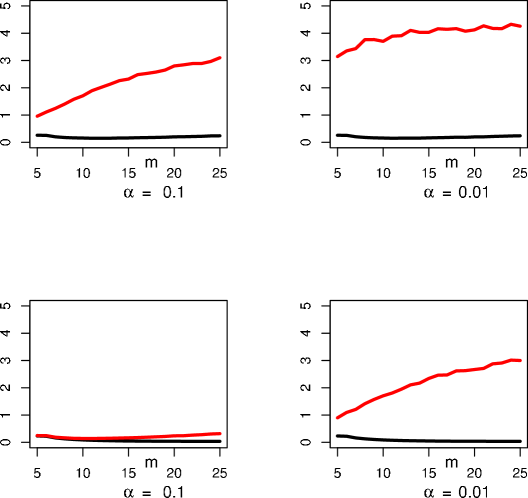
Figure 1: Top two plots $n=100$. Bottom two plots $n=1,000$. Each plot shows the mean integrated squared error of the histogram. The lower line is from the histogram based on the original data. The upper line is based on the perturbed histogram.

As expected, smaller values of $\alpha$ induce a larger information loss which manifests itself as a larger mean squared error. Despite the fact that the perturbed histogram achieves the minimax rate, the error is substantially inflated by the perturbation. This means that the constants in the risk are important, not just the rate. Also, the risk of the sanitized histograms is much more sensitive to the choice of the number of cells than the original histogram is.

We repeated the simulations with a bimodal density, namely, $p(x)$ being an equal mixture of a Beta(10,3) density and Beta(3,10) density. The results turned out to be nearly identical to those above.

8 Conclusion

Differential privacy is an important type of privacy guarantee when releasing data. Our goal has been to present the idea in statistical language and then to show that loss functions based on distributions and densities can be useful for comparing privacy mechanisms.

We have seen that sampling from a histogram leads to differential privacy as long as either the histogram is shifted away from 0 by a factor $\delta$ or if the cells are perturbed appropriately. The latter method achieves a faster rate of convergence in $L_{2}$ distance. But, the simulation showed that the risk can nonetheless be quite large. This suggests that more work is needed to get precise finite sample risk bounds. Also, the choice of the smoothing parameter (number of cells in the histogram) has a larger effect on the sanitized histogram than on the original histogram.

We also studied the exponential mechanism. Here we derived a formula for assessing the accuracy of the method. The formula involves small ball probabilities. As far as we know, the connection between differential privacy and small ball probabilities has not been observed before.

Minimaxity is desirable for any statistical procedure. We have seen that in some cases the minimax rate is achieved and in some cases it is not. We do not yet have a complete minimax theory for differential privacy and this is the focus of our current work. We close with some open questions.

1. When is it possible for $\rho(F,\widehat{F}_{Z})$ to have the same rate as $\rho(F,\widehat{F}_{X})$?

2. When adaptive minimax methods are used, such as adapting to $\gamma$ in Section 6 or when using wavelet estimation methods, is some form of adaptivity preserved after sanitization?

3. Many statistical methods involve some sort of risk minimization. A example is choosing a bandwidth by cross-validation. What is the effect of sanitization on these procedures?

4. Are there other, better methods of sanitization that preserve differential privacy?

9 Proofs

9.1 Proof of Theorem 2.4

Without loss of generality take $i=1$. Let $M_{0}(B)$ $=$ $\int Q(B|s,x_{2},\ldots,x_{n})$ $dP(x_{2},\ldots,x_{n})$ and $M_{1}(B)=\int Q(B|t,x_{2},\ldots,x_{n})dP(x_{2},\ldots,x_{n})$. By the Neyman-Pearson lemma, the highest power test is to reject $H_{0}$ when $U>u$ where $U(z)=(dM_{1}/dM_{0})(z)$ and $u$ is chosen so that $\int I(U(z)>u)dM_{0}(z)\leq\gamma$. Since $(s,x_{2},\ldots,x_{n})$ and $(t,x_{2},\ldots,x_{n})$ differ in only one coordinate, $M_{1}(B)\leq e^{\alpha}M_{0}(B)$ and so the power is $M_{1}(U>u)\leq e^{\alpha}M_{0}(U>u)\leq\gamma e^{\alpha}$.  $\;\;\scriptstyle\Box$

9.2 Proof of Lemma 2.6

For the first part simply note that $\mathbb{P}(h(T(X,R))\in B|X=x)=\mathbb{P}(T(X,R)\in h^{-1}(B)|X=x)\leq e^{\alpha}\mathbb{P}(T(X,R)\in h^{-1}(B)|X=x^{\prime})=e^{\alpha}\mathbb{P}(h(T(X,R))\in B|X=x^{\prime}).$

For the second part, let $Z=(Z_{1},\ldots,Z_{k})$ and note that $Z$ is independent of $X$ given $T(X,R)$. Let $H$ be the distribution of $T(X,R)$. Hence,

$$\mathbb{P}(Z\in B|X=x) = \int\mathbb{P}(Z\in B|X=x,T=t)dH(t|X=x)dt$$

$$= \int\mathbb{P}(Z\in B|T=t)dH(t|X=x)dt$$

$$= \int\mathbb{P}(Z\in B|T=t)\frac{dH(t|X=x)}{dH(t|X=x^{\prime})}dH(t|X=x^{\prime})$$

$$\leq e^{\alpha}\int\mathbb{P}(Z\in B|T=t)dH(t|X=x^{\prime})$$

$$= e^{\alpha}\mathbb{P}(Z\in B|X=x^{\prime}).$$

9.3 Proof of Theorem 3.2

Our proof is adapted from an argument given in Theorem 5.1. of Blum et al. (2008). Let $r=1$ so that ${\cal X}=[0,1]$. Let $P=\delta_{0}$ where $\delta_{0}$ denotes a point mass at 0. Then $P^{n}(X=X_{(0)})=1$ where $X_{(0)}\equiv\{0,\ldots,0\}$. Assume that $Q_{n}$ is consistent. Since $F(0)=1$, it follows that for any $\delta>0$, $\mathbb{P}(\widehat{F}_{Z}(0)>1-\delta)\to 1$. But since $\mathbb{P}(\cdot)=\mathbb{E}_{P}Q_{n}(\cdot|X)$ and since $P^{n}(X=X_{(0)})=1$, this implies that $Q_{n}(\widehat{F}_{Z}(0)>1-\delta|X=X_{(0)})\to 1$.

Let $v>0$ be any point in $[0,1]$ such that $Q_{n}(Z=v|X=X_{(0)})=0$. Let $X_{(1)}=\{v,0,\ldots,0\}$, $X_{(2)}=\{v,v,0,\ldots,0\}$, …, $X_{(n)}=\{v,v,\ldots,v\}$. By assumption, $Q_{n}(Z=X_{(j)}|X=X_{(0)})=0$ for all $j\geq 1$. Differential privacy implies that $Q_{n}(Z=X_{(j)}|X=X_{(1)})=0$ for all $j\geq 1$. Applying differential privacy again implies that $Q_{n}(Z=X_{(j)}|X=X_{(2)})=0$ for all $j\geq 1$. Continuing this way, we conclude that $Q_{n}(Z=X_{(j)}|X=X_{(n)})=0$ for all $j\geq 1$.

Next let $P=\delta_{v}$. Arguing as before, we know that $Q_{n}(\widehat{F}_{Z}(v)<1-\delta|X=X_{(n)})\to 0$. And since $F(v-)=0$ we also have that $Q_{n}(\widehat{F}_{Z}(v-)>\delta|X=X_{(n)})\to 0$. Here, $F(v-)=\lim_{i\to\infty}F(v_{i})$ where $v_{1}<v_{2}<\ldots$ and $v_{i}\to v$. Hence, for $j/n>1-\delta$, $Q_{n}(Z=X_{(j)}|X=X_{(n)})>0$ which is a contradiction.  $\;\;\scriptstyle\Box$

9.4 Proof of Theorem 4.1

Suppose that $X$ differs from $Y$ in at most one observation. Let $\widehat{f}$ denote the perturbed histogram $\widehat{f}_{m,\delta}$ based on $X$ and let $\widehat{g}_{m,\delta}$ denote the histogram based on $Y$, such that $X$ and $Y$ differ in one entry. We also use $\widehat{p}_{j}(X)$ and $\widehat{p}_{j}(Y)$ for cell proportions. Note that $|\widehat{p}_{j}(X)-\widehat{p}_{j}(Y)|<1/n$ by definition. It is clear that the maximum density ratio for a single draw $x_{i}$, or all $i$, occurs in one bin $B_{j}$. Now consider ${\bf x}=(x_{1},\ldots,x_{i})$ such that for all $i=1,\ldots,k$, we have $x_{i}\in B_{j}\subset[0,1]^{r}$ and the following bounds.

1. Let $\widehat{p}_{j}(Y)=0$; then in order to maximize $\widehat{f}({\bf x})/\widehat{g}({\bf x})$, we let $\widehat{p}_{j}(X)=1/n$ and obtain

   $$\frac{\widehat{f}({\bf x})}{\widehat{g}({\bf x})}=\prod_{i=1}^{k}\frac{\widehat{f}_{m,\delta}(x_{i})}{\widehat{g}_{m,\delta}(x_{i})}\leq\left(\frac{(1-\delta)m(1/n)+\delta}{\delta}\right)^{k}=\left(\frac{(1-\delta)m}{n\delta}+1\right)^{k};$$

2. Otherwise, we let $\widehat{p}_{j}(Y)\geq 1/n$, (as by definition of $\widehat{p}_{j}$, it takes $z/n$ for non-negative integers $z$) and let $\widehat{p}_{j}(X)=\widehat{p}_{j}(Y)\pm 1/n$. Now it is clear that in order to maximize the density ratio at $x$, we may need to reverse the role of $X$ and $Y$,

   $$\max\left(\frac{\widehat{g}({\bf x})}{\widehat{f}({\bf x})},\frac{\widehat{f}({\bf x})}{\widehat{g}({\bf x})}\right) \leq \max\left(\left(\frac{(1-\delta)m\widehat{p}_{j}+\delta}{(1-\delta)m(\widehat{p}_{j}-(1/n))+\delta}\right)^{k},\left(\frac{(1-\delta)m(\widehat{p}_{j}+1/n)+\delta}{(1-\delta)m\widehat{p}_{j}+\delta}\right)^{k}\right),$$

   $$\leq \max\left(\frac{(1-\delta)m(1/n)}{(1-\delta)m(\widehat{p}_{j}-(1/n))+\delta}+1\right)^{k}$$

   $$\leq \left(\frac{(1-\delta)m}{n\delta}+1\right)^{k},$$

   where the maximum is achieved when $\widehat{p}_{j}(Y)=1/n$ and $\widehat{p}_{j}(X)=0$, given a fixed set of parameters $m,n,\delta$.

Thus we have

$$\sup_{{\bf x}\in([0,1]^{r},\ldots,[0,1]^{r})}\frac{\widehat{f}({\bf x})}{\widehat{g}({\bf x})}\leq\left(\frac{(1-\delta)m}{n\delta}+1\right)^{k},$$

and the theorem holds.  $\;\;\scriptstyle\Box$

9.5 Proof of Theorem 4.2

Recall that $\widehat{F}_{Z}$ denotes the empirical distribution function corresponding to $Z=(Z_{1},\ldots,Z_{k})$, where $Z_{i}\in[0,1]^{r}$ for all $i$ are i.i.d. draws from density function $\widehat{f}_{m,\delta}(x)$ as in (5) given $X=(X_{1},\ldots,X_{n})$. Let $U$ denote the uniform cdf on $[0,1]^{r}$. Given $X=(X_{1},\ldots,X_{n})$ drawn from a distribution whose cdf is $F$, let $\widehat{f}_{m}$ denote the histogram estimator on $X$ and let $\widehat{F}_{m}(x)=\int_{0}^{x}\widehat{f}_{m}(s)ds$ and $\widehat{F}_{m,\delta}(x)=(1-\delta)\widehat{F}_{m}(x)+\delta U(x)$. Define $F_{m}(x)=\mathbb{E}(\widehat{F}_{m}(x))$ and $\bar{f}_{m}(x)=\mathbb{E}(\widehat{f}_{m}(x))$.

The Vapnik-Chervonenkis dimension of the class of sets of the form $\{(-\infty,x_{1}]\times\cdots\times(-\infty,x_{r}]$ is $r$ and so by the standard Vapnik-Chervonenkis bound, we have for $\epsilon>0$ that

$$\mathbb{P}\left(\sup_{t\in[0,1]^{r}}|\widehat{F}_{X}(t)-F(t)|>\epsilon\right) \leq 8n^{r}\exp\left\{-\frac{n\epsilon^{2}}{32}\right\}\leq\exp\left\{-\frac{n\epsilon^{2}}{64}\right\}$$ (18)

for large $n$. Hence, $\mathbb{E}\sup_{t\in[0,1]^{r}}|\widehat{F}_{X}(t)-F(t)|=O\left(\sqrt{\frac{r\log n}{n}}\right)$. Given $X$, we have $Z_{1},\ldots,Z_{k}\sim\widehat{F}_{m,\delta}$ and so $\mathbb{E}\sup_{[0,1]^{r}}|\widehat{F}_{Z}(t)-\widehat{F}_{m,\delta}(t)|=O\left(\sqrt{\frac{r\log k}{k}}\right).$ Thus,

$$\mathbb{E}\sup_{x\in[0,1]^{r}}\left\lvert\widehat{F}_{Z}(x)-F(x)\right\rvert \leq \mathbb{E}\sup_{x}|\widehat{F}_{Z}(x)-\widehat{F}_{m,\delta}(x)|+\mathbb{E}\sup_{x}|\widehat{F}_{m,\delta}(x)-F(x)|$$

$$\leq \mathbb{E}\sup_{x}|\widehat{F}_{Z}(x)-\widehat{F}_{m,\delta}(x)|+\mathbb{E}\sup_{x}|\widehat{F}_{m}(x)-F(x)|+\delta$$

$$\leq \mathbb{E}\sup_{x}|\widehat{F}_{Z}(x)-\widehat{F}_{m,\delta}(x)|+\mathbb{E}\sup_{x}|\widehat{F}_{m}(x)-F(x)|+\delta$$

$$= O\left(\sqrt{\frac{r\log k}{k}}\right)+\mathbb{E}\sup_{x}|\widehat{F}_{m}(x)-F(x)|+\delta.$$

By the triangle inequality, we have for all $x\in[0,1]^{r}$,

$$\left\lvert\widehat{F}_{m}(x)-F(x)\right\rvert\leq\left\lvert\widehat{F}_{m}(x)-F_{m}(x)\right\rvert+\left\lvert F_{m}(x)-F(x)\right\rvert,$$

and hence

$$\mathbb{E}\sup_{x\in[0,1]^{r}}\left\lvert\widehat{F}_{m}(x)-F(x)|\right\rvert \leq \mathbb{E}\sup_{x\in[0,1]^{r}}\left\lvert\widehat{F}_{m}(x)-F_{m}(x)\right\rvert+\mathbb{E}\sup_{x\in[0,1]^{r}}\left\lvert F_{m}(x)-F(x)\right\rvert$$ (19)

$$= O\left(\sqrt{\frac{r\log n}{n}}\right)+\mathbb{E}\sup_{x\in[0,1]^{r}}\left\lvert F_{m}(x)-F(x)\right\rvert$$

where the last step follows from the VC bound as in (18) for $F_{m}(x)$.

Next we bound $\sup_{x\in[0,1]^{r}}\left\lvert F_{m}(x)-F(x)\right\rvert$. Now $F(x)=P(A)$ where $A=\{(s_{1},\ldots,s_{r}):\ s_{i}\leq x_{i},i=1,\ldots,r\}$. If $x=(j_{1}h,\ldots,j_{r}h)$ for some integers $j_{1},\ldots,j_{r}$ then $F(x)-F_{m}(x)=0$. For $x$ not of this form, let $\widetilde{x}=(j_{1}h,\ldots,j_{r}h)$ where $j_{i}=\lfloor x_{i}/h\rfloor$. Let $R=\{(s_{1},\ldots,s_{r}):\ s_{i}\leq\widetilde{x}_{i},i=1,\ldots,r\}$. So

$$F(x)-F_{m}(x) = P(A)-P_{m}(A)=P(R)-P_{m}(R)+P(A\setminus R)-P_{m}(A\setminus R)$$ (20)

$$= P(A\setminus R)-P_{m}(A\setminus R)$$

where $P_{m}(B)=\int_{B}dF_{m}(u)$ and the set $A\setminus R$ intersects at most $rh/h^{r}$ number of cubes in $\{B_{1},\ldots,B_{m}\}$, given that ${\rm Vol}(A\setminus R)\leq 1-(1-h)^{r}\leq rh$. Now by the Lipschitz condition (4), we have $\sup_{x\in[0,1]^{r}}|p(x)-\bar{f}_{m}(x)|\leq Lh\sqrt{r}$ and

$$|P(A\setminus R)-P_{m}(A\setminus R)|$$

$$\leq {\rm number\ of\ cubes\ intersecting}(A\setminus R)\times{\rm maximum\ density\ discrepancy}\times{\rm volume\ of\ cube}$$

$$\leq (rh/h^{r})\cdot(Lh\sqrt{r})\cdot h^{r}\leq Lr^{3/2}m^{-2/r}.$$ (21)

Thus we have by (19), (20) and (21)

$$\mathbb{E}\sup_{x}|\widehat{F}_{m}(x)-F(x)|=O\left(\sqrt{\frac{r\log n}{n}}\right)+Lr^{3/2}m^{-2/r}.$$ (22)

Hence,

$$\mathbb{E}\sup_{x}|\widehat{F}_{Z}(x)-F(x)|=O\left(\sqrt{\frac{r\log k}{k}}\right)+O\left(\sqrt{\frac{r\log n}{n}}\right)+Lr^{3/2}m^{-2/r}+\delta.$$

Set $m\asymp n^{r/(6+r)}$, $k\asymp m^{4/r}=n^{4/(6+r)}$ and $\delta=(mk/n\alpha)$ we get for all $n$ large enough, $\mathbb{E}\sup_{x}|\widehat{F}_{Z}(x)-F(x)|=O\left(\frac{\sqrt{\log n}}{n^{2/(6+r)}}\right).$  $\;\;\scriptstyle\Box$

9.6 Proof of Theorem 4.3

Let $\widehat{f}_{Z}$ be the histogram based on $Z$ as in (8). Then

$$(\widehat{f}_{Z}(u)-p(u))^{2}\preceq(1-\delta)^{2}(p(u)-\widehat{f}_{m}(u))^{2}+\delta^{2}(p(u)-1)^{2}+(\widehat{f}_{m,\delta}(u)-\widehat{f}_{Z})^{2}$$

where $\preceq$ means less than, up to constants. Hence,

$$\mathbb{E}\int(\widehat{f}_{Z}(u)-p(u))^{2}du\preceq R_{m}+\delta^{2}+\mathbb{E}\int(\widehat{f}_{m,\delta}(u)-\widehat{f}_{Z}(u))^{2}du$$

where $R_{m}$ is the usual $L_{2}$ risk of a histogram under the Lipschitz condition (4), namely, $m^{-2/r}+m/n$. Conditional on $X$, $\widehat{f}_{Z}$ is an unbiased estimate of $\widehat{f}_{m}$ with integrated variance $m/k$. So,

$$\mathbb{E}\int(\widehat{f}_{Z}(u)-p(u))^{2}du\preceq m^{-2/r}+\frac{m}{n}+\delta^{2}+\frac{m}{k}.$$

Minimizing this, subject to (6) yields

$$m\asymp n^{r/(2r+3)},k\asymp n^{(r+2)/(2r+3)},\delta\asymp n^{-1/(2r+3)}$$

which yields $\mathbb{E}\int(\widehat{f}_{Z}(u)-p(u))^{2}du=O(n^{-2/(2r+3)}).$  $\;\;\scriptstyle\Box$

9.7 Proof of Theorem 4.4

(1) Note that $p-\widehat{f}_{Z}=p-\widetilde{f}+\widetilde{f}-\widehat{f}_{Z}=p-\widetilde{f}+O_{P}\left(\frac{m}{k}\right).$ When $k\geq n$, the latter error is lower order than the other terms and may be ignored. Now,

$$p(x)-\widetilde{f}(x)=p(x)-\widehat{f}_{m}(x)+\widehat{f}_{m}(x)-\widetilde{f}(x).$$

Thus

$$\int(p(x)-\widetilde{f}(x))^{2}dx\preceq\int(p(x)-\widehat{f}_{m}(x))^{2}dx+\int(\widehat{f}_{m}(x)-\widetilde{f}(x))^{2}dx.$$

The expected value of the first term is the usual risk, namely, $O(m^{-2/r}+m/n)$.

For the second term, we proceed as follows. Let $\widehat{p}_{j}=C_{j}/n$ and

$$\widehat{q}_{j}=\frac{(C_{j}+\nu_{j})_{+}}{\sum_{s=1}^{m}(C_{s}+\nu_{s})_{+}}.$$

We claim that

$$\max_{j}|\widehat{q}_{j}-\widehat{p}_{j}|=O\left(\frac{\log m}{n}\right)$$

almost surely, for all large $n$. We have

$$\widehat{q}_{j}=\frac{(C_{j}+\nu_{j})_{+}}{n}\left(\frac{n}{\sum_{s=1}^{m}(C_{s}+\nu_{s})_{+}}\right)=\frac{(C_{j}+\nu_{j})_{+}}{n}\frac{1}{R_{n}}$$

where $R_{n}=(\sum_{s=1}^{m}(C_{s}+\nu_{s})_{+})/n$. Now

$$\widehat{p}_{j}-\frac{|\nu_{j}|}{n}\leq\widehat{p}_{j}+\frac{\nu_{j}}{n}=\frac{(C_{j}+\nu_{j})}{n}\leq\frac{(C_{j}+\nu_{j})_{+}}{n}\leq\widehat{p}_{j}+\frac{|\nu_{j}|}{n}.$$

Therefore,

$$\left|\frac{(C_{j}+\nu_{j})_{+}}{n}-\widehat{p}_{j}\right|\leq\frac{|\nu_{j}|}{n}\leq\frac{M}{n}$$

where $M=\max\{|\nu_{1}|,\ldots,|\nu_{m}|\}$. Let $A>0$. The density for $\nu_{j}$ has the form $f(\nu)=(\beta/2)e^{-\beta|\nu|}$. So,

$$\mathbb{P}(M>A\log m)\leq m\mathbb{P}(|\nu_{j}|>A\log m)=\beta m\int_{A\log m}^{\infty}e^{-\beta|\nu|}d\nu=\frac{1}{m^{A\beta-1}}.$$

By choosing $A$ large enough we have that $M<A\log m$ a.s. for large $n$, by the Borel-Cantelli lemma. Therefore,

$$\left|\frac{(C_{j}+\nu_{j})_{+}}{n}-\widehat{p}_{j}\right|\leq\frac{\log m}{n}$$

Now we bound $R_{n}$. We have

$$1-\frac{\sum_{s}|\nu_{s}|}{n}\leq 1+\frac{\sum_{s}\nu_{s}}{n}\leq R_{n}=\frac{\sum_{s=1}^{m}(C_{s}+\nu_{s})_{+}}{n}\leq 1+\frac{\sum_{s}|\nu_{s}|}{n}$$

so that

$$|R_{n}-1|\leq\frac{\sum_{s}|\nu_{s}|}{n}\leq\frac{Mm}{n}=O\left(\frac{m\log m}{n}\right)\ \ \ a.s.$$

Therefore, $1/R_{n}=(1+O(m\log m/n))$ and thus

$$\widehat{q}_{j} = \left(\widehat{p}_{j}+O\left(\frac{\log m}{n}\right)\right)\ \left(1+O\left(\frac{m\log m}{n}\right)\right)$$

$$= \widehat{p}_{j}+\widehat{p}_{j}\ O\left(\frac{m\log m}{n}\right)+O\left(\frac{\log m}{n}\right)+O\left(\frac{m(\log m)^{2}}{n^{2}}\right).$$

Next we claim that $\widehat{p}_{j}=O(1/m)$ a.s. To see this, note that $p_{j}\leq C/m$, by definition of $C$: $1\leq C=\sup_{x}p(x)<\infty$. Hence, by Bernstein’s inequality,

$$\mathbb{P}\left(\widehat{p}_{j}>\frac{2C}{m}\right) = \mathbb{P}\left(\widehat{p}_{j}-p_{j}>\frac{2C}{m}-p_{j}\right)\leq\exp\left\{-\frac{1}{2}\frac{n((2C/m)-p_{j})^{2}}{p_{j}+\frac{1}{3}((2C/m)-p_{j})}\right\}$$

$$\leq \exp\left\{-\frac{1}{2}\frac{nC^{2}/m^{2}}{(4C/3m)}\right\}=e^{-3nC/(8m)}\leq\frac{1}{n^{2}}$$

for all $n\geq 16m\log n/3C$; Thus $\widehat{p}_{j}=O(1/m)$ a.s. for all large $n$. Thus, $\widehat{q}_{j}-\widehat{p}_{j}=O(\log m/n)$ almost surely for all large $n$. Hence,

$$\mathbb{E}\int(\widehat{f}_{m}(x)-\widetilde{f}(x))^{2}dx=O\left(\frac{m\log m}{n}\right)^{2}.$$

So the risk is

$$O\left(m^{-2/r}+\frac{m}{n}+\left(\frac{m\log m}{n}\right)^{2}\right)=O\left(m^{-2/r}+\frac{m}{n}\right),$$

for $n\geq m\log^{2}m$. This is the usual risk. Hence, we can choose $m\asymp n^{r/(2+r)}$ to achieve risk $n^{-2/(2+r)}$ for all $n$ large enough.

(2) Let $\widehat{F}_{m}$ be the cdf based on the original histogram and let $\widetilde{F}_{m}$ be the cdf based on the perturbed histogram. We have

$$\mathbb{E}\sup_{x}|F(x)-\widehat{F}_{Z}(x)| \leq \mathbb{E}\sup_{x}|F(x)-\widehat{F}_{m}(x)|+\mathbb{E}\sup_{x}|\widehat{F}_{m}(x)-\widetilde{F}_{m}(x)|+\mathbb{E}\sup_{x}|\widetilde{F}_{m}(x)-\widehat{F}_{Z}(x)|$$

$$\leq \mathbb{E}\sup_{x}|F(x)-\widehat{F}_{m}(x)|+\mathbb{E}\sup_{x}|\widehat{F}_{m}(x)-\widetilde{F}_{m}(x)|+O\left(\sqrt{\frac{r\log k}{k}}\right).$$

Since we may take $k$ as large as we like, we can make the last term arbitrarily small. From (22),

$$\mathbb{E}\sup_{x}|F(x)-\widehat{F}_{m}(x)|=O\left(\sqrt{\frac{r\log n}{n}}\right)+Lr^{3/2}m^{-2/r}.$$

Let $\widehat{f}(x)=h^{-r}\sum_{j=1}^{m}\widehat{p}_{j}I(x\in B_{j})$ and Let $\widetilde{f}(x)=h^{-r}\sum_{j=1}^{m}\widehat{q}_{j}I(x\in B_{j})$. Let $x^{\prime}=(u_{1}h,\ldots,u_{r}h)$ where $u_{i}=\lceil x_{i}/h\rceil,\forall i=1,\ldots,r$. Recall that $B_{1},\ldots,B_{m}$ are the $m$ bins of $\mathcal{X}$ with sides of length of $h$. Let $B_{x}$ denote the cube with the left-most corner being $0$ and the right-most corner being $x$. Then for all $x$, we have

$$\left\lvert\widehat{F}_{m}(x)-\widetilde{F}_{m}(x)\right\rvert = \left\lvert\int_{0}^{x}\widehat{f}(s)-\widetilde{f}(s)ds\right\rvert\leq\int_{0}^{x}\left\lvert\widehat{f}(s)-\widetilde{f}(s)\right\rvert ds$$

$$\leq \int_{0}^{x^{\prime}}\left\lvert\widehat{f}(s)-\widetilde{f}(s)\right\rvert ds$$

$$= \sum_{\ell:B_{\ell}\subseteq B_{x^{\prime}}}|\widehat{p}_{\ell}-\widehat{q}_{\ell}|\leq\sum_{\ell=1}^{m}|\widehat{p}_{\ell}-\widehat{q}_{\ell}|$$

where we use the fact that there are at most $m$ cubes. Hence,

$$\mathbb{E}\sup_{x\in[0,1]^{r}}|\widehat{F}_{m}(x)-\widetilde{F}_{m}(x)| \leq \frac{m\log m}{n}$$

where we use the fact that $\max_{j}|\widehat{p}_{j}-\widehat{q}_{j}|=O(\log m/n)$ a.s. So,

$$\mathbb{E}\sup_{x}|F(x)-\widehat{F}_{Z}(x)|=O\left(\sqrt{\frac{r\log n}{n}}\right)+Lr^{3/2}m^{-2/r}+O\left(\frac{m\log m}{n}\right).$$

Setting $m\asymp n^{r/(2+r)}$ yields

$$\mathbb{E}\sup_{x}|F(x)-\widehat{F}_{Z}(x)|=O\left(\min\left(\frac{\log n}{n^{2/(2+r)}},\sqrt{\frac{\log n}{n}}\right)\right)$$

Hence for $r=1$, the rate is $O\left(\sqrt{\frac{\log n}{n}}\right)$. For $r\geq 2$, the rate is dominated by the first term inside $O()$, and hence the rate is $O\left(\log n\times n^{-2/(2+r)}\right)$.  $\;\;\scriptstyle\Box$

9.8 Proof of Theorem 5.3

Let $B_{\epsilon}=\Bigl{\{}u=(u_{1},\ldots,u_{k}):\ \rho(F,\widehat{F}_{u})\leq\epsilon\Bigr{\}}$ where $\widehat{F}_{u}$ is the empirical distribution based on $u=(u_{1},\ldots,u_{k})\in{\cal X}^{k}$. Also, let $A_{n}=\{\rho(\widehat{F}_{X},F)\leq\epsilon_{n}/16\}$. For notational simplicity set $\Delta=\Delta_{n,k}$. Then

$$\mathbb{P}\left(\rho(F,\widehat{F}_{Z})>\epsilon_{n}\right) = \mathbb{P}\left(\rho(F,\widehat{F}_{Z})>\epsilon_{n},A_{n}\right)+\mathbb{P}\left(\rho(F,\widehat{F}_{Z})>\epsilon_{n},A_{n}^{c}\right)$$ (23)

$$\leq \mathbb{P}\left(\rho(F,\widehat{F}_{Z})>\epsilon_{n},A_{n}\right)+\mathbb{P}\left(A_{n}^{c}\right)$$

$$= \mathbb{P}\left(\rho(F,\widehat{F}_{Z})>\epsilon_{n},A_{n}\right)+O\left(\frac{1}{n^{c}}\right).$$

By the triangle inequality $\rho(\widehat{F}_{u},\widehat{F}_{X})\geq\rho(\widehat{F}_{u},F)-\rho(\widehat{F}_{X},F)$. Then,

$$\int_{B_{\epsilon}^{c}}g_{x}(u)du = \int_{B_{\epsilon}^{c}}\exp{\left(\frac{-\alpha\rho(\widehat{F}_{X},\widehat{F}_{u})}{2\Delta}\right)}du$$

$$\leq \int_{B_{\epsilon}^{c}}\exp{\left(\frac{-\alpha(\rho(\widehat{F}_{u},F)-\rho(\widehat{F}_{X},F))}{2\Delta}\right)}du$$

$$= \exp{\left(\frac{\alpha\rho(\widehat{F}_{X},F)}{2\Delta}\right)}\int_{B_{\epsilon}^{c}}\exp{\left(\frac{-\alpha\rho(\widehat{F}_{u},F)}{2\Delta}\right)}du$$

$$\leq \exp{\left(\frac{\alpha\rho(\widehat{F}_{X},F)}{2\Delta}\right)}\exp{\left(\frac{-\alpha\epsilon}{2\Delta}\right)}\int_{B_{\epsilon}^{c}}du$$

$$\leq \exp{\left(\frac{\alpha\rho(\widehat{F}_{X},F)}{2\Delta}\right)}\exp{\left(\frac{-\alpha\epsilon}{2\Delta}\right)}.$$

By the triangle inequality, we also have $\rho(\widehat{F}_{u},\widehat{F}_{X})\leq\rho(\widehat{F}_{u},F)+\rho(\widehat{F}_{X},F)$ and

$$\int g_{x}(u)du \geq \int_{B_{\epsilon/2}}g_{x}(u)du=\int_{B_{\epsilon/2}}\exp{\left(\frac{-\alpha\rho(\widehat{F}_{X},\widehat{F}_{u})}{2\Delta}\right)}du$$

$$\geq \exp{\left(\frac{-\alpha\rho(\widehat{F}_{X},F)}{2\Delta}\right)}\int_{B_{\epsilon/2}}\exp{\left(\frac{-\alpha\rho(F,\widehat{F}_{u})}{2\Delta}\right)}du$$

$$\geq \exp{\left(\frac{-\alpha\rho(\widehat{F}_{X},F)}{2\Delta}\right)}\exp{\left(\frac{-\alpha\epsilon}{4\Delta}\right)}\int_{B_{\epsilon/2}}du$$

$$= \exp{\left(\frac{-2\alpha\rho(\widehat{F}_{X},F)-\alpha\epsilon}{4\Delta}\right)}\int_{B_{\epsilon/2}}\frac{p(u_{1})\cdots p(u_{k})}{p(u_{1})\cdots p(u_{k})}du$$

$$\geq \frac{\exp{\left(\frac{-2\alpha\rho(\widehat{F}_{X},F)-\alpha\epsilon}{4\Delta}\right)}}{(\sup_{x}p(x))^{k}}\mathbb{P}\left(\rho(F,\widehat{G})\leq\epsilon/2\right)$$

where $\widehat{G}$ is the empirical cdf from a sample of size $k$ drawn from $P$. Thus we have

$$\int_{B_{\epsilon}^{c}}h(u|x)du \leq \frac{{(\sup_{x}p(x))^{k}}\exp{\left(\frac{\alpha\rho(\widehat{F}_{X},F)}{\Delta}\right)}\exp{\left(\frac{-\alpha\epsilon}{4\Delta}\right)}}{\mathbb{P}\left(\rho(F,\widehat{G})\leq\epsilon/2\right)}.$$

Thus, from (23),

$$\mathbb{P}\left(\rho(F,\widehat{F}_{Z})>\epsilon\right) \leq \mathbb{P}\left(\rho(\widehat{F}_{X},F)\geq\frac{\epsilon}{16}\right)+\frac{{(\sup_{x}p(x))^{k}}\exp{\left(\frac{-3\alpha\epsilon}{16\Delta}\right)}}{\mathbb{P}\left(\rho(F,\widehat{G})\leq\epsilon/2\right)}$$

$$= \frac{{(\sup_{x}p(x))^{k}}\exp{\left(\frac{-3\alpha\epsilon}{16\Delta}\right)}}{\mathbb{P}\left(\rho(F,\widehat{G})\leq\epsilon/2\right)}+O\left(\frac{1}{n^{c}}\right).$$

Thus the theorem holds.  $\;\;\scriptstyle\Box$

9.9 Proof of Lemma 5.1

Proof of Lemma 5.1. We start with KS, By the triangle inequality, we have for all $z\in{\mathcal{X}}^{k}$ and for all $x,y\in{\mathcal{X}}^{n}$,

$$\left\lvert\rho(\widehat{F}_{x},\widehat{F}_{z})-\rho(\widehat{F}_{y},\widehat{F}_{z})\right\rvert \leq \rho(\widehat{F}_{x},\widehat{F}_{y}).$$

Notice that changing one entry in $x$ will change $\widehat{F}_{x}(t)$ by at most $\frac{1}{n}$ at any $t$ by definition, that is,

$$\sup_{t\in[0,1]^{r}}|\widehat{F}_{x}(t)-\widehat{F}_{y}(t)| = \frac{1}{n}.$$

Thus the conclusion holds for the KS-distance.  $\;\;\scriptstyle\Box$

9.10 Proof of Theorem 5.4

We need the following small ball result; see Li and Shao (2001).

Theorem 9.1.

Let $r\geq 3$, and $\{X_{t},t\in[0,1]^{r}\}$ be the Brownian sheet. Then there exists $0<C_{r}<\infty$ such that for all $0<\epsilon\leq 1$,

$$\log\mathbb{P}\left(\sup_{t\in[0,1]^{r}}|X_{t}|\leq\epsilon\right)\geq-C_{r}\epsilon^{-2}\log^{2r-1}(1/\epsilon)$$

where $C_{r}$ depends only on $r$. The same bound holds for a Brownian bridge.

Proof of theorem 5.4.   The Vapnik-Chervonenkis dimension of the class of sets of the form $\{(-\infty,x_{1}]\times\cdots\times(-\infty,x_{r}]$ is $r$ and so by the standard Vapnik-Chervonenkis bound, we have for $\epsilon_{n},k_{n}$ as specified in the theorem statement,

$$\mathbb{P}\left(\sup_{[0,1]^{r}}|\widehat{F}_{X}(t)-F(t)|>\frac{\epsilon_{n}}{16}\right) \leq 8n^{r}\exp\left\{-\frac{n(\epsilon_{n}/16)^{2}}{32}\right\}$$ (24)

$$\leq 8\exp\left\{-c_{5}\left(\frac{B}{3\alpha}\right)^{2/3}n^{1/3}+r\log n\right\}$$

$$= 8\exp\left\{-c_{6}\sqrt{k_{n}}\left(\frac{B}{3\alpha}\right)+c_{7}r\log k_{n}\right\}$$

$$= 8\exp\left\{-C_{2}\sqrt{k_{n}}\left(\frac{B}{3\alpha}\right)\right\}$$

for some constants $c_{5},c_{6},c_{7},C_{2}>0$ for $n$ large enough. Thus (10) holds. Now we compute the small ball probability. Note that $\sqrt{k}(\widehat{F}_{k}-F)$ converges to a Brownian bridge $B_{k}$ on $[0,1]^{r}$. More precisely, from Csörgő and Révész (1975) there exist a sequence of Brownian bridges $B_{k}$ such that

$$\sup_{t}|\sqrt{k}(\widehat{F}_{k}-F)(t)-B_{k}(t)|=O\left(\frac{(\log k)^{3/2}}{k^{\gamma}}\right)\ \ \ \ \text{ a.s. }$$ (25)

where $\gamma=1/(2(r+1))$. It is clear that the RHS of (25) is $o(1)$ a.s. given a fixed $r$. Hence we have for $k=k_{n}$ and $\epsilon_{n}$ as chosen in the theorem statement, and for all $\epsilon\geq\epsilon_{n}$, it holds that

$$\log\mathbb{P}(\sup_{t}|\widehat{F}_{Z}(t)-F(t)|\leq\epsilon/2) = \log\mathbb{P}(\sup_{t}\sqrt{k}|\widehat{F}_{Z}(t)-F(t)|\leq\sqrt{k}\epsilon/2)$$ (26)

$$\geq \log\mathbb{P}\left(\sup_{t}|B_{k}(t)|\leq\sqrt{k}\epsilon-O\left(k^{-\gamma}(\log k)^{3/2}\right)\right)$$

$$\geq \log\mathbb{P}\left(\sup_{t}|B_{k}(t)|\leq\frac{\sqrt{k}\epsilon}{4}\right)$$ (27)

for all large $n$, where (26) follows from (25) and (27) holds given that $\sqrt{k}\epsilon\geq\sqrt{k_{n}}\epsilon_{n}\geq c$ for some constant $c>1/2$ due to our choice of $k_{n}$ and $\epsilon_{n}$. Also, $\Delta\leq 1/n$ for KS distance. Hence, by Theorem 5.3 and (24), we have for $B=\log\sup_{x}p(x)>0$,

$$\mathbb{P}\left(\rho(F,\widehat{F}_{Z})>\epsilon_{n}\right)$$ (28)

$$\leq C_{0}\exp\left\{-n\left(\frac{3\alpha\epsilon_{n}}{16}-\frac{Bk_{n}}{n}-\frac{C_{1}|\log(\sqrt{k_{n}}\epsilon_{n}/4)|^{2r-1}}{nk_{n}\epsilon_{n}^{2}}\right)\right\}+8\exp\left\{-C_{2}\frac{B\sqrt{k_{n}}}{3\alpha}\right\}$$

$$\leq C_{0}\exp(-C_{3}Bk_{n}/2)+8\exp\left\{-C_{2}\left(\frac{B}{3\alpha}\right)\sqrt{k_{n}}\right\}\to 0$$

for some constants $C_{0},C_{1},C_{2}$ and $C_{3}$, where (28) holds when we take w.l.o.g. $k_{n}=\frac{1}{16}\left(\frac{3\alpha}{B}\right)^{2/3}n^{2/3}$ and $\epsilon_{n}\geq 2\left(\frac{B}{3\alpha}\right)^{1/3}n^{-1/3}$, given that $\epsilon_{n}\geq 2\left(\frac{B}{3\alpha}\right)^{1/3}n^{-1/3}=\frac{32k_{n}B}{3n\alpha}$ and hence $\frac{3\alpha\epsilon_{n}}{16}\geq\frac{2Bk_{n}}{n}$. Thus the result follows.  $\;\;\scriptstyle\Box$

Remark 9.2.

The constants taken in the proof are arbitrary; indeed, when we take $k_{n}=C_{4}\left(\frac{3\alpha}{B}\right)^{2/3}n^{2/3}$ and $\epsilon_{n}=32C_{4}\left(\frac{B}{3\alpha}\right)^{1/3}n^{-1/3}$ with some constant $C_{4}\geq 1/16$, (28) will hold with slightly different constants $C_{2},C_{3}$. For $k_{n}$ and $\epsilon_{n}$ as chosen above, it holds that $\sqrt{k_{n}}\epsilon_{n}\asymp 1$.

9.11 Proofs for Lemma 6.1 and Theorem 6.2

Throughout this section, we let $\widehat{p}_{X}$ denote the estimator as defined in (14), which is based on a sample of size $n$ drawn independently from $F$; Similarly, we let $\widehat{p}_{k}$ denote the same estimator based on an i.i.d. sample $(Y_{1},\ldots,Y_{k})$ of size $k$ drawn from $F$, with $m_{k}=k^{1/(2\gamma+1)}$ replacing $m_{n}$ and $\widehat{\beta}_{j}=k^{-1}\sum_{i=1}^{k}\psi_{j}(Y_{i})$ in (14). We let $\widehat{p}_{Z}$ denote the estimator as in (16), based on an i.i.d. sample $Z=(Z_{1},\ldots,Z_{k})$ of size $k$ drawn from $g_{x}(z)$ as in (17).

Proof of Lemma 6.1.    Without loss of generality, let $X=(x,X_{2},\ldots,X_{n})$ and $Y=(y,X_{2},\ldots,X_{n})$ so that $\delta(X,Y)=1$ and let $Z\in{\mathcal{X}}^{k}$. Recall that

$$\xi(X,Z) = \left(\int\left(\widehat{p}_{X}(x)-\widehat{p}_{Z}(x)\right)^{2}dx\right)^{1/2},$$

$$\xi(Y,Z) = \left(\int\left(\widehat{p}_{Y}(x)-\widehat{p}_{Z}(x)\right)^{2}dx\right)^{1/2}.$$

In particular, let us define $u=\widehat{p}_{X}-\widehat{p}_{Z}$ and $v=\widehat{p}_{Y}-\widehat{p}_{Z}$ and thus

$$\left\lvert\xi(X,Z)-\xi(Y,Z)\right\rvert = \left\lvert\left(\int\left(\widehat{p}_{X}(x)-\widehat{p}_{Z}(x)\right)^{2}dx\right)^{1/2}-\left(\int\left(\widehat{p}_{Y}(x)-\widehat{p}_{Z}(x)\right)^{2}dx\right)^{1/2}\right\rvert$$

$$= \left\lvert\left\lVert u\right\rVert_{\ell_{2}}-\left\lVert v\right\rVert_{\ell_{2}}\right\rvert\leq\left\lVert u-v\right\rVert_{\ell_{2}}$$

$$= \left\lVert\widehat{p}_{X}-\widehat{p}_{Z}-(\widehat{p}_{Y}-\widehat{p}_{Z})\right\rVert_{\ell_{2}}=\left\lVert\widehat{p}_{X}-\widehat{p}_{Y}\right\rVert_{\ell_{2}}\leq\frac{2c_{0}^{2}m_{n}}{n},$$

where the first inequality is due to the triangle inequality for the $\left\lVert.\right\rVert_{\ell_{2}}$ and the last step is due to

$$\left\lvert\widehat{p}_{X}(x)-\widehat{p}_{Y}(x)\right\rvert = \frac{1}{n}\left\lvert\sum_{j=1}^{m_{n}}\left(\sum_{i=1}^{n}\psi_{j}(X_{i})-\sum_{i=1}^{n}\psi_{j}(Y_{i})\right)\psi_{j}(x)\right\rvert$$

$$= \frac{1}{n}\left\lvert\sum_{j=1}^{m_{n}}\left(\psi_{j}(X_{1})-\psi_{j}(Y_{1})\right)\psi_{j}(x)\right\rvert$$

$$\leq \frac{1}{n}\sum_{j=1}^{m_{n}}(|\psi_{j}(X_{1})|+|\psi_{j}(Y_{1})|)|\psi_{j}(x)|\leq\frac{2c_{0}^{2}m_{n}}{n}.$$

Hence $\Delta\leq\frac{2c_{0}^{2}m_{n}}{n}$.  $\;\;\scriptstyle\Box$

Proof of Theorem 6.2.    For $u=(u_{1},\ldots,u_{k})\in{\cal X}^{k}$, we let

$$\widehat{p}_{u}(x)=1+\sum_{j=1}^{m_{k}}\widehat{\beta}_{j}\psi_{j}(x),$$

where $m_{k}=k^{\frac{1}{2\gamma+1}}$ and $\widehat{\beta}_{j}=k^{-1}\sum_{i=1}^{k}\psi_{j}(u_{i})$.

Let $\widehat{F}_{u}$ be the empirical distribution based on $u$. Our proof follows that of Theorem 5.3, with

$$\rho(F,\widehat{F}_{u})=\left\lVert p-\widehat{p}_{u}\right\rVert_{\ell_{2}}\text{ and }\;\;\rho(F_{X},\widehat{F}_{u})=\left\lVert\widehat{p}_{X}-\widehat{p}_{u}\right\rVert_{\ell_{2}}$$

as defined in (15) for $X=(X_{1},\ldots,X_{n})$. Now

$$B_{\epsilon}=\Bigl{\{}u=(u_{1},\ldots,u_{k}):\ \left\lVert p-\widehat{p}_{u}\right\rVert_{\ell_{2}}<\epsilon\Bigr{\}}.$$

Thus the corresponding triangle inequalities that we use to replace that in Theorem 5.3 are:

$$\left\lVert\widehat{p}_{u}-\widehat{p}_{X}\right\rVert_{\ell_{2}} \geq \left\lVert\widehat{p}_{u}-p\right\rVert_{\ell_{2}}-\left\lVert\widehat{p}_{X}-p\right\rVert_{\ell_{2}}\text{ and }$$

$$\left\lVert\widehat{p}_{u}-\widehat{p}_{X}\right\rVert_{\ell_{2}} \leq \left\lVert\widehat{p}_{u}-p\right\rVert_{\ell_{2}}+\left\lVert p-\widehat{p}_{X}\right\rVert_{\ell_{2}}.$$

Standard risk calculations show that (10) holds for some $c>0$ with $\rho(F,\widehat{F}_{X})$ being replaced with $\left\lVert\widehat{p}_{X}-p\right\rVert_{\ell_{2}}$. That is, by Markov’s inequality,

$$\mathbb{P}(\left\lVert\widehat{p}_{X}-p\right\rVert_{\ell_{2}}>\epsilon)\leq\frac{\mathbb{E}\left\lVert\widehat{p}_{X}-p\right\rVert_{\ell_{2}}^{2}}{\epsilon^{2}}$$

and (10) follows from the polynomial decay of the mean squared error $\mathbb{E}||\widehat{p}_{X}-p||^{2}$. Thus, from (23), for $\widehat{p}_{Z}=\widehat{p}^{*}$ as in (16),

$$\mathbb{P}\left(\left\lVert p-\widehat{p}_{Z}\right\rVert_{\ell_{2}})>\epsilon\right) \leq \mathbb{P}\left(\left\lVert\widehat{p}_{X}-p\right\rVert_{\ell_{2}}\geq\frac{\epsilon}{16}\right)+\frac{{(\sup_{x}p(x))^{k}}\exp{\left(\frac{-3\alpha\epsilon}{16\Delta}\right)}}{\mathbb{P}\left(\left\lVert p-\widehat{p}_{k}\right\rVert_{\ell_{2}}\leq\epsilon/2\right)}$$

$$= \frac{{(\sup_{x}p(x))^{k}}\exp{\left(\frac{-3\alpha\epsilon}{16\Delta}\right)}}{\mathbb{P}\left(\left\lVert p-\widehat{p}_{k}\right\rVert_{\ell_{2}}\leq\epsilon/2\right)}+O\left(\frac{1}{n^{c}}\right).$$

We need to compute the small ball probability. Recall that $\widehat{p}_{k}$ denote the estimator based on a sample of size $k$. By Parseval’s relation,

$$\int(p(x)-\widehat{p}_{k}(x))^{2}dx=\sum_{j=1}^{m_{k}}(\widehat{\beta}_{j}-\beta_{j})^{2}+\sum_{m_{k}+1}^{\infty}\beta_{j}^{2}\leq\sum_{j=1}^{m_{k}}(\widehat{\beta}_{j}-\beta_{j})^{2}+ck^{-2\gamma/(2\gamma+1)}.$$

Let $U_{i}=(\psi_{1}(X_{i})-\beta_{1},\ldots,\psi_{m_{k}}(X_{i})-\beta_{m_{k}})^{T}$ and $Y_{i}=\Sigma_{k}^{-1/2}U_{i}$ where $\Sigma_{k}$ is the covariance matrix of $U_{i}$. Hence, $Y_{i}$ has mean 0 and identity covariance matrix. Let $\lambda_{k}$ denote the largest eigenvalue of $\Sigma_{k}$. From Lemma 9.3 below, $\lambda=\limsup_{k\to\infty}\lambda_{k}<\infty$. Let $Q=\sum_{j=1}^{m_{k}}(\widehat{\beta}_{j}-\beta_{j})^{2}$ and let $S=k^{-1/2}\sum_{i=1}^{k}Y_{i}$. Then, for all large $k$, and any $\delta>0$,

$$\mathbb{P}(Q\leq\delta^{2}) = \mathbb{P}(S^{T}\Sigma_{k}S\leq k\delta^{2})\geq\mathbb{P}\left(S^{T}S\leq\frac{k\delta^{2}}{\lambda_{k}}\right)\geq\mathbb{P}\left(S^{T}S\leq\frac{k\delta^{2}}{2\lambda}\right).$$

From Theorem 1.1 of Bentkus (2003) we have that

$$\sup_{c}\left|\mathbb{P}\left(S^{T}S\leq c\right)-\mathbb{P}(\chi^{2}_{m_{k}}\leq c)\right|=O\left(\sqrt{\frac{m_{k}^{3}}{k}}\right)=O\left(k^{-(\gamma-1)/(2\gamma+1)}\right).$$

Next we use the fact (see Rohde and Duembgen (2008) for example) that $\mathbb{P}(\chi^{2}_{m}\leq m+a)\geq 1-e^{-a^{2}/(4(m+a))}$. Let $k=\sqrt{n}$, $\epsilon_{n}=c_{1}n^{-\gamma/(2\gamma+1)}$ where $c_{1}\geq 4(2\lambda+1)(C^{2}+1)$

$$a=\frac{k(\epsilon_{n}/4-C^{2}k^{-2\gamma/(2\gamma+1)})}{2\lambda}-m_{k}\geq(C^{2}+1)n^{1/2(2\gamma+1)}-m_{k}\geq C^{2}m_{k},$$

since $m_{k}=k^{\frac{1}{2\gamma+1}}=n^{1/2(2\gamma+1)}$. We see that for all large $k$

$$\mathbb{P}\left(\left\lVert p-\widehat{p}_{k}\right\rVert_{\ell_{2}}\leq\frac{\sqrt{\epsilon_{n}}}{2}\right) = \mathbb{P}\left(\int(p(x)-\widehat{p}_{k}(x))^{2}dx\leq\frac{\epsilon_{n}}{4}\right)$$

$$\geq \mathbb{P}\left(\sum_{j=1}^{m_{k}}(\widehat{\beta}_{j}-\beta_{j})^{2}\leq\frac{\epsilon_{n}}{4}-C^{2}k^{-2\gamma/(2\gamma+1)}\right)$$

$$= \mathbb{P}\left(\chi^{2}_{m_{k}}\leq\frac{k(\epsilon_{n}/4-C^{2}k^{-2\gamma/(2\gamma+1)})}{2\lambda}\right)-O\left(k^{-(\gamma-1)/(2\gamma+1)}\right)$$

$$\geq 1-\exp\left(\frac{-a^{2}}{4(m_{k}+a)}\right)-O\left(k^{-(\gamma-1)/(2\gamma+1)}\right)$$

$$\geq \frac{1}{2}-O\left(k^{-(\gamma-1)/(2\gamma+1)}\right).$$

Hence

$$\mathbb{P}\left(\left\lVert p-\widehat{p}_{Z}\right\rVert_{\ell_{2}})>\sqrt{\epsilon_{n}}\right) \leq \mathbb{P}\left(\left\lVert\widehat{p}_{X}-p\right\rVert_{\ell_{2}}\geq\frac{\sqrt{\epsilon_{n}}}{16}\right)+\frac{{(\sup_{x}p(x))^{k}}\exp{\left(\frac{-3\alpha\sqrt{\epsilon_{n}}}{16\Delta}\right)}}{\mathbb{P}\left(\left\lVert p-\widehat{p}_{k}\right\rVert_{\ell_{2}}\leq\sqrt{\epsilon_{n}}/2\right)}$$

$$= \frac{{(\sup_{x}p(x))^{k}}\exp{\left(\frac{-3\alpha\sqrt{\epsilon_{n}}}{16\Delta}\right)}}{\mathbb{P}\left(\left\lVert p-\widehat{p}_{k}\right\rVert_{\ell_{2}}\leq\sqrt{\epsilon_{n}}/2\right)}+O\left(\frac{1}{n^{c}}\right)$$

$$\leq \frac{{(\sup_{x}p(x))^{k}}\exp{\left(\frac{-3\alpha n\sqrt{\epsilon_{n}}}{32c_{0}^{2}m_{n}}\right)}}{\mathbb{P}\left(\left\lVert p-\widehat{p}_{k}\right\rVert_{\ell_{2}}\leq\sqrt{\epsilon_{n}}/2\right)}+O\left(\frac{1}{n^{c}}\right)$$

and so for $\gamma>1$,

$$\mathbb{P}(\int(\widehat{p}_{Z}-p)^{2}\leq\epsilon_{n}) \leq c_{2}\exp\left(k\log\sup_{x}p(x)\right)\exp\left(\frac{-3\sqrt{c_{1}}\alpha n}{n^{1/(2\gamma+1)}n^{\gamma/2(2\gamma+1)}}\right)$$

$$= c_{2}\exp\left(n^{1/2}\log\sup_{x}p(x)-\alpha c_{3}n^{\left(\frac{3\gamma}{2(2\gamma+1)}\right)}\right)$$

$$= c_{2}\exp\left(-\alpha c_{4}n^{\left(\frac{3\gamma}{2(2\gamma+1)}\right)}\right)\rightarrow 0,\ \ \$$

as $n\rightarrow\infty$ since $\frac{3\gamma}{2(2\gamma+1)}>1/2$, where $c_{2},c_{3},c_{4}$ are some constants. Hence the theorem holds.  $\;\;\scriptstyle\Box$

Lemma 9.3.

Let $\lambda=\limsup_{k\to\infty}\lambda_{k}$. Then $\lambda<\infty$.

Proof.

Recall that the orthonormal basis is $\psi_{0},\psi_{1},\ldots,$ where $\psi_{0}=1$ and $\psi_{j}(x)=\sqrt{2}\cos(\pi jx)$. Also $p(x)=1+\sum_{j=1}^{\infty}\beta_{j}\psi_{j}(x)$ and $\sum_{j}\beta_{j}^{2}j^{2\gamma}<\infty$. Note that $\sum_{j=1}^{\infty}|\beta_{j}|^{k}=O(1)$ for $k\geq 1$; see Efromovich (1999). Note that $\Sigma_{k}$ is the covariance matrix of $\widehat{\beta}$ times $n$. We will use the standard identities $\cos^{2}(u)=(1+\cos(2u))/2$ and $\cos(u)\cos(v)=\frac{\cos(u-v)+\cos(u+v)}{2}.$ It follows that $\psi_{j}^{2}(x)=1+\frac{1}{\sqrt{2}}\psi_{2j}(x)$ and $\psi_{j}(x)\psi_{k}(x)=\frac{\psi_{j-k}(x)+\psi_{j+k}(x)}{\sqrt{2}}.$ Now $\mathbb{E}(\widehat{\beta}_{j})=\beta_{j}$. And

$$n{\rm Var}(\widehat{\beta}_{j})={\rm Var}(\psi_{j}(X))=\int\psi_{j}^{2}(x)p(x)dx-\beta_{j}^{2}.$$

Now $\int\psi_{j}^{2}(x)p(x)dx=\int\psi_{j}^{2}(x)(1+\sum_{\ell=1}^{\infty}\beta_{\ell}\psi_{\ell}(x))dx=1+\sum_{\ell=1}^{\infty}\beta_{\ell}\int\psi_{\ell}(x)\psi_{j}^{2}(x)dx=1+\frac{1}{2}\sum_{\ell=1}^{\infty}\beta_{\ell}\int\psi_{\ell}(x)\left(1+\frac{\psi_{2j}(x)}{\sqrt{2}}\right)dx=1+\frac{\beta_{2j}}{\sqrt{2}}.$ Thus, $\Sigma_{jj}=1+\frac{\beta_{2j}}{\sqrt{2}}-\beta_{j}^{2}.$ Now consider $j\neq k$. Then

$$\mathbb{E}(\psi_{j}(X)\psi_{k}(X)) = \int\psi_{j}(x)\psi_{k}(x)p(x)dx$$

$$= \sum_{\ell}\beta_{\ell}\int\psi_{j}(x)\psi_{k}(x)dx$$

$$= \beta_{j}\int\psi_{j}^{2}(x)\psi_{k}(x)dx+\beta_{k}\int\psi_{k}^{2}(x)\psi_{j}(x)dx+\sum_{\ell\neq j,k}\beta_{\ell}\int\psi_{j}(x)\psi_{k}(x)\psi_{\ell}(x)dx$$

$$= \frac{\beta_{j}}{\sqrt{2}}\int\psi_{2j}(x)\psi_{k}(x)dx+\frac{\beta_{k}}{\sqrt{2}}\int\psi_{2k}(x)\psi_{j}(x)dx$$

$$\ \ \ \ +\frac{1}{\sqrt{2}}\sum_{\ell\neq j,k}\beta_{\ell}\int(\psi_{j-k}(x)+\psi_{j+k}(x))\psi_{\ell}(x)$$

$$= \frac{\beta_{j}}{\sqrt{2}}I(2j=k)+\frac{\beta_{k}}{\sqrt{2}}I(2k=j)$$

$$\ \ \ +\frac{\beta_{\ell}}{\sqrt{2}}I(\ell=|j-k|\;\&\;j\not=2k)+\frac{\beta_{\ell}}{\sqrt{2}}I(\ell=j+k)$$

$$= \frac{\beta_{k}}{\sqrt{2}}I(2k=j)+\frac{\beta_{|j-k|}}{\sqrt{2}}I(j\not=2k)+\frac{\beta_{j+k}}{\sqrt{2}}$$

$$= \frac{\beta_{|j-k|}}{\sqrt{2}}+\frac{\beta_{j+k}}{\sqrt{2}},$$

where we used the fact that $\psi_{-j}(x)=\psi_{j}(x)$ for all $j=1,2,\ldots$ and $\int\psi_{j}(x)dx=0$ for all $j>0$. So, we have for all $j\in\{1,\ldots,p\}$,

$$\sum_{k=1}^{p}|\Sigma_{jk}| = |\Sigma_{jj}|+\sum_{j\not=k}\left\lvert\frac{\beta_{|j-k|}}{\sqrt{2}}+\frac{\beta_{j+k}}{\sqrt{2}}-\beta_{j}\beta_{k}\right\rvert$$

$$\leq 1+\left\lvert\frac{\beta_{2j}}{\sqrt{2}}\right\rvert+|\beta_{j}|\sum_{k}|\beta_{k}|+\Sigma_{j\not=k}\left\lvert\frac{\beta_{|j-k|}}{\sqrt{2}}\right\rvert+\left\lvert\frac{\beta_{j+k}}{\sqrt{2}}\right\rvert$$

$$\leq 1+\left\lvert\frac{\beta_{2j}}{\sqrt{2}}\right\rvert+(|\beta_{j}|+\sqrt{2})\sum_{k=1}^{\infty}|\beta_{k}|$$

$$= O(1).$$

Hence, ${\rm limsup}_{k\to\infty}\lambda_{\max}(\Sigma_{k})\leq\left\lVert\Sigma_{k}\right\rVert_{\infty}=O(1)$ and the lemma holds.  $\;\;\scriptstyle\Box$

9.12 Proof of Theorem 6.3

The proof is similar to the proof of Theorem 4.4, so we provide a short outline. In particular, the effect of truncation can be shown to be negligible as in the proof of Theorem 4.4. We have $p-\widehat{p}_{Z}=p-\widehat{q}+\widehat{q}-\widehat{p}_{Z}=p-\widehat{q}+O_{P}(m/k)$ and the latter term is negligible for $k\geq n$. Now $p-\widehat{q}=p-\widehat{p}+\widehat{p}-\widehat{q}$. The term $p-\widehat{p}$ is the usual error term and contributes $O(n^{-2\gamma/(2\gamma+1)})$ to the risk. For the second term, $\int(\widehat{p}-\widehat{q})^{2}=\sum_{j=1}^{m}\nu_{j}^{2}=O_{P}(m/n)=O_{P}(n^{-2\gamma/(2\gamma+1)})$.  $\;\;\scriptstyle\Box$

References

- Aggarwal et al. (2006) Aggarwal, G., Feder, T., Kenthapadi, K., Khuller, S., Panigrahy, R., Thomas, D. and Zhu, A. (2006). Achieving anonymity via clustering. Proceedings of the 25th ACM SIGMOD-SIGACT-SIGART symposium on Principles of database systems 153–162.
- Barak et al. (2007) Barak, B., Chaudhuri, K., Dwork, C., Kale, S., McSherry, F. and Talwar, K. (2007). Privacy, accuracy, and consistency too: a holistic solution to contingency table release. Proceedings of the twenty-sixth ACM SIGMOD-SIGACT-SIGART symposium on Principles of database systems 273–282.
- Bentkus (2003) Bentkus, V. (2003). On the dependence of the berry–esseen bound on dimension. Journal of Statistical Planning and Inference 113 385––402.
- Blum et al. (2005) Blum, A., Dwork, C., McSherry, F. and Nissim, K. (2005). Practical privacy: the SuLQ framework. Proceedings of the twenty-fourth ACM SIGMOD-SIGACT-SIGART symposium on Principles of database systems 128–138.
- Blum et al. (2008) Blum, A., Ligett, K. and Roth, A. (2008). A Learning Theory Approach to Non-Interactive Database Privacy. Proceedings of the 40th annual ACM symposium on Theory of computing 609–618.
- Csörgő and Révész (1975) Csörgő, M. and Révész, P. (1975). A new method to prove strassen type laws of invariance principle. II. Probability Theory and Related Fields 261–269.
- Dinur and Nissim (2003) Dinur, I. and Nissim, K. (2003). Revealing information while preserving privacy. Proceedings of the twenty-second ACM SIGMOD-SIGACT-SIGART symposium on Principles of database systems 202–210.
- Duncan and Lambert (1986) Duncan, G. and Lambert, D. (1986). Disclosure-limited data dissemination. Journal of the American Statistical Association 10–28.
- Duncan and Lambert (1989) Duncan, G. and Lambert, D. (1989). The risk of disclosure for microdata. Journal of Business and Economic Statistics 207–217.
- Duncan and Pearson (1991) Duncan, G. and Pearson, R. (1991). Enhancing access to microdata while protecting confidentiality: Prospects for the future. Statistical Science 6 219–232.
- Dwork (2006) Dwork, C. (2006). Differential privacy. 33rd International Colloquium on Automata, Languages and Programming 1–12.
- Dwork and Lei (2009) Dwork, C. and Lei, J. (2009). Differential privacy and robust statistics. Proceedings of the 41st ACM Symposium on Theory of Computing 371–380.
- Dwork et al. (2006) Dwork, C., McSherry, F., Nissim, K. and Smith, A. (2006). Calibrating noise to sensitivity in private data analysis. Proceedings of the 3rd Theory of Cryptography Conference 265–284.
- Dwork et al. (2007) Dwork, C., McSherry, F. and Talwar, K. (2007). The price of privacy and the limits of LP decoding. Proceedings of the 39th annual ACM symposium on Theory of computing 85–94.
- Dwork et al. (2009) Dwork, C., Naor, M., Reingold, O., Rothblum, G. and Vadhan, S. (2009). On the complexity of differentially private data release. Proceedings of the 41st ACM Symposium on Theory of Computing 381–390.
- Dwork and Nissim (2004) Dwork, C. and Nissim, K. (2004). Privacy-preserving datamining on vertically partitioned databases. Proceedings of the 24th Annual International CryptologyConference –CRYPTO 528–544.
- Efromovich (1999) Efromovich, S. (1999). Nonparametric Curve Estimation: Methods, Theory and Applications. Springer-Verlag.
- Evfimievski et al. (2004) Evfimievski, A., Srikant, R., Agrawal, R. and Gehrke, J. (2004). Privacy preserving mining of association rules. Information Systems 29 343 – 364.
- Feigenbaum et al. (2006) Feigenbaum, J., Ishai, Y., Malkin, T., Nissim, K., Strauss, M. J. and Wright, R. N. (2006). Secure multiparty computation of approximations. ACM Trans. Algorithms 2 435–472.
- Feldman et al. (2009) Feldman, D., Fiat, A., Kaplan, H. and Nissim, K. (2009). Private coresets. Proceedings of the 41st ACM Symposium on Theory of Computing 361–370.
- Fienberg and McIntyre (2004) Fienberg, S. and McIntyre, J. (2004). Data Swapping: Variations on a Theme by Dalenius and Reiss. Privacy in Statistical Databases 3050 14–29.
- Fienberg et al. (2007) Fienberg, S. E., Karr, A. F., Nardi, Y. and Slavkovic, A. (2007). Secure logistic regression with distributed databases. Bulletin of the ISI .
- Fienberg et al. (1998) Fienberg, S. E., Makov, U. E. and Steele, R. J. (1998). Disclosure limitation using perturbation and related methods for categorial data (with discussion). Journal of Official Statistics 14 485–511.
- Ganta et al. (2008) Ganta, S., Kasiviswanathan, S. and Smith, A. (2008). Composition attacks and auxiliary information in data privacy. Proceedings of 14th ACM SIGKDD International Conference on Knowledge Discovery and Data Mining 265–273CoRR abs/0803.0032: (2008).
- Ghosh et al. (2009) Ghosh, A., Roughgarden, T. and Sundararajan, M. (2009). Universally utility-maximizing privacy mechanisms. Proceedings of the 41st ACM Symposium on Theory of Computing 351–360.
- Hall and Murison (1993) Hall, P. and Murison, R. D. (1993). Correcting the negativity of high-order kernel density estimators. Journal of Multivariate Analysis 47 103–122.
- Kasiviswanathan et al. (2008) Kasiviswanathan, S., Lee, H., Nissim, K., Raskhodnikova, S. and Smith, A. (2008). What Can We Learn Privately? Proceedings of the 49th Annual IEEE Symposium on Foundations of Computer Science 531–540.
- Kim and Winkler (2003) Kim, J. J. and Winkler, W. E. (2003). Multiplicative noise for masking continuous data. Tech. rep., Statistical Research Division, US Bureau of the Census, Washington D.C.
- Li et al. (2007) Li, N., Li, T. and Venkatasubramanian, S. (2007). t-closeness: Privacy beyond k-anonymity and l-diversity. Proceedings of the 23rd International Conference on Data Engineering 106–115.
- Li and Shao (2001) Li, W. and Shao, Q.-M. (2001). Gaussian processes: Inequalities, small ball probabilities and applications. In STOCHASTIC PROCESSES: THEORY AND METHODS. Handbook of Statistics (C. Rao and D. Shanbhag, eds.), vol. 19. Elsevier, 533–598.
- Machanavajjhala et al. (2006) Machanavajjhala, A., Gehrke, J., Kifer, D. and Venkitasubramaniam, M. (2006). -diversity: Privacy beyond kappa-anonymity. Proceedings of the 22nd International Conference on Data Engineering 24.
- Machanavajjhala et al. (2008) Machanavajjhala, A., Kifer, D., Abowd, J., Gehrke, J. and Vilhuber, L. (2008). Privacy: Theory meets Practice on the Map. Proceedings of the 24th International Conference on Data Engineering 277–286.