Plykin-like attractor in non-autonomous coupled oscillators

Abstract

A system of two coupled non-autonomous oscillators is considered. Dynamics of complex amplitudes is governed by differential equations with periodic piecewise continuous dependence of the coefficients on time. The Poincaré map is derived explicitly. With exclusion of the overall phase, on which the evolution of other variables does not depend, the Poincaré map is reduced to 3D mapping. It possesses an attractor of Plykin type located on an invariant sphere. Computer verification of the cone criterion confirms the hyperbolic nature of the attractor in the 3D map. Some results of numerical studies of the dynamics for the coupled oscillators are presented, including the attractor portraits, Lyapunov exponents, and the power spectral density.

In mathematical theory of dynamical systems a class of uniformly hyperbolic strange attractors is known. In such an attractor all orbits are of the same saddle type, they manifest strong stochastic properties and allow detailed theoretical analysis. The mathematical theory was advanced more than 40 years ago, but till now the hyperbolic strange attractors are regarded rather as purified image of deterministic chaos than as realistic models of complex dynamics. In textbooks and reviews, examples of these attractors are traditionally represented by abstract artificial constructions like the Plykin attractor and the Smale - Williams attractor. Recently, a realistic system was suggested and implemented as electronic device, dynamics of which in stroboscopic description is associated with attractor of Smale - Williams type. In the present article I show how the dynamics related to an attractor of Plykin type may be obtained in coupled non-autonomous self-oscillators. As systems of coupled oscillators occur in many fields in physics and technology, it is natural to expect that the suggested model may be realizable, for example, with electronic devices, mechanical systems, objects of laser physics and nonlinear optics. The systems with hyperbolic strange attractors may be of special interest in applications (e.g. for noise generators, chaos communication etc.) due to the intrinsic structural stability, that means insensitivity of the chaotic motions to variations of parameters, characteristics of elements, technical fluctuations etc.

I Introduction

Mathematical theory of dynamical systems introduces a class of uniformly hyperbolic strange attractors 1 ; 2 ; 3 ; 4 ; 5 ; 6 ; 7 ; 8 ; 9 . In such an attractor all orbits are of saddle type, and their stable and unstable manifolds do not touch, but can only intersect transversally. These attractors manifest strong stochastic properties and allow a detailed mathematical analysis. They are structurally stable; that means insensitivity of the structure of the attractors in respect to variation of functions and parameters in the dynamical equations. Until very recent times, the hyperbolic strange attractors were regarded rather as purified image of chaos than as objects relating to complex dynamics of real-world systems. (See discussion of the question in Ref. 9 ; also, a mechanical system with hyperbolic dynamics, the so-called triple linkage, has been considered there.)

In textbooks and reviews, examples of the uniformly hyperbolic attractors are traditionally represented by mathematical constructions, the Plykin attractor and the Smale – Williams solenoid. These examples relate to discrete-time systems, the iterated maps. The Smale – Williams attractor appears in the mapping of a toroidal domain into itself in the state space of dimension 3 or more. The Plykin attractor occurs in some special mapping on a sphere with four holes, or in a bounded domain on a plane with three holes (Fig. 1 a) 10 . It is known that a variety of topologically different Plykin-like attractors may be constructed in finite two-dimensional domains with holes. One of the modifications shown in Fig. 1 b is of special interest for the present study and will be referred to as the Plykin – Newhouse attractor 11 ; 4 .

In applied disciplines, physics and technology, people deal more often with systems operating in continuous time; they are called the flows in mathematical literature. The procedure of passage from mapping ${\rm{\bf x}}_{n+1}={\rm{\bf f}}({\rm{\bf x}}_{n})$ to a flow system is called suspension 2 ; 3 ; 4 ; 5 ; 6 ; 7 . Such a passage is possible if the map is reversible. For the resulting flow system the relation ${\rm{\bf x}}_{n+1}={\rm{\bf f}}({\rm{\bf x}}_{n})$ is the Poincaré map, which in the context on non-autonomous systems is called sometimes the stroboscopic map.

Recently, a system was suggested and realized experimentally, in which the Poincaré map possesses an attractor of Smale – Williams type 12 ; 13 . It is composed of two non-autonomous van der Pol oscillators, which become active turn by turn and transfer the excitation each other, in such manner that the transformation of the phase of oscillations on a whole cycle corresponds to expanding circle map. Computer verification of conditions guaranteeing the hyperbolic nature of the attractor was performed in Ref. 14 . (See some developments of the scheme in Refs. 14a ; 14b ; 14c ; 14d .)

Till now, no explicit examples were advanced for a Plykin type attractor to occur in a low-dimensional physically realizable system . In Refs. 16 and 17 the authors argue in favor of existence of the Plykin-type attractors in the Poincaré maps for a modified Lorenz system and for an autonomous three-dimensional system modeling dynamics of neuron. On the other hand, an explicit example of a non-autonomous flow system with Plykin-Newhouse attractor in the stroboscopic map has been advanced in the PhD thesis of Hunt 18 . The model of Hunt is defined by multiple expressions, distinct for different domains in the state space, and contains many artificially introduced smoothing factors. It is really hard to imagine that this model could be reproduced on a base of some physical system.

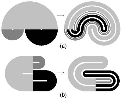
Figure 1: Illustration of action on a plane for the map suggested in the original paper of Plykin (a), and for the version of the map with the Plykin – Newhouse attractor (b). Each of them may be associated with a map defined on the sphere, say, by means of the stereographic projection

In the present article I show how the dynamics associated with attractor of Plykin type may be obtained in a system of coupled non-autonomous oscillators. As believed, it opens prospects for constructing physical and technical systems, e.g. electron devices with the structurally stable chaotic regimes.

In Section II a sequence of continuous transformations is defined on a two-dimensional sphere, and a system of two coupled oscillators is introduced, in which the state evolution corresponds in some sense to those transformations. The equations are written down for complex amplitudes of the oscillations. The points on the sphere represent the instantaneous states defined up to the overall phase factor. An explicit Poincaré map is derived that describes evolution of the state on one period of variation of coefficients in the non-autonomous differential equations. With exclusion of the overall phase, on which the evolution of other variables does not depend, the Poincaré map is reduced to a three-dimensional map, which possesses an attractor of Plykin type on an invariant sphere. In Section III results of computer verification of the so-called cone criterion are presented confirming the hyperbolic nature of the attractor of the three-dimensional map; it means also its structural stability. The topological type of the attractor corresponds to the construction of Plykin – Newhouse. In Section IV some results of numerical studies of the dynamics of the coupled oscillator system are discussed, including portraits of the attractor, Lyapunov exponents, power spectral density. In the set of equations for complex amplitudes, because of presence of a neutral direction in the state space, which is associated with the overall phase, the attractor has to be related formally to the class of partially hyperbolic ones 19 ; 6 .

II Representation of states on a sphere and equations describing dynamics of the model

Let us start with a system of two self-oscillators with compensation of losses from the common energy source. Let the equations for the slow amplitudes $a$ and $b$ read

$$\begin{array}[]{l}\dot{a}=\textstyle{1\over 2}\mu(1-|a|^{2}-|b|^{2})a,\\ \\ \dot{b}=\textstyle{1\over 2}\mu(1-|a|^{2}-|b|^{2})b,\\ \end{array}$$ (1)

where $\mu$ is a positive parameter. Let us set

$$\begin{array}[]{l}b=\sqrt{\rho}e^{i\varphi/2+i\psi}\sin(\theta/2),\\ \\ a=\sqrt{\rho}e^{-i\varphi/2+i\psi}\cos(\theta/2).\\ \end{array}$$ (2)

Clearly, in sustained regime of self-oscillations, the condition $\rho=|a|^{2}+|b|^{2}=1$ has to be valid. If we consider states satisfying $\rho=1$ and identify the states differing only in the overall phase, we can associate them with the points on a unit sphere (Fig. 2). Also, on the picture the Cartesian coordinates are shown:

$$\begin{array}[]{l}x=\rho\cos\varphi\sin\theta,\\ y=\rho\sin\varphi\sin\theta,\\ z=\rho\cos\theta.\\ \end{array}$$ (3)

Via the complex amplitudes they are expressed as

$$x+iy=2a^{\ast}b,\,\,\,z=|a|^{2}-|b|^{2}.$$ (4)

We intend to modify the model (1) in order to obtain a set of equations with coefficients periodically varying in time, in such way that in the stroboscopic description and in the representation on the unit sphere, the Plykin type attractor will occur.

As proved by Plykin, a uniformly hyperbolic attractor may exist on a sphere only in presence of at least four holes, the areas not visiting by trajectories belonging to the attractor. In our construction, the holes will correspond to neighborhoods of four points A, B, C, D, with coordinates $(x,y,z)=(\pm 1/\sqrt{2},\,\,0,\,\,\pm 1/\sqrt{2})$.

Let us consider a sequence of the following continuous transformations on the sphere:

• Flow down along circles of latitude, that is motion of the representative points on the sphere away from the meridians NABS and NDCS towards the meridians equally distant from the arcs AB and CD.

• Differential rotation around $z$-axis with angular velocity depending on z linearly, in such way that the points B and C do not move, while the points A and D exchange their location.

• Rotation of the sphere by $90^{\circ}$ around the $y$-axis.

• Flow down along circles of latitude, like at the first stage.

• Inverse differential rotation around $z$-axis.

• Inverse rotation by $90^{\circ}$ around the $y$-axis.

The procedure is symmetric in the sense that the operations for the stages (I) and (IV) are identical, while the stages (II) and (III) differ from (V) and (VI) only by directions of the rotations. Intuitively, it looks reasonable that this sequence of transformations will generate a flow on the sphere accompanying with formation of filaments of fine transversal structure, presence of which is a characteristic feature of the Plykin type attractors.

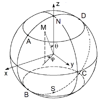
Figure 2: The unit sphere with marked points A, B, C, D, neighborhoods of which in the further construction will correspond to the holes not visiting by trajectories on the attractor. The north and south poles are indicated with N and S, respectively. The angular coordinates ($\theta$, $\varphi)$ are shown for some point M, and axes of the Cartesian coordinates $x$, $y$, $z$ are depicted

Let us construct equations for the complex amplitudes to reproduce dynamics on the above stages with corresponding motion of the points on the unit square representing the instantaneous states of the system. Duration of each of the six stages is accepted to be equal to a unit time interval.

On a stage of flow down along circles of latitude we require the angular velocity of motion on the sphere to be proportional to $\sin 2\varphi$. The simplest appropriate form of the differential equations is

$$\dot{a}=-i\varepsilon a\,\mbox{Im}({a^{*}}^{2}b^{2}),\,\,\,\dot{b}=i\varepsilon b\,\mbox{Im}({a^{*}}^{2}b^{2}).$$ (5)

Indeed, substituting $b=e^{i\varphi/2+i\psi}\sin(\theta/2)$ and $a=e^{-i\varphi/2+i\psi}\cos(\theta/2)$, after some simple transformations we get $\dot{\varphi}=\textstyle{1\over 2}\varepsilon\sin^{2}\theta\sin 2\varphi,\,\,\dot{\theta}=0$. Physically, the terms in the right-hand parts of (5) give rise to a frequency shift of opposite sign for two oscillators. Magnitude of the shift is proportional to the amplitude of a low-frequency signal generated by mixing of the second harmonic components from the oscillators on a quadrtatic nonlinear element.

On a stage of differential rotation, we set

$$\begin{array}[]{l}\dot{a}=\textstyle{1\over 4}i\sigma\pi(\sqrt{2}-1-2\sqrt{2}|a|^{2})a,\\ \\ \dot{b}=\textstyle{1\over 4}i\sigma\pi(\sqrt{2}+1-2\sqrt{2}|b|^{2})b,\end{array}$$ (6)

where $\sigma=\pm 1$. In angular variables $(\varphi,\,\,\theta)$, these equations reduce to $\dot{\varphi}=\textstyle{1\over 2}\sigma\pi(\sqrt{2}\cos\theta+1)$, $\,\dot{\theta}=0$. Note that the angular velocity $\dot{\varphi}$ depends linearly on $z=\cos\theta$ and vanishes at $z=-1/\sqrt{2}$. On this stage two subsystems must behave like uncoupled classic non-isochronous oscillators. At small amplitudes their frequencies in respect to the reference point are $\Delta\omega_{a,b}=\textstyle{1\over 4}i\sigma\pi(\sqrt{2}\mp 1)$. With growth of the amplitudes, the oscillation frequencies undergo a shift proportional to the squared amplitude for both subsystems.

Finally, on the stages of rotation an appropriate form of the equations is

$$\dot{a}=-\textstyle{1\over 4}\pi sb,\,\,\,\dot{b}=\textstyle{1\over 4}\pi sa,$$ (7)

where $s=\pm 1$. It corresponds to a conservative system of coupled oscillators with equal frequencies, with the coupling coefficient of such value that the energy exchange between the partial oscillators corresponds precisely to the duration of the stage.

Now, we can write down equations for the complex amplitudes embracing the complete time period $T=6$. For this, we compose the right-hand sides as combinations of terms (5), (6), (7), which are supposed to be switched in, or off, during the respective stages of the time evolution. As to the terms from the equations (1), we account them only on the stages of rotation. (Their exclusion for other stages is not so significant, but we do so, because it simplifies derivation of the Poincaré map in the explicit form.) Finally, we arrive at the equations

$$\begin{array}[]{c}\dot{a}=-i\varepsilon(1-\sigma^{2}-s^{2})\,\mbox{Im}(a^{2}b^{\ast 2})a-\textstyle{\pi\over 4}sb\\ +\textstyle{1\over 4}i\sigma\pi(\sqrt{2}-1-2\sqrt{2}|a|^{2})a\\ +\textstyle{1\over 2}s^{2}\mu(1-|a|^{2}-|b|^{2})a,\\ \\ \dot{b}=i\varepsilon(1-\sigma^{2}-s^{2})\,\mbox{Im}(a^{2}b^{\ast 2})b+\textstyle{\pi\over 4}sa\\ +\textstyle{1\over 4}i\sigma\pi(\sqrt{2}+1-2\sqrt{2}|b|^{2})b\\ +\textstyle{1\over 2}s^{2}\mu(1-|a|^{2}-|b|^{2})b.\\ \end{array}$$ (8)

Here the factors $\sigma$ and $s$ depend on time with period $T=6$, and on a single period they are defined by the relations

$$\sigma=\left\{{{\begin{array}[]{*{20}c}{-1,\,\,1\leq t<2\hfill}\\ {\,\,\,\,\,\,1,\,\,4\leq t<5,\hfill}\\ {\,\,\,\,\,\,0,\,\,{\rm otherwise,\hfill}}\\ \end{array}}}\right.\,\,\,s=\left\{{{\begin{array}[]{*{20}c}{-1,\,\,2\leq t<3\hfill}\\ {\,\,\,\,\,\,1,\,\,5\leq t<6,\hfill}\\ {\,\,\,\,\,\,0,\,\,{\rm otherwise.\hfill}}\\ \end{array}}}\right.$$ (9)

Let us derive the Poincaré map, which determines transformation of the state over one period $T=6$ and describes the time evolution stroboscopically.

Let the initial conditions for the equations (3) at $t_{n}=nT$ are defined as the state vector ${\rm{\bf X}}_{n}=(a_{n},b_{n})$, and the state after a half of period is ${\rm{\bf X}}_{n+1/2}={\rm{\bf F}}_{\sigma,s}({\rm{\bf X}}_{n})\quad=(a_{n+1/2},b_{n+1/2})$.

Solving equations (8) on each successive unit interval analytically, we can represent the map ${\rm{\bf F}}_{\sigma,s}$ explicitly:

$$\begin{array}[]{l}a_{n+1/2}=\frac{a_{n}De^{i\alpha+\mu/2}-sb_{n}D^{\ast}e^{i\beta+\mu/2}}{\sqrt{1+(|a_{n}|^{2}+|b_{n}|^{2})(e^{\mu}-1)}}\,\,,\\ \\ b_{n+1/2}=\frac{sa_{n}De^{i\alpha+\mu/2}+b_{n}D^{\ast}e^{i\beta+\mu/2}}{\sqrt{1+(|a_{n}|^{2}+|b_{n}|^{2})(e^{\mu}-1)}}\,\,,\\ \end{array}$$ (10)

where

$$\begin{array}[]{c}\alpha=\textstyle{1\over 4}\sigma\pi(\sqrt{2}-1-2\sqrt{2}|a_{n}|^{2}),\\ \\ \beta=\textstyle{1\over 4}\sigma\pi(\sqrt{2}+1-2\sqrt{2}|b_{n}|^{2}),\\ \\ D=\frac{1}{\sqrt{2}}\,\left({\frac{|a_{n}|^{2}|b_{n}|^{2}-(a_{n}^{*}b_{n})^{2}\tanh(2\varepsilon|a_{n}|^{2}|b_{n}|^{2})}{|a_{n}|^{2}|b_{n}|^{2}-(a_{n}b_{n}^{*})^{2}\tanh(2\varepsilon|a_{n}|^{2}|b_{n}|^{2})}}\right)^{1/4}.\\ \end{array}$$

The indices $\sigma$ and $s$ become equal $\pm 1$ alternately, so the mapping for the complete period is defined as follows:

$${\rm{\bf X}}_{n+1}={\rm{\bf F}}({\rm{\bf X}}_{n})={\rm{\bf F}}_{1,1}({\rm{\bf F}}_{-1,-1}({\rm{\bf X}}_{n})).$$ (11)

Dynamics governed by equations (8) or by iterations of the map (11) is invariant in respect to simultaneous constant phase shift for two oscillators, i.e. to the variable change $a\to ae^{i\psi},\,\,b\to be^{i\psi}$. Due to this, one can reduce the equations for two complex amplitudes to equations in three real variables.

Performing the variable change (4), we get a set of differential equations

$$\begin{array}[]{l}\begin{array}[]{r}\dot{x}=-\textstyle{1\over 2}\,\sigma\pi(z\sqrt{2}+1)y-\varepsilon(1-\sigma^{2}-s^{2})xy^{2}\\ +\textstyle{1\over 2}s\pi z+\mu s^{2}(1-\sqrt{x^{2}+y^{2}+z^{2}})x,\end{array}\\ \\ \begin{array}[]{r}\dot{y}=\textstyle{1\over 2}\sigma\pi(z\sqrt{2}+1)x/2+\varepsilon(1-\sigma^{2}-s^{2})yx^{2}\\ +\mu s^{2}(1-\sqrt{x^{2}+y^{2}+z^{2}})y,\end{array}\\ \\ \dot{z}=-\textstyle{1\over 2}s\pi x+\mu s^{2}(1-\sqrt{x^{2}+y^{2}+z^{2}})z,\\ \end{array}$$ (12)

where $\sigma$ and $s$ are time-dependent, as stated by formulas (9). Designating at $t_{n}=nT$ the state vector as ${\rm{\bf x}}_{n}=(x_{n},y_{n},z_{n})$, we can represent the three-dimensional Poincaré map as

$${\rm{\bf x}}_{n+1}={\rm{\bf f}}({\rm{\bf x}}_{n})={\rm{\bf f}}_{1,1}({\rm{\bf f}}_{-1,-1}({\rm{\bf x}}_{n})),$$ (13)

and the half-period map ${\rm{\bf x}}_{n+1/2}={\rm{\bf f}}_{\sigma,s}({\rm{\bf x}}_{n})$ is expressed as

$$\begin{array}[]{c}x_{n+1/2}=Psz_{n},\\ \\ y_{n+1/2}=PQ\left[{\sigma x_{n}e^{-\varepsilon(x_{n}^{2}+y_{n}^{2})/2}\sin\textstyle{\pi\over 2}(z_{n}\sqrt{2}+1)}\right.\\ \left.{+y_{n}e^{\varepsilon(x_{n}^{2}+y_{n}^{2})/2}\cos\textstyle{\pi\over 2}(z_{n}\sqrt{2}+1)}\right],\\ \\ \,z_{n+1/2}=PQ\left[{-sx_{n}e^{-\varepsilon(x_{n}^{2}+y_{n}^{2})/2}\cos\textstyle{\pi\over 2}(z_{n}\sqrt{2}+1)}\right.\\ \left.{+s\sigma y_{n}e^{\varepsilon(x_{n}^{2}+y_{n}^{2})/2}\sin\textstyle{\pi\over 2}(z_{n}\sqrt{2}+1)}\right],\\ \end{array}$$ (14)

where

$$\begin{array}[]{c}P=\left[{(1-e^{-\mu})\sqrt{x_{n}^{2}+y_{n}^{2}+z_{n}^{2}}+e^{-\mu}}\right]^{-1},\\ \\ Q=\frac{\sqrt{x_{n}^{2}+y_{n}^{2}}}{\sqrt{x_{n}^{2}e^{-\varepsilon(x_{n}^{2}+y_{n}^{2})}+y_{n}^{2}e^{\varepsilon(x_{n}^{2}+y_{n}^{2})}}}.\\ \end{array}$$

The maps (11) and (13) are reversible. The inverse maps are derived from solution of the equations (8) or (12) in the backward time; their analytic representations are omitted for brevity.

III Numerical results for the three-dimensional map and hyperbolic nature of the attractor

In Fig. 3 a-c portraits of the attractor are shown for the map ${\rm{\bf x}}_{n+1}={\rm{\bf f}}({\rm{\bf x}}_{n})$ at $\varepsilon=1$, $\mu=1$. They are obtained by computation of a sufficiently large number of iterations after excluding the initial transient part of the orbit. As seen from the diagram (a), in the space ($x$,$y$,$z$) the attractor is disposed on a unit sphere. In the diagram (b) it is represented in the angular coordinates $(\varphi,\,\,\theta)$, and in the diagram (c) as an object on the plane of the complex variable

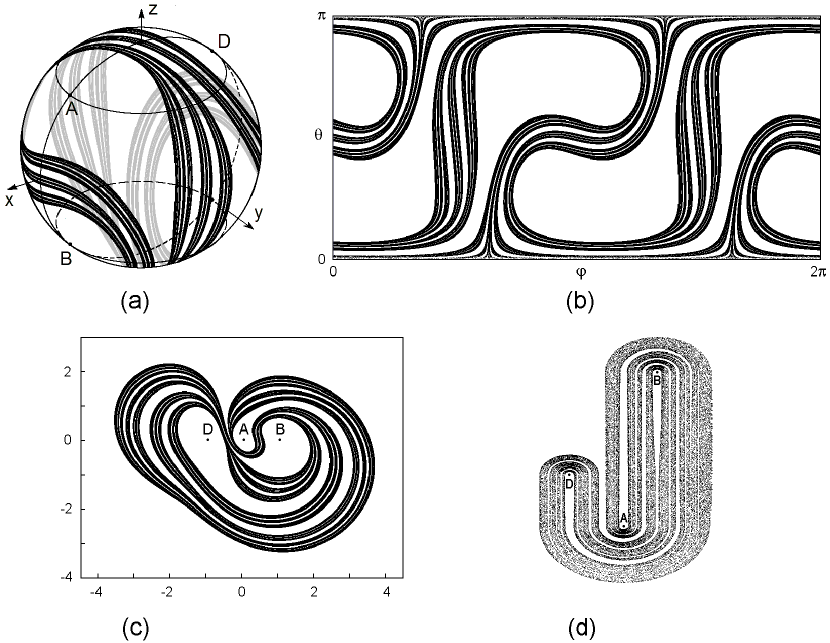
Figure 3: Attractor of the map (13) at $\varepsilon=1$ and $\mu=1$ in three-dimensional space on the unit square (a), its representation in the angular coordinates $(\varphi,\,\,\theta)$ (b), and a portrait on the plane in stereographic projection (c). Panel (d) shows for comparison the portrait of the Plykin – Newhouse attractor reproduced from Ref. 20 for the Hunt model 18 . The orientation is selected specially to see better the correspondence of the structure of the filaments with that in the diagram (c)

$$W=\frac{x-z+iy\sqrt{2}}{x+z+\sqrt{2}}.$$ (15)

The last corresponds to stereographic projection from the sphere to the plane with a use of the point $C$ as a center. This point together with a neighborhood does not belong to the attractor of the map; so, its image occupies a bounded part of the plane $W$.

Note specific fractal-like transverse structure of the attractor. Few initial levels of this structure are easily distinguishable: the object looks like composed of strips, each of which contains narrower strips of the next level etc. As follows from the computations discussed below, it is a uniformly hyperbolic strange attractor. Its topological type corresponds to the Plykin – Newhouse attractor. The last follows from visual comparison of mutual location of filaments in the diagram (c) and in the Plykin – Newhouse attractor shown in diagram (d). (The last picture is taken from the paper 20 , which reproduces analysis of the Hunt model 18 , definitely possessing the attractor of Plykin – Newhouse.)

To compute all Lyapunov exponents for the three-dimensional map, joint iterations of (13) together with a collection of three equations in variations for perturbation vectors are produced. At each step, Gram–Schmidt process is applied to obtain an orthogonal set of vectors, and normalization of the vectors to a fixed constant is performed. Lyapunov exponents are obtained as slopes of the straight lines approximating the accumulating sums of logarithms of the norm ratios for the vectors in dependence of the number of iterations 21 . In particular, at $\varepsilon=1$ and $\mu=1$ the Lyapunov exponents are, $\Lambda_{1}=0.9575$, $\Lambda_{2}=-1.2520$, $\Lambda_{3}=-2$, and estimate of the attractor dimension with the Kaplan – Yorke formula yields $D_{L}=1+\Lambda_{1}/|\Lambda_{2}|\approx 1.765$.

To substantiate the hyperbolic nature of the attractor, let us turn to computational verification of the cone criterion known from the mathematical literature 6 ; 7 ; 8 ; 22 ; 18 ; 14 .

Let us have a smooth map ${\rm{\bf\bar{x}}}={\rm{\bf g}}({\rm{\bf x}})$ that determines discrete-time dynamics on an attractor $A$.

The criterion requires that with appropriate selection of a constant $\gamma>1$, for any point ${\rm{\bf x}}\in A$, in the space of vectors of infinitesimal perturbations one can define the expanding and contracting cones $S_{\rm{\bf x}}$ and $C_{\rm{\bf x}}$. Here $S_{\rm{\bf x}}$ is a set of vectors satisfying the condition that their norms increase by factor $\gamma$ or more under the action of the map. $C_{\rm{\bf x}}$ is a set of vectors, for which the norms increase by factor $\gamma$ or more under the action of the inverse map ${\rm{\bf\tilde{x}}}={\rm{\bf g}}^{-1}({\rm{\bf x}})$. The cones $S_{\rm{\bf x}}$ and $C_{\rm{\bf x}}$ must be invariant in the following sense. (i) For any ${\rm{\bf x}}\in A$ the image of the expanding cone from the pre-image point ${\rm{\bf\tilde{x}}}$ must be a subset of the expanding cone at x. (ii) For any ${\rm{\bf x}}\in A$ the pre-image of the contracting cone from the image point ${\rm{\bf\bar{x}}}$ must be a subset of the contracting cone at x.

Let ${\rm{\bf g}}({\rm{\bf x}})$ be a map corresponding to the $k$-fold iteration of the Poincaré map ${\rm{\bf f}}^{k}({\rm{\bf x}})$, where $k$ is an integer selected in the course of the computations. The needed Jacobian matrices can be found in our case analytically, by differentiating of (13) with application of the chain rule for the derivatives of the functional compositions. Some details of the computational procedure, which takes into account disposition of the attractor on the invariant sphere, are given in Appendix.

The calculations are organized as verification of the required conditions for a set of point on the attractor obtained from multiple iterations of the map ${\rm{\bf g}}({\rm{\bf x}})$. We check, first, the existence of nonempty expanding and contracting cones, and secondly, the validity of inequalities corresponding to proper inclusions of these cones. If these conditions are met with $\gamma=1$, the interval, is determined $\gamma_{\min}({\rm{\bf x}})\leq\gamma\leq\gamma_{\max}({\rm{\bf x}})$, in which they are true.

Figure 4 shows a diagram resuming graphically results of verification of the cone criterion for the attractor of the map (13) at $\varepsilon=1$ and $\mu=1$. The computations have been performed for the map ${\rm{\bf f}}^{3}({\rm{\bf x}})$. The diagram represents in logarithmic scale the values $\gamma_{\min}({\rm{\bf x}})$ in gray and $\gamma_{\max}({\rm{\bf x}})$ in black versus $y$ coordinate of the analyzed points on the attractor. Observe a gray set and a black set, one disposed strongly above, and another strongly below the horizontal line $\gamma=1$. Presence of a gap separating these sets from the line $\gamma=1$ implies the positive result of the test. To express the result quantitatively, one can determine the maximum of $\gamma_{\min}({\rm{\bf x}})$ and minimum of $\gamma_{\max}({\rm{\bf x}})$ over the set of all processed points. As found, selection of the constant satisfying $0.44<\gamma^{2}<2.3$ ensures the required invariance of the cones.

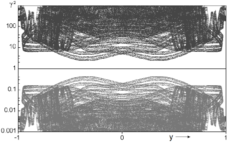
Figure 4: A graphical illustration for verification of the hyperbolic nature of the attractor for the map (13), with $\varepsilon$=1 and $\mu$=1. A positive result of the test follows from existence of the gap between the line $\gamma=1$ and the black and gray sets of points, which represent, respectively, the upper and lower edges of the intervals of $\gamma$, which met the verified conditions

IV Numerical results for the coupled oscillators

In accordance with the previous section, there is a correspondence between dynamics of complex amplitudes in the coupled oscillators (8) and dynamics of the three-dimensional mapping (13) possessing the hyperbolic attractor of Plykin – Newhouse. Let us illustrate with numerical results the dynamics of the coupled oscillators concentrating on features linked with the flow nature of the system, i.e. with the continuous time evolution.

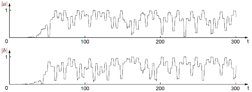
Figure 5: Plots of the real amplitudes $|a|$ and $|b|$ versus time in the transient process obtained from numerical solution of the differential equations (8) at $\varepsilon$=1 and $\mu$=1

Figure 5 shows plots for the amplitudes of the coupled oscillators $|a|$ and $|b|$ versus time obtained from numerical solution of the differential equations (8) with the Runge – Kutta method at $\varepsilon=1$ and $\mu=1$. Some small in absolute value and random in phase complex amplitudes $a$ and $b$ are taken as initial conditions, so the plot depicts the transient process prior to the regime of chaotic self-oscillations. In the right-hand part of the diagram the dependences look like samples of a random process; that associates with motion on the chaotic attractor. Locally, some peculiarities can be seen because of the piecewise continuous nature of the process composed of successive stages. In particular, the horizontal plateaus relate to the stages of evolution, on which the amplitudes $|a|$ and $|b|$ remain constant according to equations (6). Note that the realizations for $|a|$ and $|b|$ are interconnected: in the sustained regime they obey the relation $|a|^{2}+|b|^{2}=1$.

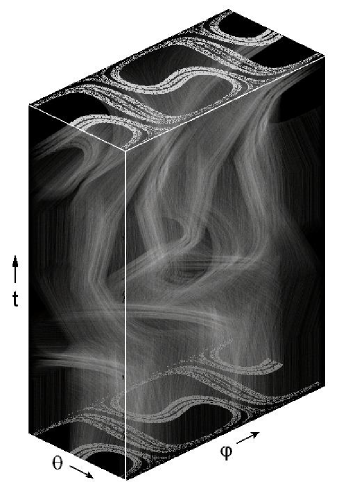
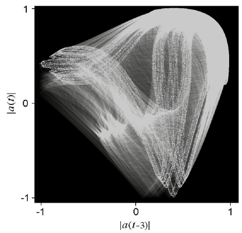
Figure 6: (a) Portrait of attractor for the system (8) in three-dimensional space $(\varphi,\theta,\,\,t)$. In the cross-section with the horizontal plane $t=0\,\,(\bmod 6)$ observe the object identical to that shown in Fig. 3 b. (b) Portrait of the attractor in the plane of real amplitudes relating to one of the oscillators and separated by time interval $T$/2=3. Technique of representation in gray scales is used: brighter tones correspond to higher probability of visiting the pixels by the representative points. The parameter values are $\varepsilon$=1, $\mu$=1

Figure 6 presents two versions of portraits of the attractor for the system (8) at $\varepsilon=1$ and $\mu=1$. As the dimension of the state space is sufficiently high (vector ${\rm{\bf X}}=(a,b)$ is four-dimensional, and the extended state space of the non-autonomous system is five-dimensional), depicting the image to resolve subtle fractal transverse structure intrinsic to the attractor is not a trivial task. For this, we apply presentation of the object in gray scales. Brighter tones correspond to pixels visiting by the representative point with higher probability 23 . In panel (a) this technique is used to draw the three-dimensional portrait. Angular coordinates $(\varphi,\theta)$ are plotted in a horizontal plane. The third variable plotted along the vertical axis is time, within one full period of variation of coefficients in the equations (8). The picture reminds rising and swirling smoke. In the cross-section with a horizontal plane $t=0\,\,(\bmod 6)$ observe a fractal-like formation identical to the attractor of the three-dimensional map depicted in angular coordinates in Fig. 3 b. One more portrait is shown in the panel (b) on the plane of two values of real amplitude $|a(t)|$ and $|a(t-3)|$, which relate to instants separated by a half of time period of variation of the coefficients in the equations (8). Here, again one can distinguish the fractal-like transverse structure linked with the dynamics of the Plykin type. This method of visualization may be appropriate in experiments with systems of the class under consideration.

The Lyapunov exponents $\lambda_{i}$ of equations (8) are linked with the exponents for the Poincaré map (see (10), (11)) by an evident relation $\lambda_{i}=\Lambda_{i}/T$, where $T=6$ is the period of variation of the coefficients in the equations. The procedure of computation of the Lyapunov exponents $\Lambda_{i}$ is analogous to that used for the three-dimensional map. Joint iterations of the map (11) together with a collection of four equations in variations are produced. At each step, Gram–Schmidt process is applied to the set of vectors, and normalization of them to a fixed constant is performed. Figure 7 present the results graphically. The first plot (a) shows four Lyapunov exponents $\Lambda_{i}$ in dependence on parameter $\varepsilon$ at fixed $\mu=1$. In the range $\varepsilon<\varepsilon_{c}\approx 2.03$ one of the exponents is positive that means chaos. Among other exponents one is zero (up to numerical errors), and two are negative. Note a smooth dependence of the largest exponent on the parameter. For larger $\varepsilon$ (strong dissipation bringing in during the flow down stages) chaos disappears. The second plot (b) shows the Lyapunov exponents versus $\mu$ at fixed $\varepsilon=1$. Observe that variation of $\mu$ notably effects only one exponent, which corresponds, obviously, to approach of orbits to the invariant sphere. Presence of a zero exponent reflects invariance of the equations in respect to the overall phase shift. Of course, results of computations agree with the data from the previous section: at identical $\varepsilon$ and $\mu$ three nonzero exponent are equal, up to numerical errors, to those obtained for the three-dimensional map.

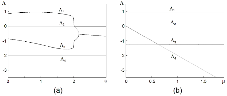
Figure 7: Four Lyapunov exponents versus parameter $\varepsilon$ at $\mu=1$ (a) and versus parameter $\mu$ at $\varepsilon=1$ (b) for the Poincaré map represented in terms of complex amplitudes. A zero exponent occurs due to invariance of the equations in respect to the overall phase shift

Figure 8 shows a plot of spectral density in logarithmic scale versus a frequency for a signal generated by one of the oscillators. It relates to regime of dynamics on the Plykin – Newhouse attractor interpreted in terms of the three-dimensional map. This spectrum is one more characteristic interesting in the context of possible experiments.

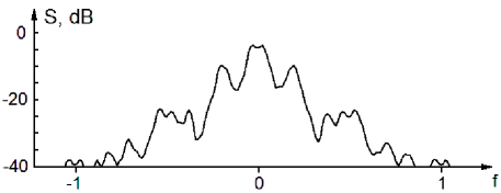
Figure 8: The power spectral density for one of the coupled oscillators versus the frequency computed by processing a realization obtained from numerical integration of the equations (8) at $\varepsilon=1$ and $\mu=1$

In computations the standard methodic was used recommended for non-parametric statistical estimates of the power spectral density. It is based on subdividing the whole realization on a number of parts of equal duration. For each part, the signal is multiplied by a smooth function vanishing at the ends of the interval (‘window’), then Fourier transform is applied, and finally, the squared amplitudes of the frequency components are averaged over all the parts. A sample of the time series for the complex variable $a(t)$ was obtained from numerical solution of equations (8) by the finite-difference method. It corresponds to motion on the attractor and contains $6\cdot 10^{5}$ data points with time step $\Delta t=0.01$. As seen from the picture, the spectrum looks continuous that corresponds to chaotic nature of the generated signal. The spectrum is almost perfectly symmetric about the reference frequency, where the spectral density is maximal. The two main side maximums have a level below the central one by about 7 dB, and their frequencies approximately correspond to the inverse value of the period of variation of the coefficients in equations (8): $f\approx\pm 1/6$. Apparently, this periodicity is a reason for the rugged form of the spectrum. A plot for the power spectral density for the second oscillator looks exactly the same because of the symmetry of the system.

V Conclusion and discussion

In the present article a system of two coupled non-autonomous nonlinear oscillator is introduced manifesting chaotic dynamics, which is in a direct relation with the concepts of the hyperbolic theory. With exclusion of the overall phase the Poincaré map reduces to a three-dimensional map possessing attractor of Plykin type disposed on an invariant sphere.

As the systems of coupled oscillators occur in many fields in physics and technology, it is natural to expect that the suggested model may be realizable. Particularly, it may relate to electronic devices, mechanical systems, objects of laser physics and nonlinear optics. The systems with hyperbolic chaos may be of special interest for applications due to their robustness, or structural stability, that means insensitivity of the devices to variations of parameters, characteristics of elements, technical fluctuations, noise etc.

Appearance of concrete examples of systems with hyperbolic strange attractors makes it reasonable to apply for them the whole arsenal of computational methods accumulated in nonlinear dynamics and its applications. This is of evident interest both from the point of view of complementation of the mathematical concepts with concrete and visible context (see e.g. a paper 25 ), and for exploiting these concepts in applications. In the present work such results of computer studies are presented as realizations, attractor portraits, Lyapunov exponents, estimate of dimension, power spectral density.

It is worth mentioning some possible modifications of the model.

• It is easy to suggest a version of the equations, in which the temporal dependence of the coefficients will be piecewise smooth. For this, one can introduce in the equations ${\rm{\bf\dot{x}}}={\rm{\bf f}}({\rm{\bf x}},t)$ a smooth common time-dependent factor vanishing at the junctions of the stages, integral of which over a stage duration equals 1. An appropriate variant is ${\rm{\bf\dot{x}}}=(2\sin^{2}\pi t){\rm{\bf f}}({\rm{\bf x}},t)$. The Poincaré map remains the same, and the nature of the attractor is not changed too. (Hunt used a similar trick in his thesis 18 .)

• As mentioned, the “self-oscillatory” term in the equations proportional to $\mu$ may be retained on all stages of the dynamics.

• Working with a version of the model describing by the three-dimensional set of equations, it is possible to simplify the form of the nonlinearity excluding the operation of extracting the square root, and setting the respective term to be $\mu(1-x^{2}-y^{2}-z^{2})$. This modification does not influence dynamics on the attractor belonging to the invariant set $x^{2}+y^{2}+z^{2}=1$. (In amplitude equations for $a$ and $b$ such modification leads rather to complication because of increase of degree of the nonlinear terms.)

• Taking into account structural stability of the hyperbolic attractor, many other modifications can be done, which do not change the nature of the attractor, while the variations are not too large. In particular, it is possible to introduce a model with smooth analytical variation of the coefficients in time in the non-autonomous equations 24 .

Formally, in our complex amplitude equations the attractor should not be interpreted as uniformly hyperbolic, because of presence of a neutral direction in the state space associated with the overall phase. Instead, it has to be related to the class of partially hyperbolic attractors 19 ; 6 . Nevertheless, in the form used here invariance of the equations in respect to the overall phase is exact; it means that one can accept a rightful agreement not to distinguish states distinct only in the phase, and, in this sense, treat the dynamics as true hyperbolic.

However, in systems, for which description in terms of slow complex amplitudes will be an approximation, one can expect appearance of peculiarities associated with features of the partially hyperbolic attractor. If the deflections from the slow-amplitude approximation are small, the overall phase will manifest slow random walk, while the dynamics of the rest variables will retain its character because of intrinsic robustness.

In dependence on parameters, the suggested model can manifest chaos and regular (periodic) dynamics. So, it may serve as an object for principal and interesting studies of scenarios of the onset of hyperbolic strange attractors in the course of parameter variations (see e.g. 26 ; 27 ). Insufficient progress in this research direction may be explained particularly by the fact that no realistic examples of concrete systems undergoing such transitions were known.

The work was performed under support of RFBR – DFG grant No 08-02-91963.

Appendix

For a three-dimensional dissipative map ${\rm{\bf\bar{x}}}={\rm{\bf g}}({\rm{\bf x}})$, ${\rm{\bf x}},\,{\rm{\bf\bar{x}}}\in R^{3}$ let us consider the procedure for verification of the cone criterion, bearing in mind the situation that one expanding and two contracting directions present in the state space, and the attractor is located on the invariant sphere. The map is supposed to be reversible: any state vector x has a unique image ${\rm{\bf\bar{x}}}={\rm{\bf g}}({\rm{\bf x}})$ and a unique pre-image ${\rm{\bf\tilde{x}}}={\rm{\bf g}^{-1}}({\rm{\bf x}})$.

Let the derivative matrix of the map g at x be ${\rm{\bf v}}={\rm{\bf d}}_{\rm{\bf x}}({\rm{\bf g}})$, which acts in the tangent space of vectors ${\rm{\bf u}}=\left\{{u_{1},u_{2},u_{3}}\right\}$. Via the auxiliary symmetric matrix ${\rm{\bf\hat{b}}}={\rm{\bf v}}^{\rm{\bf T}}{\rm{\bf v}}$, where the superscript T means the transpose, the norm of the vector ${\rm{\bf\bar{u}}}={\rm{\bf vu}}$ is expressed as

$$\left\|{\rm{\bf\bar{u}}}\right\|^{2}={\rm{\bf u}}^{\rm{\bf T}}{\rm{\bf\hat{b}u}}.$$ (16)

The expanding cone at the point x is a set of vectors

$$S_{\rm{\bf x}}=\left\{{{\rm{\bf u}}\,\left|{\,{\rm{\bf u}}^{\rm{\bf T}}{\rm{\bf\hat{b}u}}\geq\gamma^{2}{\rm{\bf u}}^{\rm{\bf T}}{\rm{\bf u}}}\right.}\right\}.$$ (17)

With the same matrix ${\rm{\bf\hat{b}}}$ one can define a pre-image of the contracting cone relating to the point ${\rm{\bf\bar{x}}}={\rm{\bf g}}({\rm{\bf x}})$, namely,

$${C}^{\prime}_{\rm{\bf x}}=\left\{{{\rm{\bf u}}\,\left|{\,\gamma^{2}{\rm{\bf u}}^{\rm{\bf T}}{\rm{\bf\hat{b}u}}\leq{\rm{\bf u}}^{\rm{\bf T}}{\rm{\bf u}}}\right.}\right\}.$$ (18)

Now, let us consider an inverse map ${\rm{\bf\tilde{x}}}={\rm{\bf g}}^{-1}({\rm{\bf x}})$ and its matrix derivative ${\rm{\bf w}}={\rm{\bf d}}_{\rm{\bf x}}({\rm{\bf g}}^{-1})$. Via the auxiliary symmetric matrix ${\rm{\bf\hat{a}}}={\rm{\bf w}}^{\rm{\bf T}}{\rm{\bf w}}$ we represent the norm of the vector ${\rm{\bf\tilde{u}}}={\rm{\bf wu}}$ as

$$\left\|{\rm{\bf\tilde{u}}}\right\|^{2}={\rm{\bf u}}^{\rm{\bf T}}{\rm{\bf\hat{a}u}}.$$ (19)

With the matrix ${\rm{\bf\hat{a}}}$ we define the contracting cone at x as a set

$$C_{\rm{\bf x}}=\left\{{{\rm{\bf u}}\,\left|{\,{\rm{\bf u}}^{\rm{\bf T}}{\rm{\bf\hat{a}u}}\geq\gamma^{2}{\rm{\bf u}}^{\rm{\bf T}}{\rm{\bf u}}}\right.}\right\},$$ (20)

and a cone that is an image of the expanding cone relating to the point ${\rm{\bf\tilde{x}}}={\rm{\bf g}}^{-1}({\rm{\bf x}})$, namely,

$${S}^{\prime}_{\rm{\bf\tilde{x}}}=\left\{{{\rm{\bf u}}\,\left|{\,\gamma^{2}{\rm{\bf u}}^{\rm{\bf T}}{\rm{\bf\hat{a}u}}\leq{\rm{\bf u}}^{\rm{\bf T}}{\rm{\bf u}}}\right.}\right\}.$$ (21)

In computations it is necessary to check, first, existence of nonempty cones satisfying the definitions, and, second, validity of the inclusions ${S}^{\prime}_{\rm{\bf\tilde{x}}}\subset S_{\rm{\bf x}}$ and ${C}^{\prime}_{\rm{\bf\bar{x}}}\subset C_{\rm{\bf x}}$.

As the attractor is placed on an invariant sphere $S^{2}$, let us assume that ${\rm{\bf x}}\in S^{2}$. To define a convenient orthogonal basis $\left\{{{\rm{\bf i}}_{1},{\rm{\bf i}}_{2},{\rm{\bf i}}_{3}}\right\}$ we take as ${\rm{\bf i}}_{3}$ a unit vector directed along the radius at x, and the unit vectors ${\rm{\bf i}}_{1},\,\,{\rm{\bf i}}_{2}$ are taken in the tangent plane. To be concrete, we require the matrix element $\hat{b}_{12}$ to vanish, and the inequality $\hat{b}_{11}>\hat{b}_{22}$ to hold.

The conditions of required inclusion of the cones are formulated in terms of quadratic forms associated with the matrices ${\rm{\bf b}}={\rm{\bf\hat{b}}}-\Gamma^{2}{\rm{\bf\hat{e}}}$ and ${\rm{\bf a}}={\rm{\bf\hat{a}}}-\Gamma^{2}{\rm{\bf\hat{e}}}$, where ${\rm{\bf\hat{e}}}$ is the unite matrix. A constant factor $\Gamma$ is assumed to be equal $\gamma$, or 1/$\gamma$, considering the expanding, or contracting cones, respectively. Note that the matrices a and b are symmetric: $b_{ij}=b_{ji},\,\,a_{ij}=a_{ji}$.

Equations

$$b_{11}u_{1}^{2}+b_{22}u_{2}^{2}+b_{33}u_{3}^{2}+2b_{13}u_{1}u_{3}+2b_{23}u_{2}u_{3}=0$$ (22)

and

$$a_{11}u_{1}^{2}+a_{22}u_{2}^{2}+a_{33}u_{3}^{2}+2a_{12}u_{1}u_{2}+2a_{13}u_{1}u_{3}+2a_{23}u_{2}u_{3}=0$$ (23)

determine the borders of the cones. By variable change

$${u}^{\prime}_{1}=u_{1}+b_{11}^{-1}b_{13}u_{3},\,\,\,{u}^{\prime}_{2}=u_{2}+b_{22}^{-1}b_{23}u_{3},\,\,\,{u}^{\prime}_{3}=u_{3}$$ (24)

the quadratic form in (22) is reduced to a standard form:

$$b_{11}{u^{\prime}}_{1}^{2}+b_{22}{u^{\prime}}_{2}^{2}+{b}^{\prime}_{33}{u^{\prime}}_{3}^{2}=0,$$ (25)

while the equation (23) becomes

$$\begin{array}[]{c}a_{11}{u^{\prime}}_{1}^{2}+a_{22}{u^{\prime}}_{2}^{2}+{a}^{\prime}_{33}{u^{\prime}}_{3}^{2}+\\ +2a_{12}{u^{\prime}}_{1}{u^{\prime}}_{2}+2{a}^{\prime}_{13}{u^{\prime}}_{1}{u^{\prime}}_{3}+2{a}^{\prime}_{23}{u^{\prime}}_{2}{u^{\prime}}_{3}=0.\end{array}$$ (26)

Here

$$\,\,{b}^{\prime}_{33}=b_{33}-b_{11}^{-1}b_{13}^{2}-b_{22}^{-1}b_{23}^{2}$$ (27)

and

$$\begin{array}[]{c}{a}^{\prime}_{13}=a_{13}-a_{11}b_{11}^{-1}b_{13}-a_{12}b_{22}^{-1}b_{23},\\ \\ {a}^{\prime}_{23}=a_{23}-a_{12}b_{11}^{-1}b_{13}-a_{22}b_{22}^{-1}b_{23},\\ \\ {a}^{\prime}_{33}=a_{33}+a_{11}b_{11}^{-2}b_{13}^{2}+a_{22}b_{22}^{-2}b_{23}^{2}-2a_{13}b_{11}^{-1}b_{13}\\ -2a_{23}b_{22}^{-1}b_{23}+2a_{12}b_{11}^{-1}b_{13}b_{22}^{-1}b_{23}.\\ \end{array}$$ (28)

In the cross-section by a plane $u^{\prime}_{1}={\rm const}$ the equations (25) and (26) determine some curves of the second order; their types and mutual location have to be revealed in the course of computations. To have situation of inclusion required by the criterion, these curves must be ellipses.

First, in computations we check the inequalities $b_{11}>0,\,\,\,b_{22}<0,\,\,\,{b}^{\prime}_{33}<0$. If they are true, the equation (25) defines an ellipse.

To determine the type of the curve given by (26), we compute the invariants

$$I=a_{22}+{a}^{\prime}_{33},\,D=\left|{{\begin{array}[]{*{20}c}{a_{22}\hfill}&{{a}^{\prime}_{23}\hfill}\\ {{a}^{\prime}_{23}\hfill}&{{a}^{\prime}_{33}\hfill}\\ \end{array}}}\right|,\,\,A=\left|{{\begin{array}[]{*{20}c}{a_{11}\hfill}&{a_{12}\hfill}&{{a}^{\prime}_{13}\hfill}\\ {a_{12}\hfill}&{a_{22}\hfill}&{{a}^{\prime}_{23}\hfill}\\ {{a}^{\prime}_{13}\hfill}&{{a}^{\prime}_{23}\hfill}&{{a}^{\prime}_{33}\hfill}\\ \end{array}}}\right|$$ (29)

and check that $D>0$, and $A/I>0$. Then, in accordance with the theory of conic sections, the equation (26) also defines an ellipse.

Let us formulate a convenient and simple sufficient condition of location of the second ellipse inside the first one. Renormalizing variables

$$\xi=\sqrt{b_{11}}u^{\prime}_{1},\,\,\,\eta=\sqrt{-b_{22}}u^{\prime}_{2},\,\,\,\zeta=\sqrt{-b_{33}}u^{\prime}_{3}$$ (30)

and setting $u^{\prime}_{1}=1/\sqrt{b_{11}}$, transforms the first ellipse to a unit circle

$$\eta^{2}+\zeta^{2}=1.$$ (31)

Then, the equation for the second ellipse is

$$\begin{array}[]{c}-\frac{a_{22}}{b_{22}}\eta^{2}+\frac{2{a}^{\prime}_{23}}{\sqrt{b_{22}{b}^{\prime}_{33}}}\eta\zeta-\frac{{a}^{\prime}_{33}}{{b}^{\prime}_{33}}\zeta^{2}+\frac{2a_{12}}{\sqrt{-b_{11}b_{22}}}\eta\\ +\frac{2{a}^{\prime}_{13}}{\sqrt{-b_{11}{b}^{\prime}_{33}}}\zeta+\frac{a_{11}}{b_{11}}=0,\end{array}$$ (32)

and its center is located at

$$\begin{array}[]{l}\eta_{0}=\,\frac{a_{12}{a}^{\prime}_{33}+{a}^{\prime}_{13}{a}^{\prime}_{23}}{a_{22}{a}^{\prime}_{33}-{{a}^{\prime}_{23}}^{2}}\sqrt{-\frac{b_{22}}{b_{11}}},\\ \\ \zeta_{0}=\,\frac{{a}^{\prime}_{13}a_{22}+a_{12}{a}^{\prime}_{23}}{a_{22}{a}^{\prime}_{33}-{{a}^{\prime}_{23}}^{2}}\sqrt{-\frac{{b}^{\prime}_{33}}{b_{11}}}.\end{array}$$ (33)

In variables $\tilde{\eta}=\eta-\eta_{0},\,\,\tilde{\zeta}=\zeta-\zeta_{0}$ the equation becomes

$$-\frac{a_{22}}{b_{22}}\tilde{\eta}^{2}+\frac{2{a}^{\prime}_{23}}{\sqrt{b_{22}{b}^{\prime}_{33}}}\tilde{\eta}\tilde{\zeta}-\frac{{a}^{\prime}_{33}}{{b}^{\prime}_{33}}\tilde{\zeta}^{2}=R^{2},$$ (34)

where

$$\begin{array}[]{c}R^{2}=-\frac{a_{11}}{b_{11}}+\frac{a_{22}}{b_{22}}\eta_{0}^{2}-\frac{2{a}^{\prime}_{23}}{\sqrt{b_{22}{b}^{\prime}_{33}}}\eta_{0}\zeta_{0}+\frac{{a}^{\prime}_{33}}{{b}^{\prime}_{33}}\zeta_{0}^{2}\\ \\ -\frac{2a_{12}}{\sqrt{-b_{11}b_{22}}}\eta_{0}-\frac{2{a}^{\prime}_{13}}{\sqrt{-b_{11}{b}^{\prime}_{33}}}\zeta_{0}.\end{array}$$ (35)

Computing the lesser root of the square equation

$$l^{2}+(a_{22}/b_{22}+{a}^{\prime}_{33}/{b}^{\prime}_{33})l+(a_{22}{a}^{\prime}_{33}-4{{a}^{\prime}_{23}}^{2})/(b_{22}{b}^{\prime}_{33})=0,$$ (36)

one finds out the semi-major axis $R/\sqrt{l_{\min}}$. A sufficient condition for the ellipse to be located inside the unit disc is inequality

$$\sqrt{\eta_{0}^{2}+\zeta_{0}^{2}}\,+R/\sqrt{l_{\min}}<1.$$ (37)

If all the named conditions are true at $\Gamma=\gamma$ and at $\Gamma=1/\gamma$, one can deduce about the correct inclusion for the expanding and contracting cones at the analyzed point x.

Indeed, in variables $\eta$, $\zeta$ the cross-section of the expanding cone $S_{\rm{\bf x}}$ is the closed unit disc, and cross-section of the cone ${S}^{\prime}_{\rm{\bf\tilde{x}}}$ is represented by the closure of interior of the small ellipse obtained at $\Gamma=\gamma$, so, the required inclusion ${S}^{\prime}_{\rm{\bf\tilde{x}}}\subset S_{\rm{\bf x}}$ is valid (Fig. 9 a). On the other hand, cross-section of the contracting cone $C_{\rm{\bf x}}$ is a closure of exterior of the small ellipse obtained at $\Gamma=1/\gamma$. Cross-section of the cone ${C}^{\prime}_{\rm{\bf\bar{x}}}$ corresponds to a closure of exterior of the unit circle. Hence, the inclusion ${C}^{\prime}_{\rm{\bf\bar{x}}}\subset C_{\rm{\bf x}}$ is valid (Fig. 9 b).

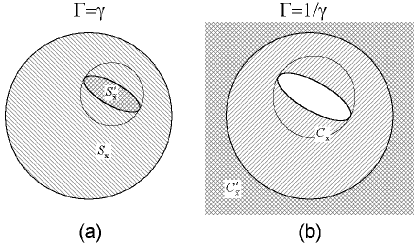
Figure 9: Cross-sections of the cones for the case of three-dimensional map with one expanding and two contracting directions. A picture of proper inclusion is shown (a) for expanding cones ${S}^{\prime}_{\rm{\bf\tilde{x}}}\subset S_{\rm{\bf x}}$ and (b) for contracting cones ${C}^{\prime}_{\rm{\bf\bar{x}}}\subset C_{\rm{\bf x}}$ A circle circumscribed around the ellipse is located inside the unit disc if the condition (19) is valid

Computations in the present work were organized as verification of the cone criterion for a set of points on the attractor obtained from multiple iterations of the map ${\rm{\bf g}}({\rm{\bf x}})$. The inclusions were checked with a help of the inequality (37).

Because of smoothness of the map under study, the objects considered in the context of the cone criterion (matrices, quadratic forms and their invariants) depend on the state variables in smooth manner, as they are determined by dynamics on finite time intervals. As follows, validity of the conditions at some point x with distant from 1 constant $\gamma$ implies that the cone criterion holds as well in a neighborhood of x (as wider, as larger the value $|\gamma-1|$ is). A positive result of the test for a representative set of points implies validity of the cone criterion on the whole attractor, if it is completely covered by the union of the mentioned neighborhoods. Practically, such situation is achieved by increase of the number of iterations and, respectively, a number of tested points on the attractor.

It is convenient not to fix in advance the constant $\gamma$, but to arrange the computations as follows. First, at each point x we compute the matrices ${\rm{\bf\hat{a}}}$ and ${\rm{\bf\hat{b}}}$ and check all the formulated conditions for $\gamma=1$. If they hold, the program determines an allowable interval of $\gamma$. For this, the program simply enumerates the $\gamma$ values with a small step in a sufficiently wide range. Attractor is recognized as hyperbolic if a gap of a finite width separates the obtained sets of top and bottom edges of the intervals from the axis $\gamma=1$ on the plot of $\gamma$ versus some dynamical variable characterizing location of the analyzed point x.

References

- (1) J.-P. Eckmann and D. Ruelle, Rev. Mod. Phys. 57, 617 (1985).
- (2) R.L. Devaney, An Introduction to Chaotic Dynamical Systems (Addison-Wesley, New York, 1989).
- (3) L. Shilnikov, International Journal of Bifurcation and Chaos. 7, 1353 (1997).
- (4) J. Guckenheimer and P. Holmes, Nonlinear Oscillations, Dynamical Systems, and Bifurcations of Vector Fields (Springer, 2002).
- (5) L.P. Shilnikov, A.L. Shilnikov, D.V. Turaev, L.O. Chua, Methods of Qualitative Theory in Nonlinear Dynamics (World Scientific Publ., Singapore, 1998).
- (6) A. Katok and B. Hasselblatt, Introduction to the Modern Theory of Dynamical Systems (Cambridge University Press, 1995).
- (7) V. Afraimovich. and S.-B. Hsu, Lectures on chaotic dynamical systems, AMS/IP Studies in Advanced Mathematics, 28, (American Mathematical Society, Providence, RI; International Press, Somerville, MA, 2003).
- (8) B. Hasselblatt., Y. Pesin, Hyperbolic dynamics, Scholarpedia, http://www.scholarpedia.org (2008).
- (9) T.J. Hunt and R.S. MacKay, Nonlinearity 16, 1499 (2003).
- (10) R.V. Plykin, Math. USSR Sb. 23 (2), 233 (1974).
- (11) S.E. Newhouse, Lectures on dynamical systems. Dynamical Systems, C.I.M.E. Lectures Bressanone. Progress in Mathematics, No 8, 1 (Birkhäuser-Boston, Boston, 1980).
- (12) S.P. Kuznetsov, Phys. Rev. Lett. 95 144101 (2005).
- (13) S.P. Kuznetsov, E.P. Seleznev, JETP 102, 355 (2006).
- (14) S.P. Kuznetsov and I.R. Sataev, Physics Letters A365, 97 (2007).
- (15) O.B. Isaeva, A.Yu. Jalnine and S.P. Kuznetsov, Phys. Rev. E74, 046207 (2006).
- (16) S.P. Kuznetsov and A. Pikovsky, Physica D232, 87 (2007).
- (17) S.P. Kuznetsov and A. Pikovsky, Europhysics Letters 28 10013 (2008).
- (18) S.P. Kuznetsov and V.I. Ponomarenko, Tech. Phys. Lett. 34, 771 (2008).
- (19) J.T. Halbert and J.A. Yorke, Modeling a chaotic machine’s dynamics as a linear map on a “square sphere”, http://www.math.umd.edu/halbert/taffy-paper-1.pdf.
- (20) C.A. Morales, Annales de l’Institut Henri Poincaré 13, 589 (1996).
- (21) V. Belykh, I. Belykh, and E. Mosekilde, International Journal of Bifurcation and Chaos 15, 356 (2005)
- (22) T.J. Hunt, Low Dimensional Dynamics: Bifurcations of Cantori and Realisations of Uniform Hyperbolicity, PhD Thesis (Univercity of Cambridge, 2000).
- (23) Y. Pesin and B. Hasselblatt, Partial hyperbolicity, Scholarpedia, http://www.scholarpedia.org (2008).
- (24) J.S. Aidarova, S.P. Kuznetsov, Izvestija. VUZov – Prikladnaja Nelineinaja Dinamika 16 (3) 176 (2008). (In Russian.)
- (25) G. Benettin, L. Galgani, A. Giorgilli, J.-M. Strelcyn, Meccanica 15, 9 (1980).
- (26) J.G. Sinai, E.P. Vul, Physica D2, 3 (1981).
- (27) S.P. Kuznetsov, Dinamicheskii Khaos (Moscow, Fizmatlit, 2006). (In Russian.)
- (28) S.P. Kuznetsov, to be published.
- (29) Y. Coudene, Notices of the American Mathematical Society 53 (1) 8 (2006).
- (30) S. Newhouse, D. Ruelle, F. Takens, Communications in Mathematical Physics 64, 35 (1978).
- (31) A.L. Shilnikov, L.P. Shilnikov, D.V. Turaev, Mosc. Math. J. 5 (1), 269 (2005)