High Order Multistep Methods with Improved Phase-Lag Characteristics for the Integration of the
Schrödinger Equation

Abstract

In this work we introduce a new family of twelve-step linear multistep methods for the integration of the Schrödinger equation. The new methods are constructed by adopting a new methodology which improves the phase lag characteristics by vanishing both the phase lag function and its first derivatives at a specific frequency. This results in decreasing the sensitivity of the integration method on the estimated frequency of the problem. The efficiency of the new family of methods is proved via error analysis and numerical applications.

02.60, 02.70.Bf, 95.10.Ce, 95.10.Eg, 95.75.Pq

1 Introduction

The numerical integration of systems of ordinary differential equations with oscillatory solutions has been a subject of research during the past decades. This type of ODEs is often met in real problems, like the Schrödinger equation and the N-body problem. For problems having highly oscillatory solutions, standard methods with unspecialized use can require a huge number of steps to track the oscillations. One way to obtain a more efficient integration process is to construct numerical methods with an increased algebraic order, although the implementation of high algebraic order meets several difficulties [3].

On the other hand, there are some special techniques for optimizing numerical methods. Trigonometrical fitting and phase-fitting are some of them, producing methods with variable coefficients, which depend on $v=\omega h$, where $\omega$ is the dominant frequency of the problem and $h$ is the step length of integration. More precisely, the coefficients of a general linear method are found from the requirement that it integrates exactly powers up to degree $p+1$. For problems having oscillatory solutions, more efficient methods are obtained when they are exact for every linear combination of functions from the reference set

$$\{1,x,\ldots,x^{K},e^{\pm\mu x},\ldots,x^{P}e^{\pm\mu x}\}$$ (1)

This technique is known as exponential (or trigonometric if $\mu=i\omega$) fitting and has a long history [2], [1]. The set (1) is characterized by two integer parameters, $K$ and $P$ . The set in which there is no classical component is identified by $K=-1$ while the set in which there is no exponential fitting component (the classical case) is identified by $P=-1$. Parameter $P$ will be called the level of tuning. An important property of exponential fitted algorithms is that they tend to the corresponding classical ones when the involved frequencies tend to zero, a fact which allows us to say that exponential fitting represents a natural extension of the classical polynomial fitting. The examination of the convergence of exponential fitted multistep methods is included in Lyche’s theory [1]. There is a large number of significant methods presented with high practical importance that have been presented in the bibliography. The general theory is presented in detail in [5].

Considering the accuracy of a method, when solving oscillatory problems, it is more appropriate to work with the phase-lag, rather than the principal local truncation error. We mention the pioneering paper of Brusa and Nigro [4], in which the phase-lag property was introduced. This is actually another type of a truncation error, i.e. the angle between the analytical solution and the numerical solution. On the other hand, exponential fitting is accurate only when a good estimate of the dominant frequency of the solution is known in advance. This means that in practice, if a small change in the dominant frequency is introduced, the efficiency of the method can be dramatically altered. It is well known that for equations similar to the harmonic oscillator the most efficient exponential fitted methods are those with the highest tuning level. A lot of significant work has been made during the last years in this field, mainly focusing for obvious reasons in the solution of the Schrödinger equation (see for example [10]-[132]).

In this paper we present a new family of methods based on the 12-step linear multistep method of Quinlan and Tremaine [6]. The new methods are constructed by vanishing the phase-lag function and its first derivatives at a predefined frequency. Error analysis and numerical experiments show that the new methods exhibit improved characteristics concerning the solution of the time-independent Schrödinger equation. The paper is organized as follows: In section 2 the general theory of the new methodology is presented. In section 3 the new methods are described in detail. In section 4 the stability properties of the new methods are investigated. Section 5 presents the results from the numerical experiments and finally, conclusions are drawn in section 6.

2 Phase-lag analysis of symmetric multistep methods

Consider the differential equations

$$\frac{d^{2}y(t)}{dt^{2}}=f(t,y),\;y(t_{0})=y_{0},\;y^{\prime}(t_{0})=y^{\prime}_{0}$$ (2)

and the linear multistep methods

$$\sum_{j=0}^{J}a_{j}y_{n+j}=h^{2}\sum_{j=0}^{J}b_{j}f_{n+j}$$ (3)

where $y_{n+j}=y(t_{0}+(n+j)h)$, $f_{n+j}=f(t_{0}+(n+j)h,y(t_{0}+(n+j)h))$ and $h$ is the step size of the method. With the method (3), we associate the following functional

$$L(h,a,b,y(t))=\sum_{j=0}^{J}a_{j}y(t+j\cdot h)-h^{2}\sum_{j=0}^{J}b_{j}y^{\prime\prime}(t+j\cdot h)$$ (4)

where $a,b$ are the vectors of coefficients $a_{j}$ and $b_{j}$ respectively, and $y(t)$ is an arbitrary function. The algebraic order of the method (3) is $p$, if

$$L(h,a,b,y(t))=C_{p+2}h^{p+2}y^{(p+2)}(t)+O(h^{p+3})$$ (5)

The coefficients $C_{q}$ are given

$$C_{0}= \sum_{j=0}^{J}a_{j}$$

$$C_{1}= \sum_{j=0}^{J}j\cdot a_{j}$$

$$c_{q}= \frac{1}{q!}\sum_{j=0}^{J}j^{q}\cdot a_{j}-\frac{1}{(q-2)!}\sum_{j=0}^{J}j^{q-2}b_{j}$$ (6)

The principal local truncation error (PLTE) is the leading term of (5)

$$plte=C_{p+2}h^{p+2}y^{(p+2)}(t)$$ (7)

The following assumptions will be considered in the rest of the paper:

1. $a_{J}=1$, since we can always divide the coefficients of (3) with $a_{J}$.

2. $|a_{0}|+|b_{0}|\neq 0$, since otherwise we can assume that $J=J-1$.

3. $\sum_{j=0}^{J}|b_{j}|\neq 0$, since otherwise the solution of (3) would be independent of (2).

4. The method (3) is at least of order one.

5. The method (3) is zero stable, which means that the roots of the polynomial

   $$p(z)=\sum_{j=0}^{J}a_{j}z^{j}$$ (8)

   all lie in the unit disc, and those that lie on the unit circle have multiplicity one.

6. The method (3) is symmetric, which means that

   $$a_{j}=a_{J-j},\;b_{j}=b_{J-j},\;j=0(1)J$$ (9)

   It is easily proved that both the order of the method and the step number $J$ are even numbers [7].

Consider now the test problems

$$y^{\prime\prime}(t)=-\omega^{2}y(t)$$ (10)

where $\omega$ is a constant. The numerical solution of (10) by applying method (3) is described by the difference equation

$$\sum_{j=1}^{J/2}A_{j}(s^{2})(y_{n+j}+y_{n-j})+A_{0}(s^{2})y_{n}=0$$ (11)

with

$$A_{j}(s^{2})=a_{\frac{J}{2}-j}+s^{2}\cdot b_{\frac{J}{2}-j}$$ (12)

and $s=\omega h$. The characteristic equation is then given by

$$\sum_{j=1}^{J/2}A_{j}(s^{2})(z^{j}+z^{-j})+A_{0}(s^{2})=0$$ (13)

and the interval of periodicity $(0,s_{0}^{2})$ is then defined such that for $s\in(0,s_{0})$ the roots of (13) are of the form

$$z_{1}=e^{i\lambda(s)},\;z_{2}=e^{-i\lambda(s)},\;|z_{j}|\leq 1,\;3\leq j\leq J$$ (14)

where $\lambda(s)$ is a real function of $s$. The phase-lag $PL$ of the method (3) is then defined

$$PL=s-\lambda(s)$$ (15)

and is of order $q$ if

$$PL=c\cdot s^{q+1}+O(s^{q+3})$$ (16)

In general, the coefficients of the method (3) depend on some parameter $v$, thus the coefficients $A_{j}$ are functions of both $s^{2}$ and $v$. The following theorem was proved by Simos and Williams [8]: For the symmetric method (10) the phase-lag is given

$$PL(s,v)=\frac{2\sum_{j=1}^{J/2}A_{j}(s^{2},v)\cdot cos(j\cdot s)+A_{0}(s^{2},v)}{2\sum_{j=1}^{J/2}j^{2}A_{j}(s^{2},v)}$$ (17)

We are now in position to describe the new methodology. In order to efficiently integrate oscillatory problems, it is a good practice to calculate the coefficients of the numerical method by forcing the phase lag to be zero at a specific frequency. But, since the appropriate frequency is problem dependent and in general is not always known, we may assume that we have an error in the frequency estimation. It would be of great importance to force the phase-lag to be insensitive to this error. Thus, beyond the vanishing of the phase-lag, we also force its first derivatives to be zero.

3 Construction of the new methods

3.1 Classical Method

The family of new methods is based on the 12-step linear multistep method of Quinlan and Tremaine [6] which is of the form (3) with coefficients

$$\begin{array}[]{cccc}a_{0}=1&a_{1}=-2&a_{2}=2&a_{3}=-1\\ a_{4}=0&a_{5}=0&a_{6}=0\\ b_{0}=0&b_{1}=\frac{90987349}{53222400}&b_{2}=-\frac{-114798419}{26611200}&b_{3}=\frac{270875723}{17740800}\\ b_{4}=-\frac{-67855831}{2217600}&b_{5}=\frac{50277247}{985600}&b_{6}=\frac{-253491379}{4435200}\end{array}$$ (18)

The PLTE of the method is given:

$$plte=\left\{\frac{16301796103y^{(14)}\ h^{14}}{290594304000}+O\left(h^{16}\right)\right\}$$ (19)

3.2 New Methods using Phase Fitting

The methods that are constructed are named as PF-Di, where:

• PF-D0: the phase lag function is zero at the frequency $v=\omega*h$.

• PF-D1: the phase lag function and its first derivative are zero at the frequency $v=\omega*h$.

• PF-D2: the phase lag function and its first and second derivatives are zero at the frequency $v=\omega*h$.

• PF-D3: the phase lag function and its first, second and third derivatives are zero at the frequency $v=\omega*h$.

• PF-D4: the phase lag function and its first, second, third and fourth derivatives are zero at the frequency $v=\omega*h$.

• PF-D5: the phase lag function and its first, second, third, fourth and fifth derivatives are zero at the frequency $v=\omega*h$.

The coefficients of the methods in the form:

$$b^{i}_{1}= \frac{b_{1,num}^{i}}{b_{1,denum}^{i}}$$

$$b^{i}_{2}= \frac{b_{2,num}^{i}}{b_{2,denum}^{i}}$$

$$b^{i}_{3}= \frac{b_{3,num}^{i}}{b_{3,denum}^{i}}$$

$$b^{i}_{4}= \frac{b_{4,num}^{i}}{b_{4,denum}^{i}}$$

$$b^{i}_{5}= \frac{b_{5,num}^{i}}{b_{5,denum}^{i}}$$

$$b^{i}_{6}= \frac{b_{6,num}^{i}}{b_{6,denum}^{i}}$$

where the coefficients $b^{i}$ correspond to the method PF-Di. Since for small values of $v$, the above formulae are subject to heavy cancelations, the Taylor expansions of the coefficients have been calculated as $b_{T}^{i}$. The exact formula of all coefficients are given in appendix.

The principal local truncation errors of the methods are given by

$$plte_{i}=\frac{16301796103}{290594304000}coeff_{i},$$

where

$$\begin{array}[]{ll}coeff_{0}=&{\left(y^{(12)}\omega^{2}+y^{(14)}\right)\ h^{14}}\\ coeff_{1}=&{\left(y^{(10)}\omega^{4}+2y^{(12)}\omega\ ^{2}+y^{(14)}\right)h^{14}}\\ coeff_{2}=&{\left(y^{(8)}\omega^{6}+3y^{(10)}\omega\ ^{4}+3y^{(12)}\omega^{2}+y^{(14)}\right)\ h^{14}}\\ coeff_{3}=&{\left(y^{(6)}\omega^{8}+4y^{(8)}\omega^{6}+6\ y^{(10)}\omega^{4}+4y^{(12)}\omega^{2}+y^{(14)}\right)h^{14}}\\ coeff_{4}=&{\left(y^{(4)}\omega^{10}+5y^{(6)}\omega\ ^{8}+10y^{(8)}\omega^{6}+10y^{(10)}\omega^{4}\right.}\\ &{\left.+5y^{(12)}\omega^{2}+y^{(14)}\right)h^{14}}\\ coeff_{5}=&{\left(y^{(2)}\omega^{12}+6y^{(4)}\omega\ ^{10}+15y^{(6)}\omega^{8}+20y^{(8)}\omega^{6}\right.}\\ &{\left.+15y^{(10)}\omega^{4}+6y^{(12)}\ \omega^{2}+y^{(14)}\right)h^{14}}\end{array}$$

4 Stability Analysis

The stability of the new methods is studied by considering the test equation

$$\frac{d^{2}y(t)}{dt^{2}}=-\sigma^{2}y(t)$$ (20)

and the linear multistep method (3) for the numerical solution. In the above equation $\sigma\neq\omega$ ($\omega$ is the frequency at which the phase-lag function and its derivatives vanish). By setting $s=\sigma h$ and $v=\omega h$, we get for the characteristic equation of the applied method

$$\sum_{j=1}^{J/2}A_{j}(s^{2},v)(z^{j}+z^{-j})+A_{0}(s^{2},v)=0$$ (21)

where

$$A_{j}(s^{2},v)=a_{\frac{J}{2}-j}(v)+s^{2}\cdot b_{\frac{J}{2}-j}(v)$$ (22)

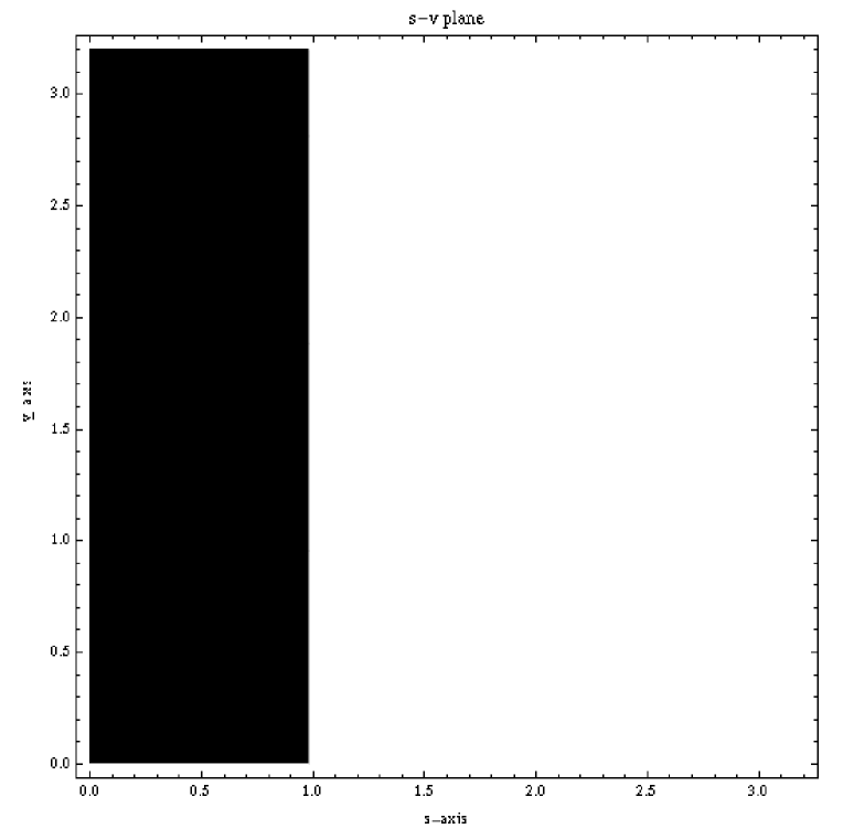
Figure 1: The stability region (s-v plane) of the classical Quinlan-Tremaine 12-step method

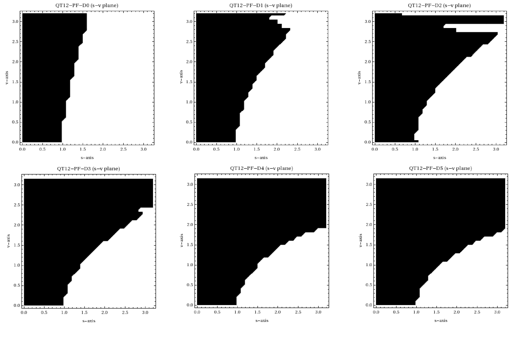
Figure 2: The stability region of the methods PF-D0,PF-D1, PF-D2, PF-D3, PF-D4 and PF-D5 (from left to right and from top to bottom)

The motivation of the above analysis is straightforward: Although the coefficients of the method (3) are designed in a way that the phase-lag and its first derivatives vanish in the frequency $\omega$, the frequency $\omega$ itself is unknown and only an estimation can be made. Thus, if the correct frequency of the problem is $\sigma$ we have to check if the method is stable, that is if the roots of the characteristic equation lie in the unit disk. For this reason we draw in the $s-v$ plane the areas in which the method is stable. Figure 1 shows the stability region for the classical method and figure 2 for the six methods (the phase fitted one and those with first,second, third, fourth and fifth phase lag derivative elimination). Note here that the $s$-axis corresponds to the real frequency while the $v$-axis corresponds to the estimated frequency used to construct the parameters of the method.

5 Numerical Results

The radial Schrödinger equation is given by:

$$y^{\prime\prime}(x)=\left(\frac{l(l+1)}{x^{2}}+V(x)-E)y(x)\right)$$ (23)

where $\frac{l(l+1)}{x^{2}}$ is the centrifugal potential, $V(x)$ is the potential, $E$ is the Energy and $W(x)=\frac{l(l+1)}{x^{2}}+V(x)$ is the effective potential. It is valid that $lim_{x\rightarrow\infty}V(x)=0$ and therefore $lim_{x\rightarrow\infty}W(x)=0$. We consider that $E>0$ and we divide the interval $[0,+\infty)$ into subintervals $[a_{i},b_{i}]$ so that $W(x)$ can be considered constant inside each subinterval with value $\hat{W}_{i}$. The problem (23) can be expressed now by the equations

$$y^{\prime\prime}_{i}=(\hat{W}_{i}-E)y_{i}$$ (24)

whose solution are

$$y_{i}(x)=\left(A_{i}e^{\sqrt{\hat{W}_{i}-E}x}+B_{i}e^{-\sqrt{\hat{W}_{i}-E}x}\right)$$ (25)

with $A_{i},B_{i}\in R$. We will integrate problem (23) with $l=0$ at the interval $[0,15]$ using the well known Woods-Saxon potential:

$$V(x)=\frac{u_{0}}{1+q}+\frac{U_{1}q}{(1+q)^{2}},\quad q=e^{\frac{x-x_{0}}{a}}$$ (26)

where $u_{0}=-50$, $a=0.6$, $x_{0}=7$, $u_{1}=-\frac{u_{0}}{a}$ and with boundary condition $y(0)=0$. The potential $V(x)$ decays more quickly than $\frac{l(l+1)}{x^{2}}$ , so for large x (asymptotic region) the Schrödinger equation (23) becomes

$$y^{\prime\prime}(x)=\left(\frac{l(l+1)}{x^{2}}-E)y(x)\right)$$ (27)

The last equation has two linearly independent solutions $kxj_{l}(kx)$ and $kxn_{l}(kx)$, where $j_{l}$ and $n_{l}$ are the spherical Bessel and Neumann functions and $k=\sqrt{\frac{l(l+1)}{x^{2}}-E}$. When $x\to\infty$ the solution takes the asymptotic form

$$y(x)\sim Akxj_{l}(kx)-Bkxn_{l}(kx)$$

$$\sim D[sin(kx-\pi\frac{l}{2})+tan(\delta_{l})\cos(kx-\pi\frac{l}{2})],$$ (28)

where $\delta_{l}$ is called the scattering phase shift and it is given by the following expression:

$$tan(\delta_{l})=\frac{y(x_{i})S(x_{i+1})-y(x_{i+1})S(x_{i})}{y(x_{i+1}C(x_{i})-y(x_{i})C(x_{i+1})}$$ (29)

where $S(x)=kxj_{l}(kx)$ and $C(x)=kxn_{l}(kx)$ and $x_{i}<x_{i+1}$ and both belong to the asymptotic region. Given the energy, we approximate the phase shift, the accurate value of which is $\frac{\pi}{2}$ for the above problem. We will use three different values for the energy: i) $989.701916$, ii) $341.495874$ and iii) $163.215341$. As for the frequency $\omega$ we will use the suggestion of Ixaru and Rizea [9]:

$$\omega=\left\{\begin{array}[]{ll}\sqrt{E-50},&x\in[0,6.5]\\ \sqrt{E},&x\in[6.5,15]\end{array}\right.$$ (30)

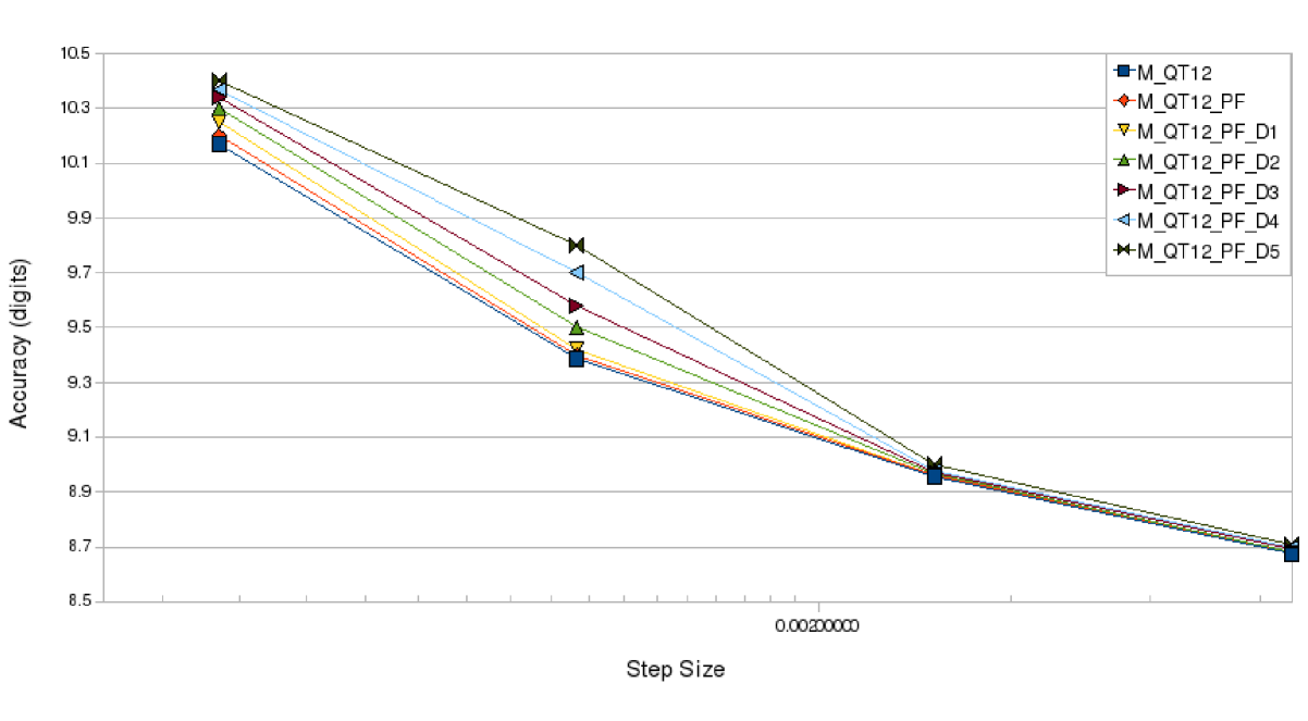
Figure 3: The accuracy (digits) of the new methods compared to the classical one for the Schrödinger equation ($E=989.701916$)

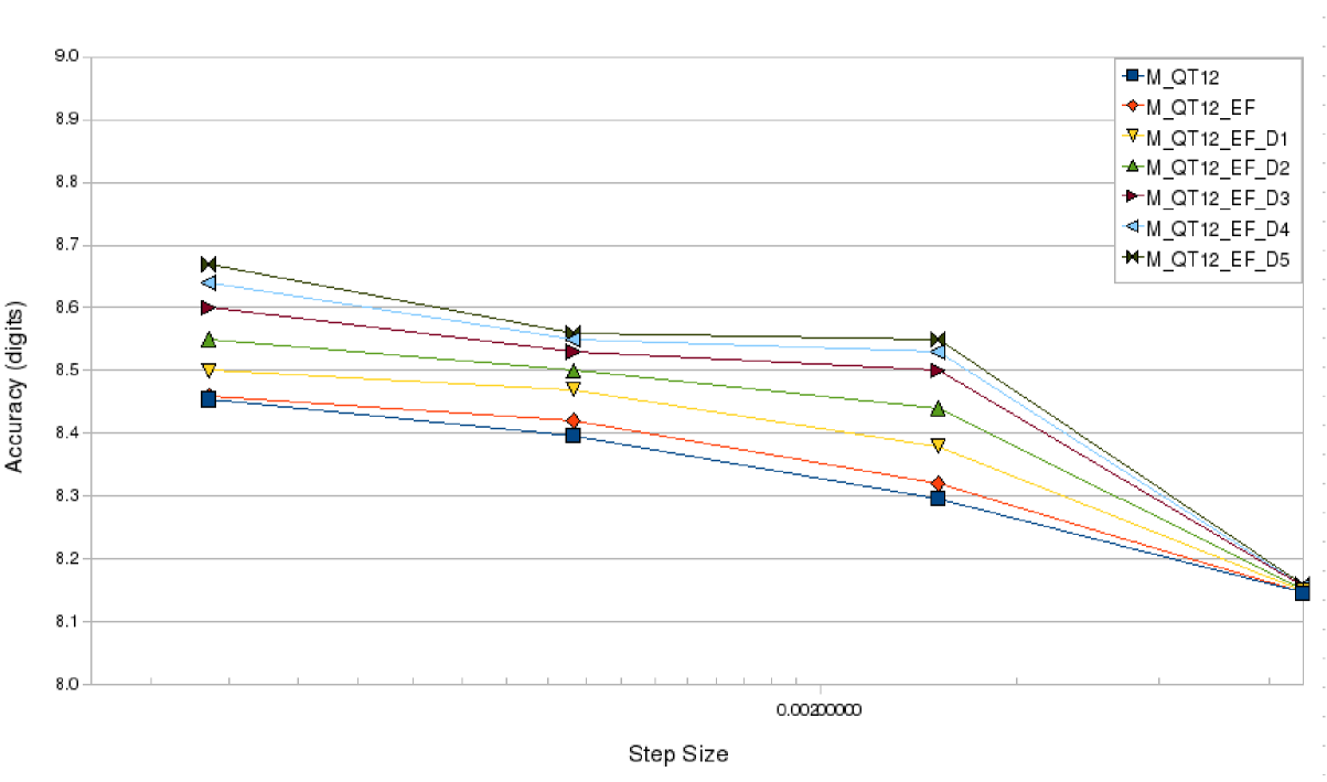
Figure 4: The accuracy (digits) of the new methods compared to the classical one for the Schrödinger equation ($E=341.495874$)

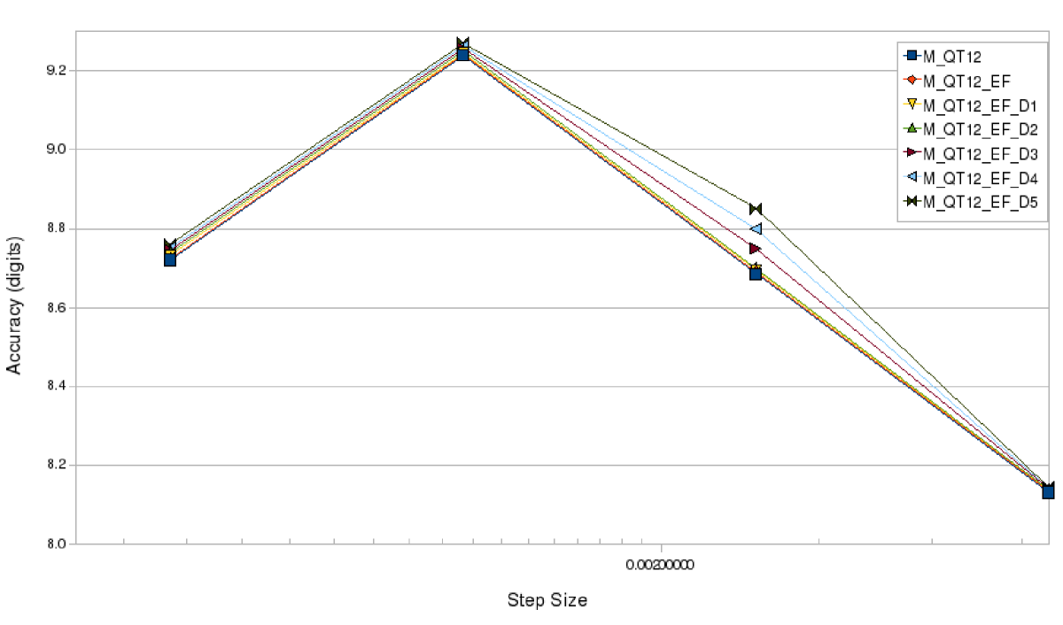
Figure 5: The accuracy (digits) of the new methods compared to the classical one for the Schrödinger equation ($E=163.215341$)

The results are shown in figures 3, 4 and 5. It is clear that the accuracy increases as the number of the eliminated derivatives of the phase lag function increases.

6 Conclusions

We have presented a new family of 12-step symmetric multistep numerical methods with improved characteristics concerning the integration of the Schrödinger equation. The methods were constructed by adopting a new methodology which, except for the phase fitting at a predefined frequency, it eliminates the first derivatives of the phase lag function at the same frequency. The result is that the phase lag function becomes less sensitive on the frequency near the predefined one. This behavior compensates the fact that the exact frequency can only be estimated. Experimental results demonstrate this behavior by showing that the accuracy is increased as the number of the derivatives that are eliminated is increased.

Method PF-D0:

$$\begin{array}[]{l}b_{1,num}^{0}=((-124184636\cos(v)+70378348\cos(2v)\\ -24862148\cos(3v)+5153611\cos(4v))v^{2}\\ +25(3013169v^{2}-16128\cos(3v)\\ +32256\cos(4v)-32256\cos(5v)+16128\cos(6v)))\csc^{10}(\frac{v}{2})\\ b_{2,num}^{0}=(v^{2}(159588050\cos(v)-85350160\cos(2v)\\ +16708985\cos(3v)-5153611\cos(5v))-16(6496079v^{2}\\ -252000\cos(3v)+504000\cos(4v)\\ -504000\cos(5v)+252000\cos(6v)))\csc^{10}(\frac{v}{2})\\ b_{3,num}^{0}=((-367257540\cos(v)+183567900\cos(2v)\\ -16708985\cos(4v)+24862148\cos(5v))v^{2}\\ +81(3175117v^{2}-224000\cos(3v)+448000\cos(4v)\\ -448000\cos(5v)+224000\cos(6v)))\csc^{10}(\frac{v}{2})\\ b_{4,num}^{0}=(30675810\cos(v)v^{2}-42958788v^{2}\\ +75(161280-611893v^{2})\cos(3v)\\ +140(152411v^{2}-172800)\cos(4v)\\ +(24192000-17594587v^{2})\cos(5v)-12096000\cos(6v))\csc^{10}(\frac{v}{2})\\ b_{5,num}^{0}=(-61351620\cos(2v)v^{2}+85936557v^{2}\\ +30(6120959v^{2}-1411200)\cos(3v)\\ +25(3386880-3191761v^{2})\cos(4v)\\ +(62092318v^{2}-84672000)\cos(5v)+42336000\cos(6v))\csc^{10}(\frac{v}{2})\\ b_{6,num}^{0}=((-171873114\cos(v)+171835152\cos(2v)\\ -257184477\cos(3v)+103937264\cos(4v)\\ -75329225\cos(5v))v^{2}+50803200(\cos(3v)-2\cos(4v)\\ +2\cos(5v)-\cos(6v)))\csc^{10}(\frac{v}{2})\\ b_{1,denom}^{0}=206438400v^{2}\\ b_{2,denom}^{0}=206438400v^{2}\\ b_{3,denom}^{0}=206438400v^{2}\\ b_{4,denom}^{0}=51609600v^{2}\\ b_{5,denom}^{0}=103219200v^{2}\\ b_{6,denom}^{0}=103219200v^{2}\end{array}$$

$$\begin{array}[]{l}\displaystyle b^{0}_{T,1}=\frac{90987349}{53222400}-\frac{16301796103\ v^{2}}{290594304000}+\frac{2012122579v^{4}}{581188608000}\\ \displaystyle-\frac{48410309\ v^{6}}{1184440320000}+\frac{991945331743\ v^{8}}{2838385676206080000}-\ldots\\ \displaystyle b^{0}_{T,2}=-\frac{114798419}{26611200}+\frac{16301796103\ v^{2}}{29059430400}-\frac{2012122579v^{4}}{58118860800}\\ \displaystyle+\frac{48410309\ v^{6}}{118444032000}-\frac{991945331743\ v^{8}}{283838567620608000}+\ldots\\ \displaystyle b^{0}_{T,3}=\frac{270875723}{17740800}-\frac{16301796103\ v^{2}}{6457651200}+\frac{2012122579v^{4}}{12915302400}\\ \displaystyle-\frac{48410309\ v^{6}}{26320896000}+\frac{991945331743\ v^{8}}{63075237249024000}-\ldots\\ \displaystyle b^{0}_{T,4}=-\frac{67855831}{2217600}+\frac{16301796103\ v^{2}}{2421619200}-\frac{2012122579v^{4}}{4843238400}\\ \displaystyle+\frac{48410309\ v^{6}}{9870336000}-\frac{991945331743\ v^{8}}{23653213968384000}+\ldots\\ \displaystyle b^{0}_{T,5}=\frac{50277247}{985600}-\frac{16301796103\ v^{2}}{1383782400}+\frac{2012122579v^{4}}{2767564800}\\ \displaystyle-\frac{48410309\ v^{6}}{5640192000}+\frac{991945331743\ v^{8}}{13516122267648000}-\ldots\\ \displaystyle b^{0}_{T,6}=-\frac{253491379}{4435200}+\frac{16301796103\ v^{2}}{1153152000}-\frac{2012122579v^{4}}{2306304000}\\ \displaystyle+\frac{48410309\ v^{6}}{4700160000}-\frac{991945331743\ v^{8}}{11263435223040000}+\ldots\\ \end{array}$$

Method PF-D1:

$$\begin{array}[]{l}b_{1,num}^{1}=\csc^{10}(\frac{v}{2})\sec(\frac{v}{2}\ )(53760(2\cos(v)+2\cos(2v)+2\cos(3v)\\ +2\cos(5\ v)+1)\sin^{3}(\frac{v}{2})+v((304823\cos\ (\frac{v}{2})-828603\cos(\frac{3v}{2})\\ +554639\cos(\frac{5v}{2})-272779\cos\ (\frac{7v}{2}))v^{2}+6720(7\cos(\frac{5\ v}{2})\\ -15\cos(\frac{7v}{2})+2(9\cos(\ \frac{9v}{2})-6\cos(\frac{11v}{2})+\cos\ (\frac{13v}{2})))))\\ b_{2,num}^{1}=\csc^{7}(\frac{v}{2})(v((393310\ \cos(2v)-211395\cos(3v)\\ +272779\cos(4v))v^{2}+(122851\ v^{2}+1088640)\cos(v)\\ -15(-1817v^{2}+74368\cos(2v)-65856\ \cos(3v)+45248\cos(4v)\\ -19040\cos(5v)+1344\cos(6v)+224\cos\ (7v)+36288))\csc^{3}(\frac{v}{2})\\ -26880(10\ \cos(v)+10\cos(2v)+9\cos(3v)+2\cos(4v)\\ +8\cos(5v)+\cos(6\ v)+5)\sec(\frac{v}{2}))\\ b_{3,num}^{1}=\csc^{7}(\frac{v}{2})(26880(90\cos\ (v)+90\cos(2v)+74\cos(3v)\\ +32\cos(4v)+58\cos(5v)+16\cos\ (6v)+45)\sec(\frac{v}{2})\\ -v((2519110\cos(2\ v)-654530\cos(3v)+272779(6\cos(4v)\\ +\cos(5v)))\ v^{2}+(1288471v^{2}+4717440)\cos(v)+8(47587\ v^{2}\\ -643440\cos(2v)+593880\cos(3v)-416640\cos(4v)\\ +159600\cos\ (5v)+18480\cos(6v)\\ -6720\cos(7v)-294840))\csc\ ^{3}(\frac{v}{2}))\\ b_{4,num}^{1}=\csc^{7}(\frac{v}{2})(v(1578002\ v^{2}+2(161489v^{2}+725760)\cos(v)\\ +160(20521\ v^{2}-13776)\cos(2v)+5(478464-4069v^{2})\cos(3\ v)\\ +2(738791v^{2}-900480)\cos(4v)+3(205341\ v^{2}+156800)\cos(5v)\\ +510720\cos(6v)-94080\cos(7\ v)-725760)\csc^{3}(\frac{v}{2})\\ -107520(30\cos\ (v)+30\cos(2v)+23\cos(3v)+14\cos(4v)\\ +16\cos(5v)+7\cos(6\ v)+15)\sec(\frac{v}{2}))\\ b_{5,num}^{1}=-\csc^{7}(\frac{v}{2})(v(923342\ v^{2}+28(343339v^{2}-181440)\cos(v)\\ +20(240593\ v^{2}+103488)\cos(2v)+5(832859v^{2}+18816)\cos(3\ v)\\ +2(1574159v^{2}-376320)\cos(4v)+3(913431\ v^{2}-313600)\cos(5v)\\ +2446080\cos(6v)-376320\cos(7\ v)+2540160)\csc^{3}(\frac{v}{2})\\ -376320(30\cos\ (v)+30\cos(2v)+22\cos(3v)+16\cos(4v)\\ +14\cos(5v)+8\cos(6\ v)+15)\sec(\frac{v}{2}))\\ b_{6,num}^{1}=\csc^{7}(\frac{v}{2})(v(7\ (65953v^{2}+181440)+7(379709v^{2}\\ -362880)\cos\ (v)+2(694753v^{2}+799680)\cos(2v)+4(360653\ v^{2}\\ -199920)\cos(3v)+15(52889v^{2}+21952)\cos(4\ v)\\ +(875393v^{2}-540960)\cos(5v)+799680\cos(6v)\\ -117600\ \cos(7v))\csc^{3}(\frac{v}{2})-188160(18\cos\ (v)+18\cos(2v)\\ +13\cos(3v)+10\cos(4v)+8\cos(5v)+5\cos(6\ v)+9)\sec(\frac{v}{2}))\\ b_{1,denom}^{1}=6881280v^{3}\\ b_{2,denom}^{1}=1720320v^{3}\\ b_{3,denom}^{1}=3440640v^{3}\\ b_{4,denom}^{1}=1720320v^{3}\\ b_{5,denom}^{1}=3440640v^{3}\\ b_{6,denom}^{1}=860160v^{3}\end{array}$$

$$\begin{array}[]{l}\displaystyle b^{1}_{T,1}=\frac{90987349}{53222400}-\frac{16301796103\ v^{2}}{145297152000}+\frac{1532031563\ v^{4}}{268240896000}\\ \displaystyle-\frac{31987133939\ v^{6}}{592812380160000}+\frac{5466168990203\ v^{8}}{2838385676206080000}+\ldots\\ \displaystyle b^{1}_{T,2}=-\frac{114798419}{26611200}+\frac{16301796103\ v^{2}}{14529715200}-\frac{28198975459\ v^{4}}{249080832000}\\ \displaystyle+\frac{88492028011\ v^{6}}{11856247603200}-\frac{533071354889581v^{8}}{1419192838103040000}+\ldots\\ \displaystyle b^{1}_{T,3}=\frac{270875723}{17740800}-\frac{16301796103\ v^{2}}{3228825600}+\frac{117200518583\ v^{4}}{166053888000}\\ \displaystyle-\frac{2285150767769\ v^{6}}{39520825344000}+\frac{308808361613933\ v^{8}}{105125395415040000}-\ldots\\ \displaystyle b^{1}_{T,4}=-\frac{67855831}{2217600}+\frac{16301796103\ v^{2}}{1210809600}-\frac{36423021893\ v^{4}}{16144128000}\\ \displaystyle+\frac{989757481543\ v^{6}}{4940103168000}-\frac{1207392034807669\ v^{8}}{118266069841920000}\ldots\\ \displaystyle b^{1}_{T,5}=\frac{50277247}{985600}-\frac{16301796103\ v^{2}}{691891200}+\frac{360410789243\ v^{4}}{83026944000}\\ \displaystyle-\frac{25035151487\ v^{6}}{62731468800}+\frac{125088382253381\ v^{8}}{6143691939840000}-\frac{2919882783787129\ v^{10}}{4460320348323840000}\ldots\\ \displaystyle b^{1}_{T,6}=-\frac{253491379}{4435200}+\frac{16301796103\ v^{2}}{576576000}-\frac{222767191987\ v^{4}}{41513472000}\\ \displaystyle+\frac{3516569786117\ v^{6}}{7057290240000}-\frac{95477706318691\ v^{8}}{3754478407680000}+\ldots\\ \end{array}$$

Method PF-D2:

$$\begin{array}[]{l}b_{1,num}^{2}=-30720(v^{2}-1)\cos(v)-10(-387\csc\ ^{6}(\frac{v}{2})\\ +72(128\cos(v)+127)\csc^{2}(v)+2048\ (v^{2}-3))-(8(-47v^{4}\\ -2040v^{2}-(40\ ((22\cos(v)+22\cos(2v)+9\cos(3v)+14\cos(4v)\\ +8\cos(5\ v)-5\cos(6v)+11)\tan^{3}(\frac{v}{2})-27v^{3})v)/(\ \cos(v)-1)\\ +(4817v^{4}+3120v^{2}\\ +4410)\cos(v)-2205\cos(2\ v)-2205))/((\cos(v)-1)^{4})\\ b_{2,num}^{2}=-1350v^{4}\csc^{10}(\frac{v}{2})+225v^{2}\ (59v^{2}+12)\csc^{8}(\frac{v}{2})\\ -5(7361\ v^{4}+3696v^{2}-540)\csc^{6}(\frac{v}{2})+6(4817\ v^{4}+3120v^{2}\\ -7710)\csc^{4}(\frac{v}{2})+264780\csc\ ^{2}(\frac{v}{2})+30720(3v^{2}-7)\cos(v)\\ +15360\ (v^{2}-2)\cos(2v)+30v\cot(\frac{v}{2})\ (\frac{1}{8}(-2436\cos(v)\\ +1921\cos(2v)+1595)\csc^{6}(\ \frac{v}{2})+8322)+10(5632v^{2}\\ -1024(8\cos(v)+23)\ \sin(v)v\\ \displaystyle+\frac{6(65\cos(v)+66)\tan(\frac{v}{2})v}{\ \cos(v)+1}-\frac{36}{\cos(v)+1}-39936)\\ b_{3,num}^{2}=12150v^{4}\csc^{10}(\frac{v}{2})-675v^{2}\ (191v^{2}+36)\csc^{8}(\frac{v}{2})\\ +15\ (28499v^{4}+12432v^{2}-1620)\csc^{6}(\frac{v}{2})-36450v\cot(\frac{v}{2})\csc^{6}(\frac{v}{2})\\ -12(44896v^{4}+26400v^{2}-35955)\csc\ ^{4}(\frac{v}{2})\\ +381960v\cot(\frac{v}{2})\ \csc^{4}(\frac{v}{2})+12(19268v^{4}+12480v^{2}\\ -219885)\csc^{2}(\frac{v}{2})-817950v\cot(\frac{v}{2}\ )\csc^{2}(\frac{v}{2})-540\sec^{2}(\frac{v}{2})\\ -5120(73v^{2}-831)-61440(9v^{2}-40)\cos\ (v)\\ -61440(3v^{2}-8)\cos(2v)-10240(v^{2}-3)\ \cos(3v)\\ -1512900v\cot(\frac{v}{2})+1884160v\sin\ (v)+532480v\sin(2v)\\ +30720v\sin(3v)+90v\sec\ ^{2}(\frac{v}{2})\tan(\frac{v}{2})+7740v\tan\ (\frac{v}{2})\\ b_{4,num}^{2}=-4050v^{4}\csc^{10}(\frac{v}{2})+675v^{2}\ (67v^{2}+12)\csc^{8}(\frac{v}{2})\\ -15(11113\ v^{4}+4464v^{2}-540)\csc^{6}(\frac{v}{2})+12150v\cot\ (\frac{v}{2})\csc^{6}(\frac{v}{2})\\ +6\ (43259v^{4}+24000v^{2}-24570)\csc^{4}(\frac{v}{2})-133920v\cot(\frac{v}{2})\csc^{4}(\frac{v}{2}\ )\\ +347250v\cot(\frac{v}{2})\csc\ ^{2}(\frac{v}{2})+8(4817v^{4}+15840v^{2}-197280)\\ +7680(19v^{2}-125)\cos(v)+30720(2v^{2}-7)\cos(2v)\\ +7680(v^{2}-3)\cos(3v)+292500v\cot\ (\frac{v}{2})-555520v\sin(v)\\ -194560v\sin(2v)-23040\ v\sin(3v)-30v\sec^{2}(\frac{v}{2})\tan\ (\frac{v}{2})\\ \displaystyle-3180v\tan(\frac{v}{2})+\frac{72(4817v^{4}+3120v^{2}-26165)}{\cos\ (v)-1}+\frac{360}{\cos(v)+1}\\ b_{5,num}^{2}=28350v^{4}\csc^{10}(\frac{v}{2})-14175v^{2}\ (23v^{2}+4)\csc^{8}(\frac{v}{2})\\ +45(28269\ v^{4}+10864v^{2}-1260)\csc^{6}(\frac{v}{2})-85050v\ \cot(\frac{v}{2})\csc^{6}(\frac{v}{2})\\ -12\ (182576v^{4}+98160v^{2}-87255)\csc^{4}(\frac{v}{2})\\ +965160v\cot(\frac{v}{2})\csc^{4}(\frac{v}{2}\ )+180(9634v^{4}+6240v^{2}\\ -38111)\csc\ ^{2}(\frac{v}{2})-2753430v\cot(\frac{v}{2})\ \csc^{2}(\frac{v}{2})-256(2011v^{4}\\ +3870v^{2}-45810)-15360(61v^{2}-479)\cos(v)-30720(13v^{2}\\ -56)\cos(2v)-76800(v^{2}-3)\cos(3v)-1054260v\cot\ (\frac{v}{2})\\ +3537920v\sin(v)+1372160v\sin(2\ v)+230400v\sin(3v)\\ \displaystyle-30v\sec^{2}(\frac{v}{2})\tan\ (\frac{v}{2})-2100v\tan(\frac{v}{2})+\frac{360}{\cos(v)+1}\end{array}$$

$$\begin{array}[]{l}b_{6,num}^{2}=93048v^{4}+156160v^{2}+1042425\csc^{2}(\frac{v}{2})\\ +15360(9v^{2}-74)\cos(v)-268800\cos(2v)-38400\ \cos(3v)\\ -(9(7560\csc^{2}(\frac{v}{2})+14963)v^{4}+187840v^{2}-4(237663v^{4}+77080v^{2}\\ +298620)\cos\ (v)+5((34095v^{4}-4000v^{2}+63126)\cos(2v)\\ -2v\ (v(14451v^{2}-5200)\cos(3v)+8(5v(140\cos(4\ v)-16\cos(5v)\\ -7\cos(6v)+2\cos(7v))-666\sin(v)+600\sin(2\ v)-298\sin(3v)\\ +238\sin(4v)+40\sin(5v)+80\sin(6v)-30\sin\ (7v))\\ +36(\sec^{2}(\frac{v}{2})+94)\tan(\ \frac{v}{2})))\\ \displaystyle+878850)/((\cos\ (v)-1)^{4})-\frac{270}{\cos(v)+1}-1793280\\ b_{1,denom}^{2}=5120v^{4}\\ b_{2,denom}^{2}=2560v^{4}\\ b_{3,denom}^{2}=5120v^{4}\\ b_{4,denom}^{2}=640v^{4}\\ b_{5,denom}^{2}=2560v^{4}\\ b_{6,denom}^{2}=320v^{4}\end{array}$$

$$\begin{array}[]{l}\displaystyle b^{2}_{T,1}=\frac{90987349}{53222400}-\frac{16301796103\ v^{2}}{96864768000}+\frac{1568734969\ v^{4}}{232475443200}\\ \displaystyle-\frac{112423833619\ v^{6}}{889218570240000}-\frac{128168340031\ v^{8}}{189225711747072000}-\ldots\\ \displaystyle b^{2}_{T,2}=-\frac{114798419}{26611200}+\frac{16301796103\ v^{2}}{9686476800}-\frac{10540703911\ v^{4}}{44706816000}\\ \displaystyle+\frac{871935134531\ v^{6}}{44460928512000}-\frac{463103326062011\ v^{8}}{473064279367680000}+\ldots\\ \displaystyle b^{2}_{T,3}=\frac{270875723}{17740800}-\frac{16301796103\ v^{2}}{2152550400}+\frac{639312597971\ v^{4}}{387459072000}\\ \displaystyle-\frac{2472777112313\ v^{6}}{11856247603200}+\frac{58110459403753\ v^{8}}{3185618042880000}-\ldots\\ \displaystyle b^{2}_{T,4}=-\frac{67855831}{2217600}+\frac{16301796103\ v^{2}}{807206400}-\frac{89147839889\ v^{4}}{16144128000}\\ \displaystyle+\frac{1282661397349\ v^{6}}{1482030950400}-\frac{3541527647083319\ v^{8}}{39422023280640000}+\ldots\\ \displaystyle b^{2}_{T,5}=\frac{50277247}{985600}-\frac{16301796103\ v^{2}}{461260800}+\frac{300047111873\ v^{4}}{27675648000}\\ \displaystyle-\frac{18727460555953\ v^{6}}{9880206336000}+\frac{4749826752625121\ v^{8}}{22526870446080000}-\ldots\\ \displaystyle b^{2}_{T,6}=-\frac{253491379}{4435200}+\frac{16301796103\ v^{2}}{384384000}-\frac{37309797113\ v^{4}}{2767564800}\\ \displaystyle+\frac{90333884682737\ v^{6}}{37050773760000}-\frac{69221174089601\ v^{8}}{250298560512000}+\ldots\end{array}$$

Method PF-D3:

$$\begin{array}[]{l}b_{1,num}^{3}=-108v^{5}\csc^{10}(\frac{v}{2})+9v^{3}\ (53v^{2}+12)\csc^{8}(\frac{v}{2})\\ +486v\csc\ ^{6}(\frac{v}{2})-2484v\csc^{4}(\frac{v}{2})-6144v(4v^{2}-9)\cos(v)\\ +3\cot(\frac{v}{2})(99v^{2}\csc^{6}(\frac{v}{2})+9(16-9v^{2})\csc^{4}(\frac{v}{2})-8(113v^{2}\\ +276)\csc\ ^{2}(\frac{v}{2})-11266v^{2}+10032)-6144(v^{3}-6\ v+4\sin(v))\\ +2v^{2}(26624\sin(v)-5635\tan\ (\frac{v}{2}))+5520\tan(\frac{v}{2})\\ -9\ v\sec^{4}(\frac{v}{2})(v\tan(\frac{v}{2})-6)-6\sec^{2}(\frac{v}{2})((61\ v^{2}+24)\tan(\frac{v}{2})\\ \displaystyle-363v)+\frac{32508\ v}{\cos(v)-1}\\ b_{2,num}^{3}=540v^{5}\csc^{10}(\frac{v}{2})-45v^{3}\ (71v^{2}+12)\csc^{8}(\frac{v}{2})\\ +18v(212\ v^{4}+48v^{2}-135)\csc^{6}(\frac{v}{2})-1485v^{2}\cot\ (\frac{v}{2})\csc^{6}(\frac{v}{2})\\ +15984v\csc\ ^{4}(\frac{v}{2})+27(131v^{2}-80)\cot\ (\frac{v}{2})\csc^{4}(\frac{v}{2})\\ +55782v\csc\ ^{2}(\frac{v}{2})+6(1777v^{2}+5952)\cot\ (\frac{v}{2})\csc^{2}(\frac{v}{2})\\ +54v\sec^{4}\ (\frac{v}{2})+6144v(5v^{2}-39)+6144v(8\ v^{2}-33)\cos(v)\\ +18432v(v^{2}-4)\cos(2v)+6\ (20035v^{2}-31704)\cot(\frac{v}{2})\\ -20480\ (7v^{2}-6)\sin(v)+3072(12-19v^{2})\sin(2\ v)\\ -9v^{2}\sec^{4}(\frac{v}{2})\tan(\frac{v}{2})-12(23v^{2}+12)\sec^{2}(\frac{v}{2})\tan\ (\frac{v}{2})\\ \displaystyle+14(456-337v^{2})\tan\ (\frac{v}{2})+\frac{3276v}{\cos(v)+1}\\ b_{3,num}^{3}=-1620v^{5}\csc^{10}(\frac{v}{2})+135v^{3}\ (85v^{2}+12)\csc^{8}(\frac{v}{2})\\ -6v(3872\ v^{4}+768v^{2}-1215)\csc^{6}(\frac{v}{2})+4455v^{2}\cot\ (\frac{v}{2})\csc^{6}(\frac{v}{2})\\ +36v\ (424v^{4}+96v^{2}-1563)\csc^{4}(\frac{v}{2})+9\ (720\\ -1781v^{2})\cot(\frac{v}{2})\csc^{4}(\ \frac{v}{2})-96642v\csc^{2}(\frac{v}{2})-24\ (685v^{2}\\ +4716)\cot(\frac{v}{2})\csc^{2}(\ \frac{v}{2})-54v\sec^{4}(\frac{v}{2})+1024v\ (606-67v^{2})\\ -49152v(2v^{2}-13)\cos(v)-49152\ v(v^{2}-5)\cos(2v)\\ +2048v(21-4v^{2})\cos(3\ v)+6(111720-46199v^{2})\cot(\frac{v}{2})\\ +32768(11v^{2}-15)\sin(v)+4096(41v^{2}-36)\sin(2v)\\ +4096(7v^{2}-6)\sin(3v)+9v^{2}\sec\ ^{4}(\frac{v}{2})\tan(\frac{v}{2})+6(61\ v^{2}\\ \displaystyle+24)\sec^{2}(\frac{v}{2})\tan(\frac{v}{2})+10(1055v^{2}-552)\tan(\frac{v}{2})-\frac{4356v}{\cos(v)+1}\\ b_{4,num}^{3}=1620v^{5}\csc^{10}(\frac{v}{2})-135v^{3}\ (95v^{2}+12)\csc^{8}(\frac{v}{2})\\ +18v\ (1844v^{4}+336v^{2}-405)\csc^{6}(\frac{v}{2})-4455v^{2}\cot(\frac{v}{2})\csc^{6}(\frac{v}{2}\ )\\ -216v(169v^{4}+36v^{2}-288)\csc\ ^{4}(\frac{v}{2})+27(737v^{2}\\ -240)\cot\ (\frac{v}{2})\csc^{4}(\frac{v}{2})+18v\ (848v^{4}+192v^{2}+2229)\csc^{2}(\frac{v}{2})\\ +18\ (35v^{2}+6528)\cot(\frac{v}{2})\csc\ ^{2}(\frac{v}{2})-54v\sec^{4}(\frac{v}{2})+384v\ (133v^{2}\\ -1350)+768v(112v^{2}-843)\cos\ (v)+3072v(13v^{2}-81)\cos(2v)\\ +1536v(8v^{2}-45)\cos(3v)+768v(v^{2}-6)\cos(4v)+54(4447\ v^{2}\\ -13800)\cot(\frac{v}{2})+512(1146-659v^{2}\ )\sin(v)-512(289v^{2}\\ -348)\sin(2v)+1024\ (42-43v^{2})\sin(3v)+256(12\\ \displaystyle-11v^{2})\sin(4\ v)+(9v^{2}\sec^{4}(\frac{v}{2})+5258v^{2}+\frac{552\ v^{2}+288}{\cos(v)+1}\\ \displaystyle-6384)\tan(\frac{v}{2})-\frac{3276v}{\cos(v)+1}\end{array}$$

$$\begin{array}[]{l}b_{5,num}^{3}=-11340v^{5}\csc^{10}(\frac{v}{2})+945v^{3}\ (101v^{2}+12)\csc^{8}(\frac{v}{2})\\ -18v\ (15472v^{4}+2688v^{2}-2835)\csc^{6}(\frac{v}{2})\\ +31185v^{2}\cot(\frac{v}{2})\csc\ ^{6}(\frac{v}{2})+108v(3500v^{4}+720v^{2}-4263)\ \csc^{4}(\frac{v}{2})\\ +189(240-823v^{2})\cot\ (\frac{v}{2})\csc^{4}(\frac{v}{2})+864(87\ v^{2}\\ -973)\cot(\frac{v}{2})\csc^{2}(\frac{v}{2}\ )+54v\sec^{4}(\frac{v}{2})+384v(159v^{4}-796\ v^{2}\\ +8568)+3072v(1395-172v^{2})\cos(v)-24576v\ (11v^{2}\\ -75)\cos(2v)+3072v(171-28v^{2})\cos\ (3v)\\ -12288v(v^{2}-6)\cos(4v)+18(307848-88943v^{2}\ )\cot(\frac{v}{2})\\ +2048(1055v^{2}-2154)\ \sin(v)+2048(505v^{2}-708)\sin(2v)\\ +2048(155\ v^{2}-174)\sin(3v)+4096(11v^{2}-12)\sin(4v)\\ -9\ v^{2}\sec^{4}(\frac{v}{2})\tan(\frac{v}{2})-6\ (61v^{2}+24)\sec^{2}(\frac{v}{2})\tan\ (\frac{v}{2})+10(552\\ \displaystyle-1019v^{2})\tan\ (\frac{v}{2})+\frac{36v(256(53v^{2}+12)\ v^{2}+1479)}{\cos(v)-1}+\frac{4356v}{\cos(v)+1}\\ b_{6,num}^{3}=2268v^{5}\csc^{10}(\frac{v}{2})-189v^{3}\ (103v^{2}+12)\csc^{8}(\frac{v}{2})\\ +6v\ (9820v^{4}+1680v^{2}-1701)\csc^{6}(\frac{v}{2})-6237v^{2}\cot(\frac{v}{2})\csc^{6}(\frac{v}{2}\ )\\ -144v(590v^{4}+120v^{2}-651)\csc\ ^{4}(\frac{v}{2})+63(511v^{2}\\ -144)\cot\ (\frac{v}{2})\csc^{4}(\frac{v}{2})+18v\ (3392v^{4}+768v^{2}-677)\csc^{2}(\frac{v}{2})\\ +6\ (28224-3463v^{2})\cot(\frac{v}{2})\csc\ ^{2}(\frac{v}{2})+54v\sec^{4}(\frac{v}{2})\\ -128v\ (141v^{4}-460v^{2}+5016)+3072v(32v^{2}-269)\cos\ (v)\\ +6144v(9v^{2}-62)\cos(2v)+2048v(8v^{2}-51)\cos(3v)\\ +3072v(v^{2}-6)\cos(4v)+1002(317\ v^{2}-1128)\cot(\frac{v}{2})\\ -6144(67v^{2}-146)\sin(v)-3072(69v^{2}-100)\sin(2v)\\ -12288(5\ v^{2}-6)\sin(3v)+1024(12-11v^{2})\sin(4\ v)\\ \displaystyle-(9v^{2}\sec^{4}(\frac{v}{2})+5438v^{2}+\frac{552\ v^{2}+288}{\cos(v)+1}-6384)\tan(\frac{v}{2})\\ \displaystyle+\frac{3276v}{\cos(v)+1}\\ b_{1,denom}^{3}=3072v^{5}\\ b_{2,denom}^{3}=1536v^{5}\\ b_{3,denom}^{3}=1024v^{5}\\ b_{4,denom}^{3}=384v^{5}\\ b_{5,denom}^{3}=1536v^{5}\\ b_{6,denom}^{3}=256v^{5}\end{array}$$

$$\begin{array}[]{l}\displaystyle b^{3}_{T,1}=\frac{90987349}{53222400}-\frac{16301796103\ v^{2}}{72648576000}+\frac{1273143229v^{4}}{193729536000}\\ \displaystyle-\frac{421960559\ v^{6}}{1221454080000}-\frac{124506164597657\ v^{8}}{5676771352412160000}-\ldots\\ \displaystyle b^{3}_{T,2}=-\frac{114798419}{26611200}+\frac{16301796103\ v^{2}}{7264857600}-\frac{38969308351v^{4}}{96864768000}\\ \displaystyle+\frac{5604849953\ v^{6}}{158789030400}-\frac{5242236508523657\ v^{8}}{2838385676206080000}+\ldots\\ \displaystyle b^{3}_{T,3}=\frac{270875723}{17740800}-\frac{16301796103\ v^{2}}{1614412800}+\frac{578948920601\ v^{4}}{193729536000}\\ \displaystyle-\frac{733132845253\ v^{6}}{1482030950400}+\frac{3064860132866873\ v^{8}}{57341124771840000}-\ldots\\ \displaystyle b^{3}_{T,4}=-\frac{67855831}{2217600}+\frac{16301796103\ v^{2}}{605404800}-\frac{247322293877\ v^{4}}{24216192000}\\ \displaystyle+\frac{844539338551\ v^{6}}{370507737600}-\frac{80127849554001773\ v^{8}}{236532139683840000}+\ldots\\ \displaystyle b^{3}_{T,5}=\frac{50277247}{985600}-\frac{16301796103\ v^{2}}{345945600}+\frac{279925886083\ v^{4}}{13837824000}\\ \displaystyle-\frac{644885438797\ v^{6}}{123502579200}+\frac{122198747647321067v^{8}}{135161222676480000}-\ldots\\ \displaystyle b^{3}_{T,6}=-\frac{253491379}{4435200}+\frac{16301796103\ v^{2}}{288288000}-\frac{1220113637v^{4}}{48384000}\\ \displaystyle+\frac{55089606671\ v^{6}}{8096760000}-\frac{1634963205351829\ v^{8}}{1325110026240000}+\ldots\\ \end{array}$$

Method PF-D4:

$$\begin{array}[]{l}b_{1,num}^{4}=216v^{6}\csc^{10}(\frac{v}{2})-810v^{2}\csc\ ^{6}(\frac{v}{2})-54(157v^{2}\\ +80)\csc\ ^{4}(\frac{v}{2})+36(1840-2257v^{2})\csc\ ^{2}(\frac{v}{2})-12288(20v^{4}\\ -71v^{2}+20)\cos\ (v)-3v\cot(\frac{v}{2})((4682v^{2}+9\csc\ ^{2}(\frac{v}{2})(5\csc^{2}(\frac{v}{2})\ v^{2}\\ +54v^{2}+96)+5856)\csc^{2}(\frac{v}{2})+2520\ (31v^{2}-48))\\ -45v^{2}\sec^{6}(\frac{v}{2})\ (v\tan(\frac{v}{2})-6)+56v(1024\ (11v^{2}-12)\sin(v)\\ +135(48-31v^{2})\tan\ (\frac{v}{2}))-18\sec^{4}(\frac{v}{2})\ (-373v^{2}+3(21v^{2}\\ +16)\tan(\frac{v}{2})\ v-80)-2\sec^{2}(\frac{v}{2})(-39246\ v^{2}\\ +(6733v^{2}+6384)\tan(\frac{v}{2})v+28320)\\ b_{2,num}^{4}=-1080v^{6}\csc^{10}(\frac{v}{2})+2160v^{6}\ \csc^{8}(\frac{v}{2})+4050v^{2}\csc^{6}(\frac{v}{2})\\ +54(617v^{2}+400)\csc^{4}(\frac{v}{2})+293508v^{2}\csc^{2}(\frac{v}{2})+12288(20\ v^{4}\\ -71v^{2}+20)\cos(v)+24576(10v^{4}-59v^{2}+20)\ \cos(2v)\\ +3v\cot(\frac{v}{2})((16978v^{2}+9\ \csc^{2}(\frac{v}{2})(25\csc^{2}(\frac{v}{2})v^{2}+214v^{2}+480)\\ +20064)\csc^{2}(\frac{v}{2})+120(2341v^{2}-5136))+(72(4096\ v^{4}\\ -31783v^{2}-80(257\cos(v)+251)\csc^{2}(v)+1024(4v^{4}-35\ v^{2}\\ +20)\cos(v)+25600))/(\cos(v)+1)-v(135v\ (v\tan(\frac{v}{2})\\ -6)\sec\ ^{6}(\frac{v}{2})+18((161v^{2}+144)\tan\ (\frac{v}{2})-951v)\sec^{4}(\frac{v}{2})\\ +18(1407v^{2}+1616)\tan(\frac{v}{2})\ \sec^{2}(\frac{v}{2})+8(7168(11v^{2}-12)\ \sin(v)\\ +1024(107v^{2}-156)\sin(2v)+15(3217\ v^{2}-9168)\tan(\frac{v}{2})))\\ b_{3,num}^{4}=9720v^{6}\csc^{10}(\frac{v}{2})-34560v^{6}\ \csc^{8}(\frac{v}{2})+270v^{2}(128v^{4}\\ -135)\csc\ ^{6}(\frac{v}{2})-6075v^{3}\cot(\frac{v}{2})\ \csc^{6}(\frac{v}{2})-162(1459v^{2}\\ +1200)\csc\ ^{4}(\frac{v}{2})-54v(767v^{2}+2160)\cot(\ \frac{v}{2})\csc^{4}(\frac{v}{2})\\ +108\ (32720-18831v^{2})\csc^{2}(\frac{v}{2})-234v\ (1511v^{2}\\ +1488)\cot(\frac{v}{2})\csc\ ^{2}(\frac{v}{2})+3510v^{2}\sec^{6}(\frac{v}{2})+90(701v^{2}\\ +208)\sec^{4}(\frac{v}{2})-12288(98v^{4}-825v^{2}+540)-12288(220v^{4}\\ -1717\ v^{2}+940)\cos(v)-98304(10v^{4}-59v^{2}+20)\cos(2\ v)\\ -24576(20v^{4}-147v^{2}+60)\cos(3v)+360v\ (45744\\ -16567v^{2})\cot(\frac{v}{2})+8192v\ (1279v^{2}-2868)\sin(v)+32768v(107v^{2}\\ -156)\ \sin(2v)+147456v(13v^{2}-24)\sin(3v)-v(585v^{2}\ \sec^{6}(\frac{v}{2})\\ +(42991v^{2}+(32281v^{2}+46128\ )\cos(v)+57360)\sec^{4}(\frac{v}{2})\\ \displaystyle+120\ (8741v^{2}-38928))\tan(\frac{v}{2})+\frac{24(30457v^{2}-69040)}{\cos(v)+1}\\ b_{4,num}^{4}=-3240v^{6}\csc^{10}(\frac{v}{2})+15120v^{6}\ \csc^{8}(\frac{v}{2})-810v^{2}(32v^{4}\\ -15)\csc\ ^{6}(\frac{v}{2})+2025v^{3}\cot(\frac{v}{2})\ \csc^{6}(\frac{v}{2})+54(320v^{6}+1179v^{2}\\ +1200)\ \csc^{4}(\frac{v}{2})+54v(209v^{2}+720)\cot\ (\frac{v}{2})\csc^{4}(\frac{v}{2})\\ +108\ (5237v^{2}-11440)\csc^{2}(\frac{v}{2})+18v\ (5461v^{2}\\ +3888)\cot(\frac{v}{2})\csc\ ^{2}(\frac{v}{2})+270v^{2}\sec^{6}(\frac{v}{2})+90\ (41v^{2}+16)\sec^{4}(\frac{v}{2})\\ +76800(5\ v^{4}-54v^{2}+48)+6144(100v^{4}-819v^{2}+480)\cos\ (v)\\ +73728(5v^{4}-39v^{2}+20)\cos(2v)+6144(20\ v^{4}-147v^{2}\\ +60)\cos(3v)+6144(5v^{4}-41v^{2}+20)\ \cos(4v)+360v(4705v^{2}\\ -14928)\cot(\frac{v}{2})-36864v(67v^{2}-154)\sin(v)-86016v(17\ v^{2}\\ -36)\sin(2v)-36864v(13v^{2}-24)\sin(3\ v)-2048v(61v^{2}\\ -132)\sin(4v)-v\ \displaystyle(((1087+\frac{90}{\cos(v)+1})v^{2}+(457\ v^{2}\\ \displaystyle+1776)\cos(v)+2640)\sec^{4}(\frac{v}{2})+120(349v^{2}\\ \displaystyle-2832))\tan(\frac{v}{2})+\frac{24(349v^{2}-5680)}{\cos(v)+1}\end{array}$$

$$\begin{array}[]{l}b_{5,num}^{4}=22680v^{6}\csc^{10}(\frac{v}{2})-120960v^{6}\ \csc^{8}(\frac{v}{2})+4050v^{2}(64v^{4}\\ -21)\csc\ ^{6}(\frac{v}{2})-14175v^{3}\cot(\frac{v}{2})\ \csc^{6}(\frac{v}{2})-54(5120v^{6}+7077v^{2}\\ +8400)\csc^{4}(\frac{v}{2})-378v(181v^{2}+720)\ \cot(\frac{v}{2})\csc^{4}(\frac{v}{2})+108\ (1280v^{6}\\ -33131v^{2}+82320)\csc^{2}(\frac{v}{2})-378v(1643v^{2}+784)\cot(\frac{v}{2})\ \csc^{2}(\frac{v}{2})\\ -1890v^{2}\sec^{6}(\frac{v}{2})-126(277v^{2}+80)\sec^{4}(\frac{v}{2})-15360(160v^{4}\\ -1833v^{2}+1740)-30720(120\ v^{4}-1079v^{2}+740)\cos(v)\\ -6144(400v^{4}-3271v^{2}+1780)\cos(2v)-6144(140v^{4}-1113v^{2}\\ +540)\cos(3\ v)-49152(5v^{4}-41v^{2}+20)\cos(4v)-6144(4v^{4}\\ -35\ v^{2}+20)\cos(5v)+360v(102576-30047v^{2})\cot\ (\frac{v}{2})\\ +20480v(755v^{2}-1956)\sin\ (v)+4096v(2429v^{2}-5412)\sin(2v)\\ +12288v(281\ v^{2}-588)\sin(3v)+16384v(61v^{2}-132)\sin(4\ v)\\ +20480v(5v^{2}-12)\sin(5v)+v\ (((25429+\frac{630}{\cos(v)+1})v^{2}+(19507\ v^{2}\\ \displaystyle+26256)\cos(v)+32304)\sec^{4}(\frac{v}{2})+120(5347v^{2}-20976))\tan(\frac{v}{2})\\ \displaystyle+\frac{885120-443976v^{2}}{\cos(v)+1}\\ b_{6,num}^{4}=-13608v^{6}\csc^{10}(\frac{v}{2})+75600v^{6}\ \csc^{8}(\frac{v}{2})+270v^{2}(189\\ -640v^{4})\csc\ ^{6}(\frac{v}{2})+8505v^{3}\cot(\frac{v}{2})\ \csc^{6}(\frac{v}{2})+162(1280v^{6}\\ +1337v^{2}+1680)\csc^{4}(\frac{v}{2})+378v(103v^{2}+432)\ \cot(\frac{v}{2})\csc^{4}(\frac{v}{2})\\ +126v\ (2863v^{2}+1104)\cot(\frac{v}{2})\csc\ ^{2}(\frac{v}{2})-1890v^{2}\sec^{6}(\frac{v}{2})\\ -126(253v^{2}+80)\sec^{4}(\frac{v}{2})+3072(18v^{6}+400v^{4}-4575v^{2}+4500)\\ +30720(80\ v^{4}-753v^{2}+540)\cos(v)+30720(40v^{4}-327v^{2}\\ +180)\ \cos(2v)+6144(100v^{4}-819v^{2}+420)\cos(3v)+24576\ (5v^{4}\\ -41v^{2}+20)\cos(4v)+6144(4v^{4}-35v^{2}+20)\cos(5v)\\ +360v(17495v^{2}-61104)\cot\ (\frac{v}{2})-552960v(19v^{2}-52)\sin\ (v)\\ -552960v(9v^{2}-20)\sin(2v)-12288v(203\ v^{2}-444)\sin(3v)\\ -8192v(61v^{2}-132)\sin(4\ v)-20480v(5v^{2}-12)\sin(5v)\\ +v(63(48\ (v^{2}+1)+(43v^{2}+48)\cos(v))\sec\ ^{6}(\frac{v}{2})+840(659v^{2}\\ \displaystyle-2928)+\frac{57964\ v^{2}+86592}{\cos(v)+1})\tan(\frac{v}{2})\\ \displaystyle+\frac{216\ (1280v^{6}-19257v^{2}+49840)}{\cos\ (v)-1}+\frac{908160-325608v^{2}}{\cos(v)+1}\\ b_{1,denom}^{4}=24576v^{6}\\ b_{2,denom}^{4}=12288v^{6}\\ b_{3,denom}^{4}=24576v^{6}\\ b_{4,denom}^{4}=3072v^{6}\\ b_{5,denom}^{4}=12288v^{6}\\ b_{6,denom}^{4}=6144v^{6}\end{array}$$

$$\begin{array}[]{l}\displaystyle b^{4}_{T,1}=\frac{90987349}{53222400}-\frac{16301796103\ v^{2}}{58118860800}+\frac{451826777\ v^{4}}{87178291200}\\ \displaystyle-\frac{567827928197\ v^{6}}{711374856192000}-\frac{7456559915267\ v^{8}}{87334943883264000}-\ldots\\ \displaystyle b^{4}_{T,2}=-\frac{114798419}{26611200}+\frac{16301796103\ v^{2}}{5811886080}-\frac{53423656079\ v^{4}}{87178291200}+\\ \displaystyle\frac{3768047264957\ v^{6}}{71137485619200}-\frac{1807362562020419v^{8}}{567677135241216000}+\ldots\\ \displaystyle b^{4}_{T,3}=\frac{270875723}{17740800}-\frac{16301796103\ v^{2}}{1291530240}+\frac{137191770479\ v^{4}}{29059430400}\\ \displaystyle-\frac{6482264498201\ v^{6}}{6774998630400}+\frac{177746918811101\ v^{8}}{1557413265408000}-\ldots\\ \displaystyle b^{4}_{T,4}=-\frac{67855831}{2217600}+\frac{16301796103\ v^{2}}{484323840}-\frac{4393734833v^{4}}{269068800}\\ \displaystyle+\frac{3998343544387\ v^{6}}{846874828800}-\frac{42449166474915191\ v^{8}}{47306427936768000}+\ldots\\ \displaystyle b^{4}_{T,5}=\frac{50277247}{985600}-\frac{16301796103\ v^{2}}{276756480}+\frac{9638045471v^{4}}{296524800}\\ \displaystyle-\frac{87748735805873\ v^{6}}{7904165068800}+\frac{70694795981650949\ v^{8}}{27032244535296000}-\ldots\\ \displaystyle b^{4}_{T,6}=-\frac{253491379}{4435200}+\frac{16301796103\ v^{2}}{230630400}-\frac{84219941177\ v^{4}}{2075673600}\\ \displaystyle+\frac{863717128805537\ v^{6}}{59281238016000}-\frac{1830923526668191\ v^{8}}{500597121024000}+\ldots\end{array}$$

Method PF-D5:

$$\begin{array}[]{l}b_{1,num}^{5}=-\cos^{5}(\frac{v}{2})\csc^{13}(v)\sin\ ^{7}(\frac{v}{2})(60(-5v^{5}+3v^{3}+3\sin(v)\\ -6\ \sin(3v)+3\sin(4v)+3\sin(5v)-6\sin(6v)+3\sin(8v))\\ +\frac{1}{2}v(15(200v^{4}+283v^{2}-100)\cos\ (v)+300(2\cos(2v)+6\cos(3v)\\ -10\cos(4v)+\cos(5v)+12\cos\ (6v)-2\cos(7v)-4\cos(8v))\\ +v(v(15(366\cos(3\ v)+686\cos(4v)-503\cos(5v)-480\cos(6v)\\ +142\cos(7v)+116\ \cos(8v))+2(15(72v^{2}-155)\cos(2v)\\ +v(-60\ v(45\cos(3v)+24\cos(4v)-25\cos(5v)-14\cos(6v)\\ +5\cos(7\ v)+3\cos(8v))+405\cot(\frac{v}{2})+357\sin(v)-2530\ \sin(2v)\\ +4516\sin(3v)+3752\sin(4v)-3373\sin(5v)-2324\sin\ (6v)\\ +770\sin(7v)+522\sin(8v)+315\tan(\frac{v}{2})\ )))-60(49\sin(v)\\ -44\sin(2v)-6\sin(3v)+131\ \sin(4v)-67\sin(5v)-114\sin(6v)\\ +28\sin(7v)+31\sin(8v)))))\\ b_{2,num}^{5}=\csc^{7}(\frac{v}{2})\sec^{9}(\frac{v}{2})(4(3875v^{4}-519v^{2}-90)\cos(v)\\ -36(147\ v^{4}-76v^{2}-10\cos(2v)+20\cos(4v)-20\cos(5v)\\ +10\cos(7v)-20\ \cos(8v)+10\cos(10v))+v(v(2(5117\ v^{2}\\ -4254)\cos(2v)+12(516\cos(3v)+482\cos(4v)-158\cos\ (5v)\\ +348\cos(6v)-317\cos(7v)-486\cos(8v)+132\cos(9v)\\ +137\ \cos(10v))+v(3(-12\sin(v)-3789\sin(2v)+3900\sin(3\ v)\\ +2058\sin(4v)+708\sin(5v)+1632\sin(6v)-2142\sin(7\ v)\\ -1792\sin(8v)+614\sin(9v)+461\sin(10v))\\ -2v(-393216\ v(15\cos(2v)+17)\sin^{7}(\frac{v}{2})\cos\ ^{9}(\frac{v}{2})+4476\cos(3v)\\ +1918\cos(4v)+2288\cos\ (5v)+1242\cos(6v)-2476\cos(7v)\\ -1400\cos(8v)+582\cos(9\ v)+351\cos(10v))))\\ -15360\cos\ ^{3}(\frac{v}{2})(186\cos(v)+156\cos(2v)+132\cos(3\ v)\\ +78\cos(4v)+48\cos(5v)+19\cos(6v)+98)\sin\ ^{5}(\frac{v}{2})))\\ b_{3,num}^{5}=-\cos^{6}(\frac{v}{2})\csc^{14}(v)\sin\ ^{8}(\frac{v}{2})(7290\cot(\frac{v}{2})\ v^{4}\\ +5670\tan(\frac{v}{2})v^{4}+32(56v^{2}-93)\ \sin(9v)v^{2}+12(250v^{4}-751v^{2}\\ +100)v+3(2140\ v^{4}+13737v^{2}-2220)\cos(v)v-6(260v^{4}\\ -591v^{2}+540)\cos(2v)v+6(-1702v^{4}+2971v^{2}+1100)\cos(3v)\ v\\ -6(584v^{4}-3933v^{2}+1020)\cos(4v)v+15(236\ v^{4}-1395v^{2}\\ +228)\cos(5v)v+12(182v^{4}-1121v^{2}+800)\cos(6v)v+12(61v^{4}\\ -201v^{2}-180)\cos(7v)v+12\ (10v^{4}-171v^{2}+60)\cos(8v)v\\ -60(8v^{4}-53v^{2}+20)\cos(9v)v-24(10v^{4}-93v^{2}+90)\cos(10v)v\\ +6\ (1327v^{4}-974v^{2}-60)\sin(v)-4(1295v^{4}+1098\ v^{2}\\ -180)\sin(2v)+8(3403v^{4}+579v^{2}-270)\sin(3\ v)+4(3256v^{4}\\ -4557v^{2}+90)\sin(4v)+2(-6097\ v^{4}+8058v^{2}+180)\sin(5v)\\ -8(935v^{4}-1929v^{2}+270)\sin(6v)-4(593v^{4}+126v^{2}\\ -180)\sin(7v)-4\ (v^{2}-3)(199v^{2}+30)\sin(8v)+8(127\ v^{4}-363v^{2}\\ +90)\sin(10v))\end{array}$$

$$\begin{array}[]{l}b_{4,num}^{5}=5670v^{3}\sec^{8}(\frac{v}{2})-945v^{4}\tan\ (\frac{v}{2})\sec^{8}(\frac{v}{2})+270v\ (257v^{2}\\ +160)\sec^{6}(\frac{v}{2})-1080v^{2}\ (11v^{2}+18)\tan(\frac{v}{2})\sec\ ^{6}(\frac{v}{2})+4320v(51v^{2}\\ -46)\sec\ ^{4}(\frac{v}{2})-18(2267v^{4}+9816v^{2}+2880)\tan(\frac{v}{2})\sec^{4}(\frac{v}{2})\\ +4\ (-61651v^{4}+89664v^{2}+570240)\tan(\frac{v}{2})\sec^{2}(\frac{v}{2})\\ +7290v^{3}\csc\ ^{6}(\frac{v}{2})+1215v^{4}\cot(\frac{v}{2})\ \csc^{6}(\frac{v}{2})+78732v^{3}\csc^{4}(\frac{v}{2})\\ +81v^{2}(167v^{2}+240)\cot(\frac{v}{2})\ \csc^{4}(\frac{v}{2})+756v(1127v^{2}\\ -2640)\csc\ ^{2}(\frac{v}{2})+9(16297v^{4}+2592v^{2}-17280)\ \cot(\frac{v}{2})\csc^{2}(\frac{v}{2})\\ +46080v\ (30v^{4}-443v^{2}+980)+73728v(101v^{2}-370)\cos\ (v)\\ +36864v(40v^{4}-431v^{2}+580)\cos(2v)+73728v\ (13v^{2}\\ -40)\cos(3v)+6144v(30v^{4}-307v^{2}+340)\cos(4v)+9(342973v^{4}\\ -1171680v^{2}+328320)\cot\ (\frac{v}{2})+73728(17v^{4}-271v^{2}\\ +210)\sin\ (v)-98304(67v^{4}-243v^{2}+90)\sin(2v)\\ +16384(10\ v^{4}-147v^{2}+90)\sin(3v)-24576(33v^{4}-107v^{2}\\ +30)\ \sin(4v)+(-3937883v^{4}+28223520v^{2}-21006720)\tan\ (\frac{v}{2})\\ \displaystyle+\frac{24v(115673v^{2}-893360)}{\cos(v)+1}\\ b_{5,num}^{5}=39690v^{3}\sec^{8}(\frac{v}{2})-6615v^{4}\tan\ (\frac{v}{2})\sec^{8}(\frac{v}{2})+1890v\ (239v^{2}\\ +160)\sec^{6}(\frac{v}{2})-1890v^{2}\ (41v^{2}+72)\tan(\frac{v}{2})\sec\ ^{6}(\frac{v}{2})+756v(1471v^{2}\\ -2160)\sec\ ^{4}(\frac{v}{2})-378(561v^{4}+2968v^{2}+960)\tan\ (\frac{v}{2})\sec^{4}(\frac{v}{2})\\ +84v\ (99661v^{2}-859120)\sec^{2}(\frac{v}{2})-56\ (26371v^{4}-61404v^{2}\\ -289440)\tan(\frac{v}{2})\ \sec^{2}(\frac{v}{2})-51030v^{3}\csc^{6}(\frac{v}{2})\\ -8505v^{4}\cot(\frac{v}{2})\csc^{6}(\frac{v}{2}\ )-503496v^{3}\csc^{4}(\frac{v}{2})-1701v^{2}(51\ v^{2}\\ +80)\cot(\frac{v}{2})\csc^{4}(\frac{v}{2})-756v(7131v^{2}-18320)\csc^{2}(\frac{v}{2})\\ -189(4913v^{4}+256v^{2}-5760)\cot(\frac{v}{2})\csc^{2}(\frac{v}{2})-92160v(373v^{2}\\ -2140)-245760v(60v^{4}-767v^{2}+1400)\cos(v)-12288v\ (1829v^{2}\\ -6620)\cos(2v)-884736v(5v^{4}-54v^{2}+70)\cos(3v)-24576v(61v^{2}\\ -220)\cos(4v)-49152v\ (6v^{4}-65v^{2}+80)\cos(5v)-9(2193517v^{4}\\ -8002080\ v^{2}+2378880)\cot(\frac{v}{2})+245760(287\ v^{4}-1321v^{2}\\ +690)\sin(v)-24576(151v^{4}-2446v^{2}+1860)\sin(2v)\\ +16384(1211v^{4}-4317v^{2}+1530)\sin(3\ v)-49152(5v^{4}-82v^{2}\\ +60)\sin(4v)+49152(27\ v^{4}-95v^{2}+30)\sin(5v)+(-24636373v^{4}\\ +185682720\ v^{2}-157806720)\tan(\frac{v}{2})\\ b_{6,num}^{5}=119070v^{3}\sec^{8}(\frac{v}{2})-19845v^{4}\tan\ (\frac{v}{2})\sec^{8}(\frac{v}{2})\\ +5670v\ (233v^{2}+160)\sec^{6}(\frac{v}{2})-45360v^{2}\ (5v^{2}+9)\tan(\frac{v}{2})\sec\ ^{6}(\frac{v}{2})\\ +30240v(97v^{2}-170)\sec\ ^{4}(\frac{v}{2})-126(4501v^{4}+25800v^{2}\\ +8640)\tan(\frac{v}{2})\sec^{4}(\frac{v}{2})+28\ (-151573v^{4}+398400v^{2}\\ +1745280)\tan(\frac{v}{2})\sec^{2}(\frac{v}{2})+153090v^{3}\csc^{6}(\frac{v}{2})\\ +25515v^{4}\cot(\frac{v}{2})\ \csc^{6}(\frac{v}{2})+1462860v^{3}\csc^{4}(\frac{v}{2})+2835v^{2}(89v^{2}\\ +144)\cot(\frac{v}{2})\ \csc^{4}(\frac{v}{2})+3780v(4139v^{2}-10960)\ \csc^{2}(\frac{v}{2})\\ +63(42779v^{4}+480v^{2}-51840)\cot(\frac{v}{2})\csc^{2}(\frac{v}{2})+61440v(400v^{4}\\ -6273v^{2}+15540)+184320v(737\ v^{2}-3260)\cos(v)\\ +184320v(150v^{4}-1739v^{2}+2660)\ \cos(2v)+368640v(61v^{2}\\ -220)\cos(3v)+61440v\ (72v^{4}-779v^{2}+980)\cos(4v)\\ +614400v(v^{2}-4)\cos(5v)+30720v(4v^{4}-45v^{2}+60)\cos(6v)\\ +27\ (2129819v^{4}-7933600v^{2}+2405760)\cot(\frac{v}{2})+122880(173v^{4}\\ -3222v^{2}+3060)\sin(v)-491520\ (259v^{4}-1035v^{2}+450)\sin(2v)\\ +8192(451v^{4}-7365\ v^{2}+5490)\sin(3v)-24576(809v^{4}-2860v^{2}\end{array}$$

$$\begin{array}[]{l}+960)\ \sin(4v)+49152(2v^{4}-35v^{2}+30)\sin(5v)-4096\ (137v^{4}\\ -510v^{2}+180)\sin(6v)+(-71232167\ v^{4}+545068320v^{2}\\ \displaystyle-484318080)\tan(\frac{v}{2})+\frac{4200v(11495v^{2}-101648)}{\cos(v)+1}\\ b_{1,denom}^{5}=30v^{7}\\ b_{2,denom}^{5}=393216v^{7}\\ b_{3,denom}^{5}=6v^{7}\\ b_{4,denom}^{5}=6144v^{7}\\ b_{5,denom}^{5}=24576v^{7}\\ b_{6,denom}^{5}=61440v^{7}\end{array}$$

$$\begin{array}[]{l}\displaystyle b^{5}_{T,1}=\frac{90987349}{53222400}-\frac{16301796103\ v^{2}}{48432384000}+\frac{3000167803\ v^{4}}{1162377216000}-\\ \displaystyle\frac{2795461105681\ v^{6}}{1778437140480000}-\frac{423149542577683\ v^{8}}{1892257117470720000}-\ldots\\ \displaystyle b^{5}_{T,2}=-\frac{114798419}{26611200}+\frac{16301796103\ v^{2}}{4843238400}-\frac{9164631311\ v^{4}}{10567065600}+\\ \displaystyle\frac{1149042063431\ v^{6}}{16167610368000}-\frac{1015140295561079v^{8}}{189225711747072000}-\ldots\\ \displaystyle b^{5}_{T,3}=\frac{270875723}{17740800}-\frac{16301796103\ v^{2}}{1076275200}+\frac{106131595741\ v^{4}}{15498362880}-\\ \displaystyle\frac{193910381341843\ v^{6}}{118562476032000}+\frac{12701953007551\ v^{8}}{62296530616320}-\ldots\\ \displaystyle b^{5}_{T,4}=-\frac{67855831}{2217600}+\frac{16301796103\ v^{2}}{403603200}-\frac{15415020883\ v^{4}}{645765120}+\\ \displaystyle\frac{125531790304181\ v^{6}}{14820309504000}-\frac{361081038637727\ v^{8}}{185515403673600}+\ldots\\ \displaystyle b^{5}_{T,5}=\frac{50277247}{985600}-\frac{16301796103\ v^{2}}{230630400}+\frac{263828905451\ v^{4}}{5535129600}-\\ \displaystyle\frac{400330948542829\ v^{6}}{19760412672000}+\frac{54441481708734389\ v^{8}}{9010748178432000}-\ldots\\ \displaystyle b^{5}_{T,6}=-\frac{253491379}{4435200}+\frac{16301796103\ v^{2}}{192192000}-\frac{117727186937\ v^{4}}{1976832000}+\\ \displaystyle\frac{3958504514434801\ v^{6}}{148203095040000}-\frac{7164842887862063\ v^{8}}{834328535040000}+\ldots\end{array}$$

Figures

References

- [1] T. Lyche, Chebyshevian multistep methods for Ordinary Differential Eqations, Num. Math. 19, 65-75 (1972)
- [2] Gautschi, W.: Numerical integration of ordinary differential equations based on trigonometric polynomials. Numer. Math. 3, 381397 (1961)
- [3] Quinlan, G.: Resonances and instabilities in symmetric multistep methods. preprint arXiv astro-ph/9901136 (1999)
- [4] L. Brusa, L.N.: A one-step method for direct integration of structural dynamic equations. Int. J. Num. Methods Engrg. 15, 685699 (1980)
- [5] L.Gr. Ixaru, G.V.Berghe: Kluwer Academic Publishers, Dordrecht/Boston/London (2004)
- [6] Quinlan, D., Tremaine, S.: Symmetric multistep methods for the numerical integration of planetary orbits. The Astronomical Journal 100(5), 1694 1700 (1990)
- [7] Lambert, J., Watson, I.: Symmetric multistep methods for periodic initial values problems. J. Inst. Math. Appl. 18, 189 202 (1976)
- [8] Simos, T., Williams, P.: On finite difference methods for the solution of the Schrödinger equation. Comput. Chem. 23, 513 554 (1999)
- [9] Ixaru, L.G., Rizea, M.: Comparison of some four-step methods for the numerical solution of the Schr odinger equation. Computer Physics Communications 38(3), 329 337 (1985)
- [10] L.Gr. Ixaru and M. Micu, Topics in Theoretical Physics. Central Institute of Physics, Bucharest, 1978.
- [11] L.D. Landau and F.M. Lifshitz: Quantum Mechanics. Pergamon, New York, 1965.
- [12] I. Prigogine, Stuart Rice (Eds): Advances in Chemical Physics Vol. 93: New Methods in Computational Quantum Mechanics, John Wiley & Sons, 1997.
- [13] G. Herzberg, Spectra of Diatomic Molecules, Van Nostrand, Toronto, 1950.
- [14] T.E. Simos, Atomic Structure Computations in Chemical Modelling: Applications and Theory (Editor: A. Hinchliffe, UMIST), The Royal Society of Chemistry 38-142(2000).
- [15] T.E. Simos, Numerical methods for 1D, 2D and 3D differential equations arising in chemical problems, Chemical Modelling: Application and Theory, The Royal Society of Chemistry, 2(2002),170-270.
- [16] T.E. Simos: Numerical Solution of Ordinary Differential Equations with Periodical Solution. Doctoral Dissertation, National Technical University of Athens, Greece, 1990 (in Greek).
- [17] A. Konguetsof and T.E. Simos, On the Construction of exponentially-fitted methods for the numerical solution of the Schrödinger Equation, Journal of Computational Methods in Sciences and Engineering 1 143-165(2001).
- [18] A.D. Raptis and A.C. Allison: Exponential - fitting methods for the numerical solution of the Schrödinger equation, Computer Physics Communications, 14 1-5(1978).
- [19] A.D. Raptis, Exponential multistep methods for ordinary differential equations, Bull. Greek Math. Soc. 25 113-126(1984).
- [20] L.Gr. Ixaru, Numerical Methods for Differential Equations and Applications, Reidel, Dordrecht - Boston - Lancaster, 1984.
- [21] L.Gr. Ixaru and M. Rizea, A Numerov-like scheme for the numerical solution of the Schrödinger equation in the deep continuum spectrum of energies. Comput. Phys. Commun. 19 23-27(1980).
- [22] T. E. Simos, P. S. Williams: A New Runge-Kutta-Nystrom Method with Phase-Lag of Order Infinity for the Numerical Solution of the Schrödinger Equation, MATCH Commun. Math. Comput. Chem. 45 123-137(2002).
- [23] T. E. Simos, Multiderivative Methods for the Numerical Solution of the Schrödinger Equation, MATCH Commun. Math. Comput. Chem. 45 7-26(2004).
- [24] A.D. Raptis, Exponentially-fitted solutions of the eigenvalue Shrödinger equation with automatic error control, Computer Physics Communications, 28 427-431(1983)
- [25] A.D. Raptis, On the numerical solution of the Schrodinger equation, Computer Physics Communications, 24 1-4(1981)
- [26] Zacharoula Kalogiratou and T.E. Simos, A P-stable exponentially-fitted method for the numerical integration of the Schrödinger equation, Applied Mathematics and Computation, 112 99-112(2000).
- [27] A.D. Raptis and T.E. Simos, A four-step phase-fitted method for the numerical integration of second order initial-value problem, BIT, 31 160-168(1991).
- [28] Peter Henrici, Discrete variable methods in ordinary differential equations, John Wiley & Sons, 1962.
- [29] M.M. Chawla, Uncoditionally stable Noumerov-type methods for second order differential equations, BIT, 23 541-542(1983).
- [30] M. M. Chawla and P. S. Rao, A Noumerov-type method with minimal phase-lag for the integration of second order periodic initial-value problems, Journal of Computational and Applied Mathematics 11(3) 277-281(1984)
- [31] Z.A. Anastassi, T.E. Simos, A family of exponentially-fitted Runge-Kutta methods with exponential order up to three for the numerical solution of the Schrödinger equation, J. Math. Chem 41 (1) 79-100 (2007)
- [32] T. Monovasilis, Z. Kalogiratou , T.E. Simos, Trigonometrically fitted and exponentially fitted symplectic methods for the numerical integration of the Schrödinger equation, J. Math. Chem 40 (3) 257-267 (2006)
- [33] G. Psihoyios, T.E. Simos, The numerical solution of the radial Schrödinger equation via a trigonometrically fitted family of seventh algebraic order Predictor-Corrector methods, J. Math. Chem 40 (3) 269-293 (2006)
- [34] T.E. Simos, A four-step exponentially fitted method for the numerical solution of the Schrödinger equation, J. Math. Chem 40 (3) 305-318 (2006)
- [35] T. Monovasilis, Z. Kalogiratou , T.E. Simos, Exponentially fitted symplectic methods for the numerical integration of the Schrödinger equation J. Math. Chem 37 (3) 263-270 (2005)
- [36] Z. Kalogiratou , T. Monovasilis, T.E. Simos, Numerical solution of the two-dimensional time independent Schrödinger equation with Numerov-type methods J. Math. Chem 37 (3) 271-279 (2005)
- [37] Z.A. Anastassi, T.E. Simos, Trigonometrically fitted Runge-Kutta methods for the numerical solution of the Schrödinger equation J. Math. Chem 37 (3) 281-293 (2005)
- [38] G. Psihoyios, T.E. Simos, Sixth algebraic order trigonometrically fitted predictor-corrector methods for the numerical solution of the radial Schrödinger equation, J. Math. Chem 37 (3) 295-316 (2005)
- [39] D.P. Sakas, T.E. Simos, A family of multiderivative methods for the numerical solution of the Schrödinger equation, J. Math. Chem 37 (3) 317-331 (2005)
- [40] T.E. Simos, Exponentially - fitted multiderivative methods for the numerical solution of the Schrödinger equation, J. Math. Chem 36 (1) 13-27 (2004)
- [41] K. Tselios, T.E. Simos, Symplectic methods of fifth order for the numerical solution of the radial Shrodinger equation, J. Math. Chem 35 (1) 55-63 (2004)
- [42] T.E. Simos, A family of trigonometrically-fitted symmetric methods for the efficient solution of the Schrödinger equation and related problems J. Math. Chem 34 (1-2) 39-58 JUL 2003
- [43] K. Tselios, T.E. Simos, Symplectic methods for the numerical solution of the radial Shrödinger equation, J. Math. Chem 34 (1-2) 83-94 (2003)
- [44] J. Vigo-Aguiar J, T.E. Simos, Family of twelve steps exponential fitting symmetric multistep methods for the numerical solution of the Schrödinger equation, J. Math. Chem 32 (3) 257-270 (2002)
- [45] G. Avdelas, E. Kefalidis, T.E. Simos, New P-stable eighth algebraic order exponentially-fitted methods for the numerical integration of the Schrödinger equation, J. Math. Chem 31 (4) 371-404 (2002)
- [46] T.E. Simos, J. Vigo-Aguiar, Symmetric eighth algebraic order methods with minimal phase-lag for the numerical solution of the Schrödinger equation J. Math. Chem 31 (2) 135-144 (2002)
- [47] Z. Kalogiratou , T.E. Simos, Construction of trigonometrically and exponentially fitted Runge-Kutta-Nystrom methods for the numerical solution of the Schrödinger equation and related problems a method of 8th algebraic order, J. Math. Chem 31 (2) 211-232
- [48] T.E. Simos, J. Vigo-Aguiar, A modified phase-fitted Runge-Kutta method for the numerical solution of the Schrödinger equation, J. Math. Chem 30 (1) 121-131 (2001)
- [49] G. Avdelas, A. Konguetsof, T.E. Simos, A generator and an optimized generator of high-order hybrid explicit methods for the numerical solution of the Schrödinger equation. Part 1. Development of the basic method, J. Math. Chem 29 (4) 281-291 (2001)
- [50] G. Avdelas, A. Konguetsof, T.E. Simos, A generator and an optimized generator of high-order hybrid explicit methods for the numerical solution of the Schrödinger equation. Part 2. Development of the generator; optimization of the generator and numerical results, J. Math. Chem 29 (4) 293-305 (2001)
- [51] J. Vigo-Aguiar, T.E. Simos, A family of P-stable eighth algebraic order methods with exponential fitting facilities, J. Math. Chem 29 (3) 177-189 (2001)
- [52] T.E. Simos, A new explicit Bessel and Neumann fitted eighth algebraic order method for the numerical solution of the Schrödinger equation J. Math. Chem 27 (4) 343-356 (2000)
- [53] G. Avdelas, T.E. Simos, Embedded eighth order methods for the numerical solution of the Schrödinger equation, J. Math. Chem 26 (4) 327-341 1999,
- [54] T.E. Simos, A family of P-stable exponentially-fitted methods for the numerical solution of the Schrödinger equation, J. Math. Chem 25 (1) 65-84 (1999)
- [55] T.E. Simos, Some embedded modified Runge-Kutta methods for the numerical solution of some specific Schrödinger equations, J. Math. Chem 24 (1-3) 23-37 (1998)
- [56] T.E. Simos, Eighth order methods with minimal phase-lag for accurate computations for the elastic scattering phase-shift problem, J. Math. Chem 21 (4) 359-372 (1997)
- [57] P. Amodio, I. Gladwell and G. Romanazzi, Numerical Solution of General Bordered ABD Linear Systems by Cyclic Reduction, JNAIAM J. Numer. Anal. Indust. Appl. Math 1(1) 5-12(2006)
- [58] S. D. Capper, J. R. Cash and D. R. Moore, Lobatto-Obrechkoff Formulae for 2nd Order Two-Point Boundary Value Problems, JNAIAM J. Numer. Anal. Indust. Appl. Math 1(1) 13-25 (2006)
- [59] S. D. Capper and D. R. Moore, On High Order MIRK Schemes and Hermite-Birkhoff Interpolants, JNAIAM J. Numer. Anal. Indust. Appl. Math 1(1) 27-47 (2006)
- [60] J. R. Cash, N. Sumarti, T. J. Abdulla and I. Vieira, The Derivation of Interpolants for Nonlinear Two-Point Boundary Value Problems, JNAIAM J. Numer. Anal. Indust. Appl. Math 1(1) 49-58 (2006)
- [61] J. R. Cash and S. Girdlestone, Variable Step Runge-Kutta-Nystr m Methods for the Numerical Solution of Reversible Systems, JNAIAM J. Numer. Anal. Indust. Appl. Math 1(1) 59-80 (2006)
- [62] Jeff R. Cash and Francesca Mazzia, Hybrid Mesh Selection Algorithms Based on Conditioning for Two-Point Boundary Value Problems, JNAIAM J. Numer. Anal. Indust. Appl. Math 1(1) 81-90 (2006)
- [63] Felice Iavernaro, Francesca Mazzia and Donato Trigiante, Stability and Conditioning in Numerical Analysis, JNAIAM J. Numer. Anal. Indust. Appl. Math 1(1) 91-112 (2006)
- [64] Felice Iavernaro and Donato Trigiante, Discrete Conservative Vector Fields Induced by the Trapezoidal Method, JNAIAM J. Numer. Anal. Indust. Appl. Math 1(1) 113-130 (2006)
- [65] Francesca Mazzia, Alessandra Sestini and Donato Trigiante, BS Linear Multistep Methods on Non-uniform Meshes, JNAIAM J. Numer. Anal. Indust. Appl. Math 1(1) 131-144 (2006)
- [66] L.F. Shampine, P.H. Muir, H. Xu, A User-Friendly Fortran BVP Solver, JNAIAM J. Numer. Anal. Indust. Appl. Math 1(2) 201-217 (2006)
- [67] G. Vanden Berghe and M. Van Daele, Exponentially- fitted St rmer/Verlet methods, JNAIAM J. Numer. Anal. Indust. Appl. Math 1(3) 241-255 (2006)
- [68] L. Aceto, R. Pandolfi, D. Trigiante, Stability Analysis of Linear Multistep Methods via Polynomial Type Variation, JNAIAM J. Numer. Anal. Indust. Appl. Math 2(1-2) 1-9 (2007)
- [69] G. Psihoyios, A Block Implicit Advanced Step-point (BIAS) Algorithm for Stiff Differential Systems, Computing Letters 2(1-2) 51-58(2006)
- [70] W.H. Enright, On the use of ’arc length’ and ’defect’ for mesh selection for differential equations, Computing Letters 1(2) 47-52(2005)
- [71] T.E. Simos, P-stable Four-Step Exponentially-Fitted Method for the Numerical Integration of the Schrödinger Equation, Computing Letter 1(1) 37-45(2005).
- [72] T.E. Simos, Stabilization of a Four-Step Exponentially-Fitted Method and its Application to the Schrödinger Equation, International Journal of Modern Physics C 18(3) 315-328(2007).
- [73] Zhongcheng Wang, P-stable linear symmetric multistep methods for periodic initial-value problems, Computer Physics Communications 171 162 174(2005)
- [74] T.E. Simos, A Runge-Kutta Fehlberg method with phase-lag of order infinity for initial value problems with oscillating solution, Computers and Mathematics with Applications 25 95-101(1993).
- [75] T.E. Simos, Runge-Kutta interpolants with minimal phase-lag, Computers and Mathematics with Applications 26 43-49(1993).
- [76] T.E. Simos, Runge-Kutta-Nyström interpolants for the numerical integration of special second-order periodic initial-value problems, Computers and Mathematics with Applications 26 7-15(1993).
- [77] T.E. Simos and G.V. Mitsou, A family of four-step exponential fitted methods for the numerical integration of the radial Schrödinger equation, Computers and Mathematics with Applications 28 41-50(1994).
- [78] T.E. Simos and G. Mousadis, A two-step method for the numerical solution of the radial Schr dinger equation, Computers and Mathematics with Applications 29 31-37(1995).
- [79] G. Avdelas and T.E. Simos, Block Runge-Kutta methods for periodic initial-value problems, Computers and Mathematics with Applications 31 69- 83(1996).
- [80] G. Avdelas and T.E. Simos, Embedded methods for the numerical solution of the Schrödinger equation, Computers and Mathematics with Applications 31 85-102(1996).
- [81] G. Papakaliatakis and T.E. Simos, A new method for the numerical solution of fourth order BVP s with oscillating solutions, Computers and Mathematics with Applications 32 1-6(1996).
- [82] T.E. Simos, An extended Numerov-type method for the numerical solution of the Schrödinger equation, Computers and Mathematics with Applications 33 67-78(1997).
- [83] T.E. Simos, A new hybrid imbedded variable-step procedure for the numerical integration of the Schrödinger equation, Computers and Mathematics with Applications 36 51-63(1998).
- [84] T.E. Simos, Bessel and Neumann Fitted Methods for the Numerical Solution of the Schrödinger equation, Computers & Mathematics with Applications 42 833-847(2001).
- [85] A. Konguetsof and T.E. Simos, An exponentially-fitted and trigonometrically-fitted method for the numerical solution of periodic initial-value problems, Computers and Mathematics with Applications 45 547-554(2003).
- [86] Z.A. Anastassi and T.E. Simos, An optimized Runge-Kutta method for the solution of orbital problems, Journal of Computational and Applied Mathematics 175(1) 1-9(2005)
- [87] G. Psihoyios and T.E. Simos, A fourth algebraic order trigonometrically fitted predictor-corrector scheme for IVPs with oscillating solutions, Journal of Computational and Applied Mathematics 175(1) 137-147(2005)
- [88] D.P. Sakas and T.E. Simos, Multiderivative methods of eighth algrebraic order with minimal phase-lag for the numerical solution of the radial Schrödinger equation, Journal of Computational and Applied Mathematics 175(1) 161-172(2005)
- [89] K. Tselios and T.E. Simos, Runge-Kutta methods with minimal dispersion and dissipation for problems arising from computational acoustics, Journal of Computational and Applied Mathematics 175(1) 173-181(2005)
- [90] Z. Kalogiratou and T.E. Simos, Newton-Cotes formulae for long-time integration, Journal of Computational and Applied Mathematics 158(1) 75-82(2003)
- [91] Z. Kalogiratou, T. Monovasilis and T.E. Simos, Symplectic integrators for the numerical solution of the Schrödinger equation, Journal of Computational and Applied Mathematics 158(1) 83-92(2003)
- [92] A. Konguetsof and T.E. Simos, A generator of hybrid symmetric four-step methods for the numerical solution of the Schrödinger equation, Journal of Computational and Applied Mathematics 158(1) 93-106(2003)
- [93] G. Psihoyios and T.E. Simos, Trigonometrically fitted predictor-corrector methods for IVPs with oscillating solutions, Journal of Computational and Applied Mathematics 158(1) 135-144(2003)
- [94] Ch. Tsitouras and T.E. Simos, Optimized Runge-Kutta pairs for problems with oscillating solutions, Journal of Computational and Applied Mathematics 147(2) 397-409(2002)
- [95] T.E. Simos, An exponentially fitted eighth-order method for the numerical solution of the Schrödinger equation, Journal of Computational and Applied Mathematics 108(1-2) 177-194(1999)
- [96] T.E. Simos, An accurate finite difference method for the numerical solution of the Schrödinger equation, Journal of Computational and Applied Mathematics 91(1) 47-61(1998)
- [97] R.M. Thomas and T.E. Simos, A family of hybrid exponentially fitted predictor-corrector methods for the numerical integration of the radial Schrödinger equation, Journal of Computational and Applied Mathematics 87(2) 215-226(1997)
- [98] Z.A. Anastassi and T.E. Simos: Special Optimized Runge-Kutta methods for IVPs with Oscillating Solutions, International Journal of Modern Physics C, 15, 1-15 (2004)
- [99] Z.A. Anastassi and T.E. Simos: A Dispersive-Fitted and Dissipative-Fitted Explicit Runge-Kutta method for the Numerical Solution of Orbital Problems, New Astronomy, 10, 31-37 (2004)
- [100] Z.A. Anastassi and T.E. Simos: A Trigonometrically-Fitted Runge-Kutta Method for the Numerical Solution of Orbital Problems, New Astronomy, 10, 301-309 (2005)
- [101] T.V. Triantafyllidis, Z.A. Anastassi and T.E. Simos: Two Optimized Runge-Kutta Methods for the Solution of the Schr?dinger Equation, MATCH Commun. Math. Comput. Chem., 60, 3 (2008)
- [102] Z.A. Anastassi and T.E. Simos, Trigonometrically Fitted Fifth Order Runge-Kutta Methods for the Numerical Solution of the Schrödinger Equation, Mathematical and Computer Modelling, 42 (7-8), 877-886 (2005)
- [103] Z.A. Anastassi and T.E. Simos: New Trigonometrically Fitted Six-Step Symmetric Methods for the Efficient Solution of the Schrödinger Equation, MATCH Commun. Math. Comput. Chem., 60, 3 (2008)
- [104] G.A. Panopoulos, Z.A. Anastassi and T.E. Simos: Two New Optimized Eight-Step Symmetric Methods for the Efficient Solution of the Schrödinger Equation and Related Problems, MATCH Commun. Math. Comput. Chem., 60, 3 (2008)
- [105] Z.A. Anastassi and T.E. Simos: A Six-Step P-stable Trigonometrically-Fitted Method for the Numerical Integration of the Radial Schrödinger Equation, MATCH Commun. Math. Comput. Chem., 60, 3 (2008)
- [106] Z.A. Anastassi and T.E. Simos, A family of two-stage two-step methods for the numerical integration of the Schrödinger equation and related IVPs with oscillating solution, Journal of Mathematical Chemistry, Article in Press, Corrected Proof
- [107] T.E. Simos and P.S. Williams, A finite-difference method for the numerical solution of the Schrödinger equation, Journal of Computational and Applied Mathematics 79(2) 189-205(1997)
- [108] G. Avdelas and T.E. Simos, A generator of high-order embedded P-stable methods for the numerical solution of the Schrödinger equation, Journal of Computational and Applied Mathematics 72(2) 345-358(1996)
- [109] R.M. Thomas, T.E. Simos and G.V. Mitsou, A family of Numerov-type exponentially fitted predictor-corrector methods for the numerical integration of the radial Schrödinger equation, Journal of Computational and Applied Mathematics 67(2) 255-270(1996)
- [110] T.E. Simos, A Family of 4-Step Exponentially Fitted Predictor-Corrector Methods for the Numerical-Integration of The Schrödinger-Equation, Journal of Computational and Applied Mathematics 58(3) 337-344(1995)
- [111] T.E. Simos, An Explicit 4-Step Phase-Fitted Method for the Numerical-Integration of 2nd-order Initial-Value Problems, Journal of Computational and Applied Mathematics 55(2) 125-133(1994)
- [112] T.E. Simos, E. Dimas and A.B. Sideridis, A Runge-Kutta-Nyström Method for the Numerical-Integration of Special 2nd-order Periodic Initial-Value Problems, Journal of Computational and Applied Mathematics 51(3) 317-326(1994)
- [113] A.B. Sideridis and T.E. Simos, A Low-Order Embedded Runge-Kutta Method for Periodic Initial-Value Problems, Journal of Computational and Applied Mathematics 44(2) 235-244(1992)
- [114] T.E. Simos amd A.D. Raptis, A 4th-order Bessel Fitting Method for the Numerical-Solution of the SchrÖdinger-Equation, Journal of Computational and Applied Mathematics 43(3) 313-322(1992)
- [115] T.E. Simos, Explicit 2-Step Methods with Minimal Phase-Lag for the Numerical-Integration of Special 2nd-order Initial-Value Problems and their Application to the One-Dimensional Schrödinger-Equation, Journal of Computational and Applied Mathematics 39(1) 89-94(1992)
- [116] T.E. Simos, A 4-Step Method for the Numerical-Solution of the Schrödinger-Equation, Journal of Computational and Applied Mathematics 30(3) 251-255(1990)
- [117] C.D. Papageorgiou, A.D. Raptis and T.E. Simos, A Method for Computing Phase-Shifts for Scattering, Journal of Computational and Applied Mathematics 29(1) 61-67(1990)
- [118] A.D. Raptis, Two-Step Methods for the Numerical Solution of the Schrödinger Equation, Computing 28 373-378(1982).
- [119] T.E. Simos. A new Numerov-type method for computing eigenvalues and resonances of the radial Schrödinger equation, International Journal of Modern Physics C-Physics and Computers, 7(1) 33-41(1996)
- [120] T.E. Simos, Predictor Corrector Phase-Fitted Methods for Y”=F(X,Y) and an Application to the Schrödinger-Equation, International Journal of Quantum Chemistry, 53(5) 473-483(1995)
- [121] T.E. Simos, Two-step almost P-stable complete in phase methods for the numerical integration of second order periodic initial-value problems, Inter. J. Comput. Math. 46 77-85(1992).
- [122] R. M. Corless, A. Shakoori, D.A. Aruliah, L. Gonzalez-Vega, Barycentric Hermite Interpolants for Event Location in Initial-Value Problems, JNAIAM J. Numer. Anal. Indust. Appl. Math, 3, 1-16 (2008)
- [123] M. Dewar, Embedding a General-Purpose Numerical Library in an Interactive Environment, JNAIAM J. Numer. Anal. Indust. Appl. Math, 3, 17-26 (2008)
- [124] J. Kierzenka and L.F. Shampine, A BVP Solver that Controls Residual and Error, JNAIAM J. Numer. Anal. Indust. Appl. Math, 3, 27-41 (2008)
- [125] R. Knapp, A Method of Lines Framework in Mathematica, JNAIAM J. Numer. Anal. Indust. Appl. Math, 3, 43-59 (2008)
- [126] N. S. Nedialkov and J. D. Pryce, Solving Differential Algebraic Equations by Taylor Series (III): the DAETS Code, JNAIAM J. Numer. Anal. Indust. Appl. Math, 3, 61-80 (2008)
- [127] R. L. Lipsman, J. E. Osborn, and J. M. Rosenberg, The SCHOL Project at the University of Maryland: Using Mathematical Software in the Teaching of Sophomore Differential Equations, JNAIAM J. Numer. Anal. Indust. Appl. Math, 3, 81-103 (2008)
- [128] M. Sofroniou and G. Spaletta, Extrapolation Methods in Mathematica, JNAIAM J. Numer. Anal. Indust. Appl. Math, 3, 105-121 (2008)
- [129] R. J. Spiteri and Thian-Peng Ter, pythNon: A PSE for the Numerical Solution of Nonlinear Algebraic Equations, JNAIAM J. Numer. Anal. Indust. Appl. Math, 3, 123-137 (2008)
- [130] S.P. Corwin, S. Thompson and S.M. White, Solving ODEs and DDEs with Impulses, JNAIAM J. Numer. Anal. Indust. Appl. Math, 3, 139-149 (2008)
- [131] W. Weckesser, VFGEN: A Code Generation Tool, JNAIAM J. Numer. Anal. Indust. Appl. Math, 3, 151-165 (2008)
- [132] A. Wittkopf, Automatic Code Generation and Optimization in Maple, JNAIAM J. Numer. Anal. Indust. Appl. Math, 3, 167-180 (2008)