A New Methodology for the Development of Numerical Methods for the Numerical Solution of the Schrödinger Equation
Z.A. \surnameAnastassi
e-mail: zackanas@uop.grLaboratory of Computational Sciences, Department of Computer Science and Technology, Faculty of Sciences
and Technology, University of Peloponnese, GR-221 00 Tripolis,
GreeceD.S. \surnameVlachos
e-mail: dvlachos@uop.grLaboratory of Computational Sciences, Department of Computer Science and Technology, Faculty of Sciences
and Technology, University of Peloponnese, GR-221 00 Tripolis,
GreeceT.E. \surnameSimos
Highly Cited Researcher, Active Member of the European Academy of Sciences and
Arts. Corresponding Member of the European Academy of Sciences Corresponding Member of European Academy of Arts, Sciences and Humanities, Please use the following address for all correspondence: Dr. T.E. Simos, 10 Konitsis Street, Amfithea - Paleon Faliron, GR-175 64 Athens, Greece, Tel: 0030 210 94 20 091, e-mail: tsimos.conf@gmail.com, tsimos@mail.ariadne-t.grLaboratory of Computational Sciences, Department of Computer Science and Technology, Faculty of Sciences
and Technology, University of Peloponnese, GR-221 00 Tripolis,
Greece
Abstract
In the present paper we introduce a new methodology for the
construction of numerical methods for the approximate solution of
the one-dimensional Schrödinger equation. The new methodology is
based on the requirement of vanishing the phase-lag and its
derivatives. The efficiency of the new methodology is proved via
error analysis and numerical applications.
The radial Schrödinger equation can be written as:
(1)
Many problems in theoretical physics and chemistry,
material sciences, quantum mechanics and quantum chemistry,
electronics etc. can be express via the above boundary value problem
(see for example [1] - [4]).
We give the definitions of some terms of (LABEL:eqn:1):
•
The function is called the effective potential. This satisfies as
•
The quantity is a real
number denoting the energy
•
The quantity is a given
integer representing the angular momentum
•
is a
given function which denotes the potential.
The boundary conditions are:
(2)
and a second boundary condition, for large values of
, determined by physical considerations.
The last years an extended study on the development of numerical
methods for the solution of the Schrödinger equation has been
done. The aim of this research is the development of fast and
reliable methods for the solution of the Schrödinger equation and
related problems (see for example [5] - [18],
[24] - [127]).
We can divide the numerical methods for the approximate solution of
the Schrödinger equation and related problems into two main
categories:
1.
Methods with constant coefficients
2.
Methods with
coefficients depending on the frequency of the problem
111When using a functional fitting algorithm for the solution
of the radial Schrödinger equation, the fitted frequency is equal
to: .
The purpose of this paper is to introduce a new
methodology for the construction of numerical methods for the
approximate solution of the one-dimensional Schrödinger equation
and related problems. The new methodology is based on the
requirement of vanishing the phase-lag and its derivatives. The
efficiency of the new methodology will be studied via the error
analysis and the application of the investigated methods to the
numerical solution of the radial Schrödinger equation.
More specifically, we will develop a family of hybrid Numerov-type
methods of sixth algebraic order. The development of the new family
is based on the requirement of vanishing the phase-lag and its
derivatives. We will investigate the stability and the error of the
methods of the new family. Finally, we will apply both categories of
methods the new obtained method to the resonance problem. This is
one of the most difficult problems arising from the radial
Schrödinger equation. The paper is organized as follows. In
Section 2 we present the theory of the new methodology. In section 3
we present the development of the new family of methods. The error
analysis is presented in section 4. In section 5 we will
investigate the stability properties of the new developed methods.
In Section 6 the numerical results are presented. Finally, in
Section 7 remarks and conclusions are discussed.
2 Phase-lag analysis of symmetric multistep methods
For the numerical solution of the initial value problem
(3)
consider a multistep method with steps which can be
used over the equally spaced intervals
and
, .
If the method is symmetric then and , .
When a symmetric -step method, that is for , is
applied to the scalar test equation
(4)
a difference equation of the form
(5)
is obtained, where , is the step length
and , ,
are polynomials of .
The characteristic equation associated with (2) is
given by:
(6)
(7)
Theorem 1
[102] The symmetric -step method with
characteristic equation given by (6) has phase-lag
order and phase-lag constant given by
(8)
The formula proposed from the above theorem gives us a direct method
to calculate the phase-lag of any symmetric - step method.
3 The New Family of Numerov-Type Hybrid Methods - Construction of the New Methods
3.1 First Method of the Family
We introduce the following family of methods to
integrate :
(9)
The application of the above method to the scalar test equation
(LABEL:stab_eq) gives the following difference equation:
where , is the step length and and are polynomials of .
The characteristic equation associated with (LABEL:nm1) is given by:
(10)
where
By applying in the formula (LABEL:phl_multi_defn), we have that
the phase-lag is equal to:
(11)
We demand that the phase-lag is equal to zero and we consider that:
(12)
Then we find out that:
(13)
For small values of the formulae given by (LABEL:nm4) are
subject to heavy cancellations. In this case the following Taylor
series expansions should be used:
(14)
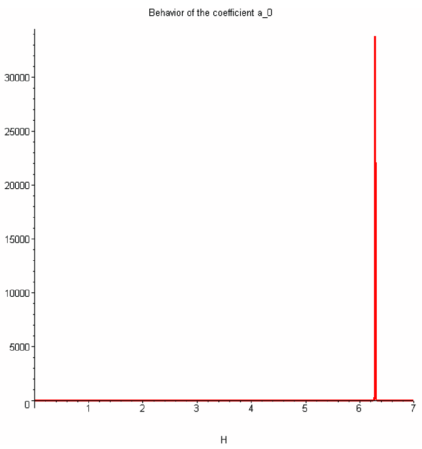
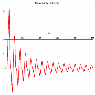
The behavior of the coefficients is given in the following Figure
1.
Figure 1:
Behavior of the coefficient of the new method given by
(LABEL:nm4) for several values of .
The local truncation error of the new proposed method is given by:
(15)
Remark 1
The method developed in this section is the same with the obtained
by Simos in [116]
The application of the above method to the scalar test equation
(LABEL:stab_eq) gives the difference equation (LABEL:nm1) and the
characteristic equation (10).
By applying in the formula (LABEL:phl_multi_defn), we have that
the phase-lag is given by (11). The first derivative of the
phase-lag is given by:
(16)
We demand that the phase-lag and its derivative are equal to zero and we consider that:
(17)
Then we find out that:
(18)
For small values of the formulae given by (18) are
subject to heavy cancelations. In this case the following Taylor
series expansions should be used:
(19)
(20)
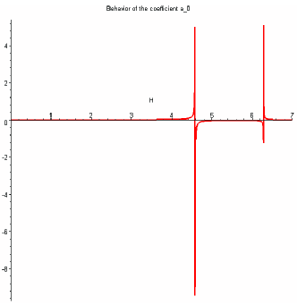
The behavior of the coefficients is given in the following Figure 2.
Figure 2:
Behavior of the coefficients of the new method given by (18)
for several values of .
The local truncation error of the new proposed method is given by:
The application of the above method to the scalar test equation
(LABEL:stab_eq) gives the difference equation (LABEL:nm1) and the
characteristic equation (10).
By applying in the formula (LABEL:phl_multi_defn), we have that
the phase-lag is given by (11). The first derivative of the
phase-lag is given by (16). The second derivative of the
phase-lag can be written as:
(22)
We demand that the phase-lag and its first and second derivative are equal to zero and we consider that:
(23)
Then we find out that:
(24)
For small values of the formulae given by (24) are
subject to heavy cancellations. In this case the following Taylor
series expansions should be used:
(25)
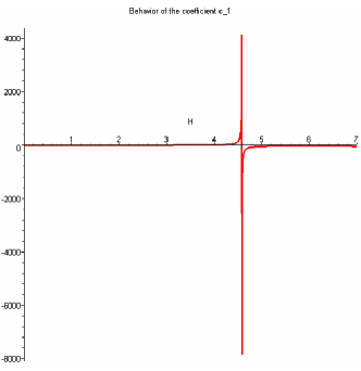
The behavior of the coefficients is given in the following Figure 3.
The local truncation error of the new proposed method is given by:
The application of the above method to the scalar test equation
(LABEL:stab_eq) gives the difference equation (LABEL:nm1) and the
characteristic equation (10).
By applying in the formula (LABEL:phl_multi_defn), we have that
the phase-lag is given by (11). The first derivative of the
phase-lag is given by (16). The second derivative of the
phase-lag is given by (22). The third derivative of the
phase-lag can be written as:
(27)
We demand that the phase-lag and its first, second and third derivative
are equal to zero and we find out that:
(28)
For small values of the formulae given by (28) are
subject to heavy cancellations. In this case the following Taylor
series expansions should be used:
(29)
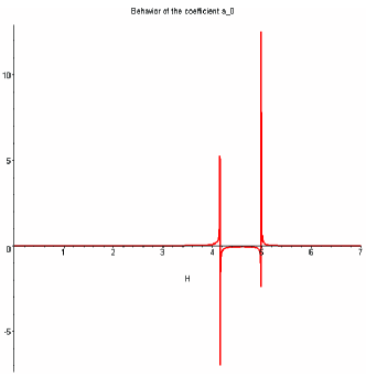
The behavior of the coefficients is given in the following Figure 4.
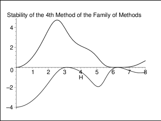
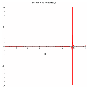
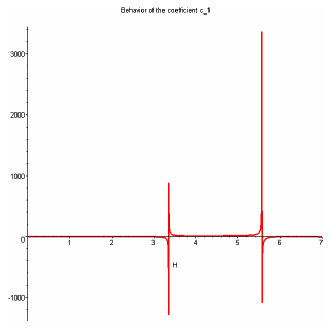
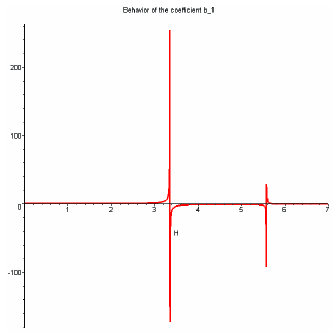
Figure 4:
Behavior of the coefficients of the new method given by (28)
for several values of .
The local truncation error of the new proposed method is given by:
(30)
4 Error Analysis
We will study the following methods:
•
The First Method of the Family (mentioned as )
•
The Second Method of the Family (mentioned as )
•
The Third Method of the Family (mentioned as )
•
The Fourth Method of the
Family (mentioned as )
The error analysis is based on the following steps:
•
The radial time independent Schrödinger equation is of the
form
(31)
•
Based on the paper of Ixaru and Rizea [25], the
function f(x) can be written in the form:
(32)
where , where is the
constant approximation of the potential and .
•
We express the derivatives
which are terms of the local truncation error formulae, in terms
of the equation (LABEL:err1). The expressions are presented as
polynomials of .
•
Finally, we substitute the expressions of the derivatives,
produced in the previous step, into the local truncation error
formulae.
Based on the procedure mentioned above and on the formulae:
we obtain the following expressions:
The First Method of the Family
(33)
The Second Method of the Family
(34)
The Third Method of the Family
(35)
The Fourth Method of the Family
(36)
We consider two cases in terms of the value of :
•
The Energy is close to the potential, i.e. . So only the free terms of the polynomials in are
considered. Thus for these values of , the methods are of
comparable accuracy. This is because the free terms of the
polynomials in , are the same for the cases of the classical
method and of the new developed methods.
•
or . Then is a large number. So,
we have the following asymptotic expansions of the equations
(33), (34), (35) and (36).
The First Method of the Family
(37)
The Second Method of the Family
The Third Method of the Family
(38)
The Fourth Method of the Family
(39)
From the above equations we have the following theorem:
Theorem 2
For the First Method of the New Family of Methods the error
increases as the third power of . For the Second and Third
Methods of the New Family of Methods the error increases as the
second power of . For the Fourth Method of the New Family of
Methods the error increases as the first power of . It is easy
one to see that the coefficient of the second power of in the
case of the second method of the New Family of Methods is
times larger than the coefficient of the second power
of in the case of the third method of the New Family of Methods.
So, for the numerical solution of the time independent radial
Schrödinger equation the new obtained Fourth Method of the New
Family of Methods is the most accurate one, especially for large
values of .
5 Stability Analysis
We apply the new family of methods to the scalar test equation:
(40)
where . We obtain the following difference
equation:
where , is the step length and
and are polynomials of .
The characteristic equation associated with (LABEL:nm1s) is given
by:
(41)
where
(42)
Definition 1
(see [19])
A symmetric four-step method with the characteristic equation given
by (41) is said to have an interval of periodicity
if, for all , the roots satisfy
(43)
where is a real function of and
.
Definition 2
(see [19])
A method is called P-stable if its interval of periodicity is
equal to .
Theorem 3
(see [20])
A symmetric two-step method with the characteristic equation given
by (41) is said to have a nonzero interval of
periodicity if, for all the following relations are hold
(44)
where , and:
(45)
Definition 3
A method is called singularly almost P-stable if its interval of
periodicity is equal to 222where is a set
of distinct points only when the frequency of the phase fitting is
the same as the frequency of the scalar test equation, i.e. .
Based on (42) the stability polynomials (45)
for the new developed methods take the form:
(46)
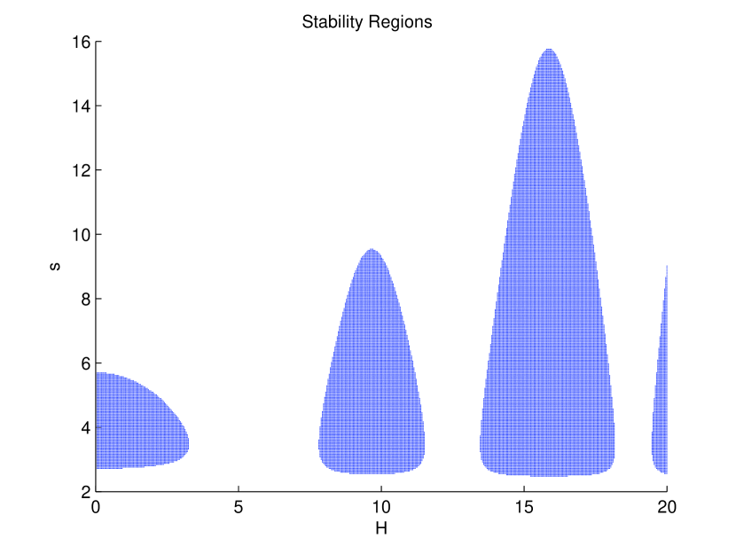
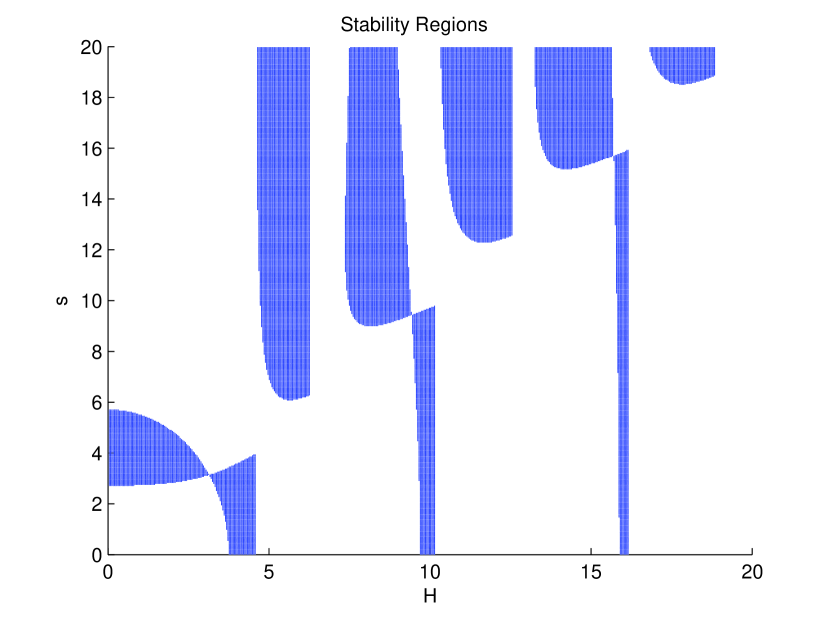
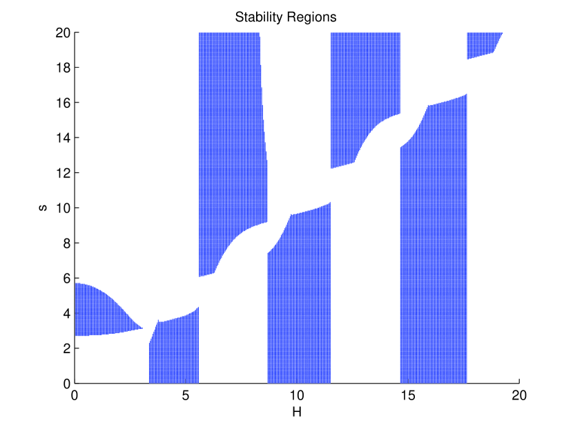
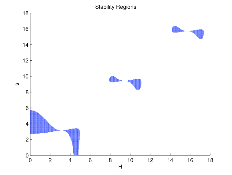
In Figures 5, 6, 7 and 8 we present the planes for the methods developed in this paper. A shadowed area denotes the region where the method is unstable, while a white area denotes the region where the method is stable. In Figure 5 we present the plane for the first method of the new family of method developed in this paper (paragraph 3.1). In Figure 6 we present the plane for the second method of the new family of method developed in this paper (paragraph 3.2). In Figure 7 we present the plane for the third method of the new family of method developed in this paper (paragraph 3.3). Finally, in Figure 8 we present the plane for the fourth method of the new family of method developed in this paper (paragraph 3.4).
Figure 5:
plane of the first method of the new family of method
developed in this paper (paragraph 3.1)Figure 6:
plane of the second method of the new family of method
developed in this paper (paragraph 3.2)Figure 7:
plane of the third method of the new family of method
developed in this paper (paragraph 3.3)Figure 8:
plane of the fourth method of the new family of method
developed in this paper (paragraph 3.4)
Figure 9:
Stability polynomials of the new developed methods in the case that
In the case that the frequency of the scalar test equation is equal
with the frequency of phase fitting, i.e. in the case that , we
have the following figure for the stability polynomials of the new
developed methods. A method is P-stable if the plane is
not shadowed. From the above diagrams it is easy for one to
see that the interval of periodicity of all the new methods is equal
to: .
Remark 2
For the solution of the Schrödinger equation the frequency of
the exponential fitting is equal to the frequency of the scalar
test equation. So, it is necessary to observe the surroundings of
the first diagonal of the plane.
6 Numerical results - Conclusion
In order to illustrate the efficiency of the new methods obtained in
paragraphs 3.1 - 3.4, we apply them to the radial time independent
Schrödinger equation.
In order to apply the new methods to the radial Schrödinger
equation the value of parameter is needed. For every problem of
the one-dimensional Schrödinger equation given by (LABEL:eqn:1)
the parameter is given by
(47)
where is the potential and is the energy.
6.1 Woods-Saxon potential
We use the well known Woods-Saxon potential given by
(48)
with , and
.
The behavior of Woods-Saxon potential is shown in the Figure 10.
Figure 10:
Behavior of the coefficients of the new method given by (24)
for several values of .
It is well known that for some potentials, such as the Woods-Saxon
potential, the definition of parameter is not given as a
function of but it is based on some critical points which have been
defined from the investigation of the appropriate potential (see for
details [13]).
For the purpose of obtaining our numerical results it is
appropriate to choose as follows (see for details
[13]):
(49)
6.2 Radial Schrödinger Equation - The Resonance Problem
Consider the numerical solution of the radial time independent
Schrödinger equation (LABEL:eqn:1) in the well-known case of the
Woods-Saxon potential (LABEL:rkbound2). In order to solve this
problem numerically we need to approximate the true (infinite)
interval of integration by a finite interval. For the purpose of
our numerical illustration we take the domain of integration as . We consider equation (LABEL:eqn:1) in a rather large
domain of energies, i.e. .
In the case of positive energies, , the potential dies
away faster than the term and the
Schrödinger equation effectively reduces to
(50)
for greater than some value .
The above equation has linearly independent solutions
and where and
are the spherical Bessel and Neumann functions respectively. Thus
the solution of equation (LABEL:eqn:1) (when ) has the asymptotic form
(51)
where is the phase shift, that is
calculated from the formula
(52)
for and distinct points in the asymptotic region
(we choose as the right hand end point of the interval of
integration and ) with and
. Since the problem is treated as an
initial-value problem, we need before starting a one-step
method. From the initial condition we obtain . With these
starting values we evaluate at of the asymptotic region
the phase shift .
For positive energies we have the so-called resonance problem.
This problem consists either of finding the phase-shift
or finding those , for , at which
. We actually solve the latter
problem, known as the resonance problem when the positive
eigenenergies lie under the potential barrier.
The boundary conditions for this problem are:
(53)
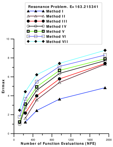
Figure 11:
Error Errmax for several values of n for the eigenvalue . The nonexistence of a value of Errmax indicates that
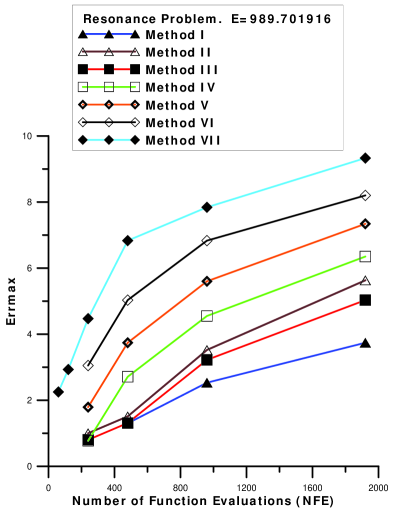
for this value of n, Errmax is positiveFigure 12:
Error Errmax for several values of n for the eigenvalue . The nonexistence of a value of Errmax indicates that
for this value of n, Errmax is positive
We compute the approximate positive eigenenergies of the
Woods-Saxon resonance problem using:
•
The Numerov’s method which is indicated as Method I
•
The Exponentially-fitted four-step method developed by Raptis [16] which is indicated as
Method II
•
The Two-Step Numerov-type Method with minimum phase-lag produced by Chawla and Rao [23] which is indicated as Method III
•
The new Two-Step Numerov-Type Method with phase-lag equal to zero obtained in paragraph 3.1 which is indicated as Method IV.
•
The new Two-Step Numerov-Type Method with phase-lag and its first derivative equal to zero obtained in paragraph 3.2 which is indicated as Method V.
•
The new Two-Step Numerov-Type Method with phase-lag and its first and second derivatives equal to zero obtained in paragraph 3.3 which is indicated as Method VI.
•
The new Two-Step Numerov-Type Method with phase-lag and its first, second and third derivatives equal to zero obtained in paragraph 3.4 which is indicated as Method VII.
The computed eigenenergies are compared with exact ones. In Figure
11 we present the maximum absolute error where
(54)
of the eigenenergy , for several values of
NFE = Number of Function Evaluations. In Figure 12 we present the maximum absolute error
where
(55)
of the eigenenergy , for several values of
NFE = Number of Function Evaluations.
7 Conclusions
In the present paper we have developed a family of methods of sixth
algebraic order for the numerical solution of the radial
Schrödinger equation.
More specifically we have developed:
1.
A Two-Step Numerov-Type Method with phase-lag equal to zero
2.
A Two-Step Numerov-Type Method with phase-lag and its first derivative equal to zero
3.
A Two-Step Numerov-Type Method with phase-lag and its first and second derivatives equal to zero
4.
A Two-Step Numerov-Type Method with phase-lag and its first, second and third derivatives equal to zero
We have applied the new method to the resonance problem of the
radial Schrödinger equation.
Based on the results presented above we have the following
conclusions:
•
The Exponentially-fitted four-step method developed by Raptis [16] (denoted as Method II) is more efficient than the Numerov’s Method (denoted Method I).
•
The Two-Step Numerov-type Method with minimum phase-lag produced by Chawla and Rao [23] (Method III) is more efficient than the Exponentially-fitted four-step method developed by Raptis [16] (Method II) for the energy
and less efficient for the energy .
•
The new developed methods are much more efficient than the older ones.
•
The Two-Step Numerov-Type Method with phase-lag and its first derivative equal to zero (Method V) is more efficient than the New Two-Step Numerov-Type Method with phase-lag equal to zero
(Method IV)
•
The Two-Step Numerov-Type Method with phase-lag and its first and second derivatives equal to zero (Method VI) is more efficient than the Two-Step Numerov-Type Method with phase-lag and its first derivative equal to zero (Method V)
•
The Two-Step Numerov-Type Method with phase-lag and its first, second and third derivatives equal to zero (Method VII) is more efficient than the Two-Step Numerov-Type Method with phase-lag and its first and second derivatives equal to zero (Method VI)
All computations were carried out on a IBM PC-AT compatible 80486
using double precision arithmetic with 16 significant digits
accuracy (IEEE standard).
References
[1] L.Gr. Ixaru and M. Micu,
Topics in Theoretical Physics. Central Institute of Physics,
Bucharest, 1978.
[2] L.D. Landau and F.M.
Lifshitz: Quantum Mechanics. Pergamon, New York, 1965.
[3] I. Prigogine,
Stuart Rice (Eds): Advances in Chemical Physics Vol. 93: New
Methods in Computational Quantum Mechanics, John Wiley & Sons,
1997.
[4] G. Herzberg, Spectra of
Diatomic Molecules, Van Nostrand, Toronto, 1950.
[5] T.E. Simos, Atomic Structure
Computations in Chemical Modelling: Applications and Theory
(Editor: A. Hinchliffe, UMIST), The Royal Society of
Chemistry 38-142(2000).
[6] T.E. Simos, Numerical
methods for 1D, 2D and 3D differential equations arising in
chemical problems, Chemical Modelling: Application and
Theory, The Royal Society of Chemistry, 2(2002),170-270.
[7] T.E. Simos and
P.S. Williams, On finite difference methods for the solution of
the Schrödinger equation, Computers & Chemistry23
513-554(1999).
[8] T.E. Simos: Numerical
Solution of Ordinary Differential Equations with Periodical
Solution. Doctoral Dissertation, National Technical University of
Athens, Greece, 1990 (in Greek).
[9] A. Konguetsof and T.E.
Simos, On the Construction of exponentially-fitted methods for the
numerical solution of the Schrödinger Equation, Journal of
Computational Methods in Sciences and Engineering1
143-165(2001).
[10] A.D. Raptis and A.C.
Allison: Exponential - fitting methods for the numerical
solution of the Schrödinger equation, Computer Physics
Communications, 14 1-5(1978).
[11] A.D. Raptis, Exponential
multistep methods for ordinary differential equations, Bull.
Greek Math. Soc.25 113-126(1984).
[12] L.Gr. Ixaru, Numerical Methods
for Differential Equations and Applications, Reidel, Dordrecht -
Boston - Lancaster, 1984.
[13] L.Gr. Ixaru and M. Rizea,
A Numerov-like scheme for the numerical solution of the
Schrödinger equation in the deep continuum spectrum of
energies. Comput. Phys. Commun. 19 23-27(1980).
[14] T. E. Simos, P. S.
Williams: A New Runge-Kutta-Nystrom Method with Phase-Lag of Order
Infinity for the Numerical Solution of the Schrödinger Equation,
MATCH Commun. Math. Comput. Chem.45 123-137(2002).
[15] T. E. Simos, Multiderivative
Methods for the Numerical Solution of the Schrödinger Equation,
MATCH Commun. Math. Comput. Chem.45 7-26(2004).
[16] A.D. Raptis, Exponentially-fitted solutions of the
eigenvalue Shrödinger equation with automatic error control,
Computer Physics Communications, 28 427-431(1983)
[17] A.D. Raptis, On the numerical solution of the Schrodinger
equation, Computer Physics Communications, 24
1-4(1981)
[18] Zacharoula Kalogiratou and T.E. Simos, A P-stable exponentially-fitted method for the numerical
integration of the Schrödinger equation, Applied
Mathematics and Computation, 112 99-112(2000).
[19] J.D. Lambert and I.A.
Watson, Symmetric multistep methods for periodic initial values
problems, J. Inst. Math. Appl.18 189-202(1976).
[20] A.D. Raptis and T.E. Simos, A four-step phase-fitted method for the numerical integration
of second order initial-value problem, BIT, 31
160-168(1991).
[21] Peter Henrici, Discrete variable methods in ordinary differential equations, John Wiley
& Sons, 1962.
[22] M.M. Chawla, Uncoditionally stable Noumerov-type methods for second order differential equations, BIT,
23 541-542(1983).
[23] M. M. Chawla and P. S. Rao, A Noumerov-type method with minimal phase-lag for the integration of second order periodic initial-value problems, Journal of Computational and Applied Mathematics11(3)
277-281(1984)
[24] Liviu Gr. Ixaru and Guido Vanden Berghe,
Exponential Fitting, Series on Mathematics and its Applications,
Vol. 568, Kluwer Academic Publisher, The Netherlands, 2004.
[25] L. Gr. Ixaru and M. Rizea, Comparison of some four-step methods for the numerical solution of the Schrödinger equation, Computer
Physics Communications, 38(3) 329-337(1985)
[26]
Z.A. Anastassi, T.E. Simos, A family of exponentially-fitted Runge-Kutta methods with exponential order up to three for the numerical solution of the Schrödinger equation, J. Math. Chem41 (1) 79-100 (2007)
[27]
T. Monovasilis, Z. Kalogiratou , T.E. Simos, Trigonometrically
fitted and exponentially fitted symplectic methods for the
numerical integration of the
Schrödinger equation, J. Math. Chem40 (3) 257-267
(2006)
[28]
G. Psihoyios, T.E. Simos, The numerical solution of the radial
Schrödinger equation via a trigonometrically fitted family of
seventh algebraic order
Predictor-Corrector methods, J. Math. Chem40 (3)
269-293 (2006)
[29]
T.E. Simos, A four-step exponentially fitted method for the
numerical solution of the Schrödinger equation, J. Math.
Chem40 (3) 305-318
(2006)
[30]
T. Monovasilis, Z. Kalogiratou , T.E. Simos, Exponentially fitted
symplectic methods for the numerical integration of the
Schrödinger equation J. Math. Chem37 (3) 263-270
(2005)
[31]
Z. Kalogiratou , T. Monovasilis, T.E. Simos, Numerical solution of
the two-dimensional time independent Schrödinger equation with
Numerov-type methods J. Math. Chem37 (3) 271-279
(2005)
[32]
Z.A. Anastassi, T.E. Simos, Trigonometrically fitted Runge-Kutta
methods for the numerical solution of the Schrödinger equation
J. Math. Chem37 (3) 281-293 (2005)
[33]
G. Psihoyios, T.E. Simos, Sixth algebraic order trigonometrically
fitted predictor-corrector methods for the numerical solution of
the radial Schrödinger
equation, J. Math. Chem37 (3) 295-316 (2005)
[34]
D.P. Sakas, T.E. Simos, A family of multiderivative methods for
the numerical solution of the Schrödinger equation, J.
Math. Chem37 (3)
317-331 (2005)
[35]
T.E. Simos, Exponentially - fitted multiderivative methods for the
numerical solution of the Schrödinger equation, J. Math.
Chem36 (1) 13-27 (2004)
[36]
K. Tselios, T.E. Simos, Symplectic methods of fifth order for the
numerical solution of the radial Shrodinger equation, J.
Math. Chem35 (1)
55-63 (2004)
[37]
T.E. Simos, A family of trigonometrically-fitted symmetric methods
for the efficient solution of the Schrödinger equation and
related problems J. Math. Chem34 (1-2) 39-58 JUL 2003
[38]
K. Tselios, T.E. Simos, Symplectic methods for the numerical
solution of the radial Shrödinger equation, J. Math. Chem34 (1-2) 83-94 (2003)
[39]
J. Vigo-Aguiar J, T.E. Simos, Family of twelve steps exponential
fitting symmetric multistep methods for the numerical solution of
the Schrödinger equation, J. Math. Chem32 (3)
257-270 (2002)
[40]
G. Avdelas, E. Kefalidis, T.E. Simos, New P-stable eighth
algebraic order exponentially-fitted methods for the numerical
integration of the Schrödinger equation, J. Math. Chem31 (4) 371-404 (2002)
[41]
T.E. Simos, J. Vigo-Aguiar, Symmetric eighth algebraic order
methods with minimal phase-lag for the numerical solution of the
Schrödinger equation J. Math. Chem31 (2) 135-144
(2002)
[42]
Z. Kalogiratou , T.E. Simos, Construction of trigonometrically and
exponentially fitted Runge-Kutta-Nystrom methods for the numerical
solution of the Schrödinger equation and related problems a
method of 8th algebraic order, J. Math. Chem31 (2)
211-232
[43]
T.E. Simos, J. Vigo-Aguiar, A modified phase-fitted Runge-Kutta
method for the numerical solution of the Schrödinger equation,
J. Math. Chem30 (1) 121-131 (2001)
[44]
G. Avdelas, A. Konguetsof, T.E. Simos, A generator and an
optimized generator of high-order hybrid explicit methods for the
numerical solution of the Schrödinger equation. Part 1.
Development of the basic method, J. Math. Chem29 (4)
281-291 (2001)
[45]
G. Avdelas, A. Konguetsof, T.E. Simos, A generator and an
optimized generator of high-order hybrid explicit methods for the
numerical solution of the Schrödinger equation. Part 2.
Development of the generator; optimization of the generator and
numerical results, J. Math. Chem29 (4) 293-305 (2001)
[46]
J. Vigo-Aguiar, T.E. Simos, A family of P-stable eighth algebraic
order methods with exponential fitting facilities, J. Math.
Chem29 (3) 177-189 (2001)
[47]
T.E. Simos, A new explicit Bessel and Neumann fitted eighth
algebraic order method for the numerical solution of the
Schrödinger equation J. Math. Chem27 (4) 343-356
(2000)
[48]
G. Avdelas, T.E. Simos, Embedded eighth order methods for the
numerical solution of the Schrödinger equation, J. Math.
Chem26 (4) 327-341 1999,
[49]
T.E. Simos, A family of P-stable exponentially-fitted methods for
the numerical solution of the Schrödinger equation, J.
Math. Chem25 (1) 65-84 (1999)
[50]
T.E. Simos, Some embedded modified Runge-Kutta methods for the
numerical solution of some specific Schrödinger equations, J. Math. Chem24 (1-3) 23-37 (1998)
[51]
T.E. Simos, Eighth order methods with minimal phase-lag for
accurate computations for the elastic scattering phase-shift
problem, J. Math. Chem21 (4) 359-372 (1997)
[52]
P. Amodio, I. Gladwell and G. Romanazzi, Numerical Solution of
General Bordered ABD Linear Systems by Cyclic Reduction, JNAIAM J. Numer. Anal. Indust. Appl. Math1(1) 5-12(2006)
[53]
S. D. Capper, J. R. Cash and D. R. Moore, Lobatto-Obrechkoff
Formulae for 2nd Order Two-Point Boundary Value Problems, JNAIAM J. Numer. Anal. Indust. Appl. Math1(1) 13-25 (2006)
[54]
S. D. Capper and D. R. Moore, On High Order MIRK Schemes and
Hermite-Birkhoff Interpolants, JNAIAM J. Numer. Anal. Indust.
Appl. Math1(1) 27-47 (2006)
[55]
J. R. Cash, N. Sumarti, T. J. Abdulla and I. Vieira, The
Derivation of Interpolants for Nonlinear Two-Point Boundary Value
Problems, JNAIAM J. Numer. Anal. Indust. Appl. Math1(1) 49-58 (2006)
[56]
J. R. Cash and S. Girdlestone, Variable Step Runge-Kutta-Nystr m
Methods for the Numerical Solution of Reversible Systems, JNAIAM J. Numer. Anal. Indust. Appl. Math1(1) 59-80 (2006)
[57]
Jeff R. Cash and Francesca Mazzia, Hybrid Mesh Selection
Algorithms Based on Conditioning for Two-Point Boundary Value
Problems, JNAIAM J. Numer. Anal. Indust. Appl. Math1(1) 81-90 (2006)
[58]
Felice Iavernaro, Francesca Mazzia and Donato Trigiante, Stability
and Conditioning in Numerical Analysis, JNAIAM J. Numer.
Anal. Indust. Appl. Math1(1) 91-112 (2006)
[59]
Felice Iavernaro and Donato Trigiante, Discrete Conservative
Vector Fields Induced by the Trapezoidal Method, JNAIAM J.
Numer. Anal. Indust. Appl. Math1(1) 113-130 (2006)
[60]
Francesca Mazzia, Alessandra Sestini and Donato Trigiante, BS
Linear Multistep Methods on Non-uniform Meshes, JNAIAM J.
Numer. Anal. Indust. Appl. Math1(1) 131-144 (2006)
[61]
L.F. Shampine, P.H. Muir, H. Xu, A User-Friendly Fortran BVP
Solver, JNAIAM J. Numer. Anal. Indust. Appl. Math1(2)
201-217 (2006)
[62]
G. Vanden Berghe and M. Van Daele, Exponentially- fitted
St rmer/Verlet methods, JNAIAM J. Numer. Anal. Indust. Appl.
Math1(3) 241-255 (2006)
[63]
L. Aceto, R. Pandolfi, D. Trigiante, Stability Analysis of Linear
Multistep Methods via Polynomial Type Variation, JNAIAM J.
Numer. Anal. Indust. Appl. Math2(1-2) 1-9 (2007)
[64] G. Psihoyios, A Block Implicit Advanced Step-point (BIAS) Algorithm for Stiff Differential
Systems, Computing Letters2(1-2) 51-58(2006)
[65] W.H. Enright, On the use of ’arc length’ and ’defect’
for mesh selection for differential equations, Computing
Letters1(2) 47-52(2005)
[66]
T.E. Simos, P-stable Four-Step Exponentially-Fitted Method for the
Numerical Integration of the Schrödinger Equation, Computing Letter1(1) 37-45(2005).
[67]
T.E. Simos, Stabilization of a Four-Step Exponentially-Fitted
Method and its Application to the Schrödinger Equation, International Journal of Modern Physics C18(3)
315-328(2007).
[68]
Zhongcheng Wang, P-stable linear symmetric multistep methods for
periodic initial-value problems, Computer Physics
Communications171 162 174(2005)
[69] T.E. Simos, A Runge-Kutta Fehlberg method with phase-lag of order
infinity for initial value problems with oscillating solution, Computers and Mathematics with Applications25 95-101(1993).
[70] T.E. Simos, Runge-Kutta interpolants with minimal phase-lag,
Computers and Mathematics with Applications26
43-49(1993).
[71] T.E. Simos, Runge-Kutta-Nyström interpolants for the numerical
integration of special second-order periodic initial-value problems,
Computers and Mathematics with Applications26
7-15(1993).
[72] T.E. Simos and G.V. Mitsou, A family of four-step exponential fitted
methods for the numerical integration of the radial Schrödinger
equation, Computers and Mathematics with Applications28
41-50(1994).
[73] T.E. Simos and G. Mousadis, A two-step method for the numerical
solution of the radial Schr dinger equation, Computers and
Mathematics with Applications29 31-37(1995).
[74] G. Avdelas and T.E. Simos, Block Runge-Kutta methods for periodic
initial-value problems, Computers and Mathematics with
Applications31 69- 83(1996).
[75] G. Avdelas and T.E. Simos, Embedded methods for the numerical
solution of the Schrödinger equation, Computers and
Mathematics with Applications31 85-102(1996).
[76] G. Papakaliatakis and T.E. Simos, A new method for the numerical
solution of fourth order BVP s with oscillating solutions, Computers and Mathematics with Applications32 1-6(1996).
[77] T.E. Simos, An extended Numerov-type method for the numerical
solution of the Schrödinger equation, Computers and
Mathematics with Applications33 67-78(1997).
[78] T.E. Simos, A new hybrid imbedded variable-step procedure for the
numerical integration of the Schrödinger equation, Computers
and Mathematics with Applications36 51-63(1998).
[79] T.E. Simos, Bessel and Neumann Fitted Methods for the Numerical
Solution of the Schrödinger equation, Computers &
Mathematics with Applications42 833-847(2001).
[80] A. Konguetsof and T.E. Simos, An exponentially-fitted and
trigonometrically-fitted method for the numerical solution of
periodic initial-value problems, Computers and Mathematics with
Applications45 547-554(2003).
[81] Z.A. Anastassi and T.E. Simos, An optimized Runge-Kutta method for the solution of orbital problems, Journal of Computational and Applied Mathematics175(1) 1-9(2005)
[82] G. Psihoyios and T.E. Simos, A fourth algebraic order trigonometrically fitted predictor-corrector scheme for IVPs with
oscillating solutions, Journal of Computational and Applied
Mathematics175(1) 137-147(2005)
[83] D.P. Sakas and T.E. Simos, Multiderivative methods of eighth algrebraic order with minimal phase-lag for the numerical solution of
the radial Schrödinger equation, Journal of Computational and
Applied Mathematics 175(1) 161-172(2005)
[84] K. Tselios and T.E. Simos, Runge-Kutta methods with minimal dispersion and dissipation for problems arising from computational acoustics, Journal of Computational and Applied Mathematics175(1) 173-181(2005)
[85] Z. Kalogiratou and T.E. Simos, Newton-Cotes formulae for long-time integration, Journal of Computational and Applied Mathematics158(1) 75-82(2003)
[86] Z. Kalogiratou, T. Monovasilis and T.E. Simos, Symplectic integrators for the numerical solution of the Schrödinger equation, Journal of Computational and Applied Mathematics158(1) 83-92(2003)
[87] A. Konguetsof and T.E. Simos, A generator of hybrid symmetric four-step methods for the numerical solution of the Schrödinger equation, Journal of Computational and Applied Mathematics158(1) 93-106(2003)
[88] G. Psihoyios and T.E. Simos, Trigonometrically fitted predictor-corrector methods for IVPs with oscillating solutions, Journal of Computational and Applied Mathematics158(1) 135-144(2003)
[89] Ch. Tsitouras and T.E. Simos, Optimized Runge-Kutta pairs for problems with oscillating solutions, Journal of Computational and Applied Mathematics147(2) 397-409(2002)
[90] T.E. Simos, An exponentially fitted eighth-order method for the numerical solution of the Schrödinger equation, Journal of Computational and Applied Mathematics108(1-2)
177-194(1999)
[91] T.E. Simos, An accurate finite difference method for the numerical solution of the Schrödinger equation, Journal of Computational and Applied Mathematics91(1) 47-61(1998)
[92] R.M. Thomas and T.E. Simos, A family of hybrid exponentially fitted predictor-corrector methods for the
numerical integration of the radial Schrödinger equation, Journal of Computational and Applied Mathematics87(2)
215-226(1997)
[93] Z.A. Anastassi and T.E. Simos: Special Optimized Runge-Kutta methods for IVPs with Oscillating Solutions, International Journal of Modern Physics C, 15, 1-15 (2004)
[94] Z.A. Anastassi and T.E. Simos: A Dispersive-Fitted and Dissipative-Fitted Explicit Runge-Kutta method for the Numerical Solution of Orbital Problems, New Astronomy, 10, 31-37 (2004)
[95] Z.A. Anastassi and T.E. Simos: A Trigonometrically-Fitted Runge-Kutta Method for the Numerical Solution of Orbital Problems, New Astronomy, 10, 301-309 (2005)
[96] T.V. Triantafyllidis, Z.A. Anastassi and T.E. Simos: Two Optimized Runge-Kutta Methods for the Solution of the Schr?dinger Equation, MATCH Commun. Math. Comput. Chem., 60, 3 (2008)
[97] Z.A. Anastassi and T.E. Simos, Trigonometrically Fitted Fifth Order Runge-Kutta Methods for the Numerical Solution of the Schrödinger Equation, Mathematical and Computer Modelling, 42 (7-8), 877-886 (2005)
[98] Z.A. Anastassi and T.E. Simos: New Trigonometrically Fitted Six-Step Symmetric Methods for the Efficient Solution of the Schrödinger Equation, MATCH Commun. Math. Comput. Chem., 60, 3 (2008)
[99] G.A. Panopoulos, Z.A. Anastassi and T.E. Simos: Two New Optimized Eight-Step Symmetric Methods for the Efficient Solution of the Schrödinger Equation and Related Problems, MATCH Commun. Math. Comput. Chem., 60, 3 (2008)
[100] Z.A. Anastassi and T.E. Simos: A Six-Step P-stable Trigonometrically-Fitted Method for the Numerical Integration of the Radial Schrödinger Equation, MATCH Commun. Math. Comput. Chem., 60, 3 (2008)
[101] Z.A. Anastassi and T.E. Simos, A family of two-stage two-step methods for the numerical integration of the Schrödinger equation and related IVPs with oscillating solution, Journal of Mathematical Chemistry, Article in Press, Corrected Proof
[102] T.E. Simos and P.S. Williams, A finite-difference method for the numerical solution of the Schrödinger equation, Journal of Computational and Applied Mathematics79(2) 189-205(1997)
[103] G. Avdelas and T.E. Simos, A generator of high-order embedded P-stable methods for the numerical solution of the
Schrödinger equation, Journal of Computational and Applied
Mathematics72(2) 345-358(1996)
[104] R.M. Thomas, T.E. Simos and G.V. Mitsou, A family of Numerov-type exponentially fitted predictor-corrector methods for the
numerical integration of the radial Schrödinger equation, Journal of Computational and Applied Mathematics67(2)
255-270(1996)
[105] T.E. Simos, A Family of 4-Step Exponentially Fitted Predictor-Corrector Methods for the Numerical-Integration of
The Schrödinger-Equation, Journal of Computational and
Applied Mathematics58(3) 337-344(1995)
[106] T.E. Simos, An Explicit 4-Step Phase-Fitted Method for the Numerical-Integration of 2nd-order Initial-Value Problems, Journal of Computational and Applied Mathematics55(2) 125-133(1994)
[107] T.E. Simos, E. Dimas and A.B. Sideridis, A Runge-Kutta-Nyström Method for the Numerical-Integration of Special 2nd-order
Periodic Initial-Value Problems, Journal of Computational and
Applied Mathematics51(3) 317-326(1994)
[108] A.B. Sideridis and T.E. Simos, A Low-Order Embedded Runge-Kutta Method for Periodic Initial-Value Problems, Journal of Computational and Applied Mathematics44(2) 235-244(1992)
[109] T.E. Simos amd A.D. Raptis, A 4th-order Bessel Fitting Method for the Numerical-Solution of the SchrÖdinger-Equation, Journal of Computational and Applied Mathematics43(3)
313-322(1992)
[110] T.E. Simos, Explicit 2-Step Methods with Minimal Phase-Lag for the Numerical-Integration of Special 2nd-order Initial-Value
Problems and their Application to the One-Dimensional
Schrödinger-Equation, Journal of Computational and Applied
Mathematics39(1) 89-94(1992)
[111] T.E. Simos, A 4-Step Method for the Numerical-Solution of the Schrödinger-Equation, Journal of Computational and Applied Mathematics30(3) 251-255(1990)
[112] C.D. Papageorgiou, A.D. Raptis and T.E. Simos, A Method for Computing Phase-Shifts for Scattering, Journal of Computational and Applied
Mathematics29(1) 61-67(1990)
[113] A.D. Raptis, Two-Step Methods for the Numerical Solution of the Schrödinger Equation, Computing28 373-378(1982).
[114] T.E. Simos. A new Numerov-type method for computing eigenvalues and resonances of the radial Schrödinger
equation, International Journal of Modern Physics C-Physics and
Computers, 7(1) 33-41(1996)
[115] T.E. Simos, Predictor Corrector Phase-Fitted Methods for Y”=F(X,Y) and an Application to the
Schrödinger-Equation, International Journal of Quantum Chemistry,
53(5) 473-483(1995)
[116] T.E. Simos, Two-step almost P-stable complete
in phase methods for the numerical integration of second order
periodic initial-value problems, Inter. J. Comput. Math.46 77-85(1992).
[117] R. M. Corless, A. Shakoori, D.A. Aruliah, L. Gonzalez-Vega, Barycentric Hermite Interpolants for Event Location in Initial-Value Problems, JNAIAM J. Numer. Anal. Indust. Appl. Math, 3, 1-16 (2008)
[118] M. Dewar, Embedding a General-Purpose Numerical Library in an Interactive Environment, JNAIAM J. Numer. Anal. Indust. Appl. Math, 3, 17-26 (2008)
[119] J. Kierzenka and L.F. Shampine, A BVP Solver that Controls Residual and Error, JNAIAM J. Numer. Anal. Indust. Appl. Math, 3, 27-41 (2008)
[120] R. Knapp, A Method of Lines Framework in Mathematica, JNAIAM J. Numer. Anal. Indust. Appl. Math, 3, 43-59 (2008)
[121] N. S. Nedialkov and J. D. Pryce, Solving Differential Algebraic Equations by Taylor Series (III): the DAETS Code, JNAIAM J. Numer. Anal. Indust. Appl. Math, 3, 61-80 (2008)
[122] R. L. Lipsman, J. E. Osborn, and J. M. Rosenberg, The SCHOL Project at the University of Maryland: Using Mathematical Software in the Teaching of Sophomore Differential Equations, JNAIAM J. Numer. Anal. Indust. Appl. Math, 3, 81-103 (2008)
[123] M. Sofroniou and G. Spaletta, Extrapolation Methods in Mathematica, JNAIAM J. Numer. Anal. Indust. Appl. Math, 3, 105-121 (2008)
[124] R. J. Spiteri and Thian-Peng Ter, pythNon: A PSE for the Numerical Solution of Nonlinear Algebraic Equations, JNAIAM J. Numer. Anal. Indust. Appl. Math, 3, 123-137 (2008)
[125] S.P. Corwin, S. Thompson and S.M. White, Solving ODEs and DDEs with Impulses, JNAIAM J. Numer. Anal. Indust. Appl. Math, 3, 139-149 (2008)
[126] W. Weckesser, VFGEN: A Code Generation Tool, JNAIAM J. Numer. Anal. Indust. Appl. Math, 3, 151-165 (2008)
[127] A. Wittkopf, Automatic Code Generation and Optimization in Maple, JNAIAM J. Numer. Anal. Indust. Appl. Math, 3, 167-180 (2008)