Two Optimized Symmetric Eight-Step Implicit Methods for Initial-Value Problems with Oscillating Solutions

Abstract

In this paper we present two optimized eight-step symmetric implicit methods with phase-lag order ten and infinite (phase-fitted). The methods are constructed to solve numerically the radial time-independent Schrödinger equation with the use of the Woods-Saxon potential. They can also be used to integrate related IVPs with oscillating solutions such as orbital problems. We compare the two new methods to some recently constructed optimized methods from the literature. We measure the efficiency of the methods and conclude that the new method with infinite order of phase-lag is the most efficient of all the compared methods and for all the problems solved.

0.260, 95.10.E

1 Introduction

The radial Schrödinger equation can be written as:

$$y^{\prime\prime}(r)=\left(\frac{l(l+1)}{r^{2}}+V(r)-E\right)y(r)$$ (1)

where $\frac{l(l+1)}{r^{2}}$ is the centrifugal potential, $V(r)$ is the potential, $E$ is the energy and $W(r)=\frac{l(l+1)}{r^{2}}+V(r)$ is the effective potential. It is valid that ${\mathop{\lim}\limits_{r\to\infty}}V(r)=0$ and therefore ${\mathop{\lim}\limits_{r\to\infty}}W(r)=0$.

We consider $E>0$ and divide $[0,\infty)$ into subintervals $[a_{i},b_{i}]$ so that $W(r)$ is a constant with value ${\mathop{W_{i}}\limits^{\_}}$. After this the problem (1) can be expressed by the approximation:

$$\begin{array}[]{l}y^{\prime\prime}_{i}=({\mathop{W}\limits^{\_}}-E)\,y_{i},\\ \end{array}$$ (2)

whose solution is:

$$\begin{array}[]{l}y_{i}(r)=A_{i}\,\exp{\left(\sqrt{{\mathop{W}\limits^{\_}}-E}\,r\right)}+B_{i}\,\exp{\left(-\sqrt{{\mathop{W}\limits^{\_}}-E}\,r\right)},\\ A_{i},\,B_{i}\,\in{\mathbb{R}}.\end{array}$$ (3)

Many numerical methods have been developed for the efficient solution of the Schrödinger equation and related problems. For example Raptis and Allison have developed a two-step exponentially-fitted method of order four in [5]. More recently Kalogiratou and Simos have constructed a two-step P-stable exponentially-fitted method of order four in [6].

Some other notable multistep methods for the numerical solution of oscillating IVPs have been developed by Chawla and Rao in [3], who produced a three-stage, two-Step P-stable method with minimal phase-lag and order six and by Henrici in [4], who produced a four-step symmetric method of order six. Also Anastassi and Simos have developed trigonometrically fitted six-step symmetric methods in [108] and a six-step P-stable trigonometrically-fitted method in [110] and Panopoulos, Anastassi and Simos have constructed two optimized eight-step symmetric methods.

Also some research work in numerical methods can be found in [1]-[137].

2 Phase-lag analysis of symmetric multistep methods

For the numerical solution of the initial value problem

$$y^{\prime\prime}=f(x,y)$$ (4)

multistep methods of the form

$$\sum\limits_{i=0}^{m}{a_{i}y_{n+i}}=h^{2}\sum\limits_{i=0}^{m}{b_{i}f(x_{n+i},y_{n+i})}$$ (5)

with $m$ steps can be used over the equally spaced intervals $\left\{x_{i}\right\}^{m}_{i=0}\in[a,b]$ and $h=|x_{i+1}-x_{i}|$,   $i=0(1)m-1$.

If the method is symmetric then $a_{i}=a_{m-i}$ and $b_{i}=b_{m-i}$,   $i=0(1)\lfloor\frac{m}{2}\rfloor$.

Method (5) is associated with the operator

$$L(x)=\sum\limits_{i=0}^{m}{a_{i}u(x+ih)}-h^{2}\sum\limits_{i=0}^{m}{b_{i}u^{\prime\prime}(x+ih)}$$ (6)

where $u\in C^{2}$.

Definition 1

The multistep method (5) is called algebraic of order $p$ if the associated linear operator $L$ vanishes for any linear combination of the linearly independent functions $\,1,\,x,\,x^{2},\,\ldots,\,x^{p+1}$.

When a symmetric $2k$-step method, that is for $i=-k(1)k$, is applied to the scalar test equation

$$y^{\prime\prime}=-\omega^{2}y$$ (7)

a difference equation of the form

$$A_{k}(v)y_{n+k}+...+A_{1}(v)y_{n+1}+A_{0}(v)y_{n}$$

$$+A_{1}(v)y_{n-1}+...+A_{k}(v)y_{n-k}=0$$ (8)

is obtained, where $v=\omega h$, $h$ is the step length and $A_{0}(v)$, $A_{1}(v),\ldots$, $A_{k}(v)$ are polynomials of $v$.

The characteristic equation associated with (2) is

$$A_{k}(v)s^{k}+...+A_{1}(v)s+A_{0}(v)+A_{1}(v)s^{-1}+...+A_{k}(v)s^{-k}=0$$ (9)

From Lambert and Watson (1976) we have the following definitions:

Definition 2

A symmetric $2k$-step method with characteristic equation given by (9) is said to have an interval of periodicity $(0,v_{0}^{2})$ if, for all $v\in(0,v_{0}^{2}),$ the roots $s_{i},i=1(1)2k$ of Eq. (9) satisfy:

$$s_{1}=e^{i\theta(v)},\,s_{2}=e^{-i\theta(v)},\,\,and\,\,|s_{i}|\leq 1,\,i=3(1)2k$$ (10)

where $\theta(v)$ is a real function of v.

Definition 3

For any method corresponding to the characteristic equation (9) the phase-lag is defined as the leading term in the expansion of

$$t=v-\theta(v)$$ (11)

Then if the quantity $t=O(v^{q+1})\,\,as\,\,{v\to\infty},$ the order phase-lag is q.

Theorem 1

[1] The symmetric $2k$-step method with characteristic equation given by (9) has phase-lag order $q$ and phase-lag constant $c$ given by

$$-cv^{q+2}+O(v^{q+4})={\frac{{2A_{k}(v)\cos(kv)+...+2A_{j}(v)\cos(jv)+...+A_{0}(v)}}{{2k^{2}A_{k}(v)+...+2j^{2}A_{j}(v)+...+2A_{1}(v)}}}$$ (12)

The formula proposed from the above theorem gives us a direct method to calculate the phase-lag of any symmetric $2k$- step method.

In our case, the symmetric 8-step method has phase-lag order $q$ and phase-lag constant $c$ given by:

$$\begin{array}[]{l}{-cv^{q+2}+O(v^{q+4})=}\\ {\frac{{2A_{4}(v)\cos(4v)+2A_{3}(v)\cos(3v)+2A_{2}(v)\cos(2v)+2A_{1}(v)\cos(v)+A_{0}(v)}}{{32A_{4}(v)+18A_{3}(v)+8A_{2}(v)+2A_{1}(v)}}}\end{array}$$ (13)

3 Construction of the new optimized multistep methods

We consider the eight-step symmetric implicit methods of the form:

$$\begin{array}[]{c}y_{{4}}=-y_{{-4}}-a_{{3}}(y_{{3}}+y_{{-3}})-a_{{2}}(y_{{2}}+y_{{-2}})-a_{{1}}(y_{{1}}+y_{{-1}})\\ +{h}^{2}\left(b_{{4}}(f_{{4}}+f_{{-4}})+b_{{3}}(f_{{3}}+f_{{-3}})+b_{{2}}(f_{{2}}+f_{{-2}})+b_{{1}}(f_{{1}}+f_{{-1}})+b_{{0}}f_{{0}}\right)\end{array}$$ (14)

where $a_{3}=-2,\quad a_{2}=2,\quad a_{1}=-1$,
$y_{i}=y(x+ih)$ and $f_{i}=f(x+ih,y(x+ih))$

3.1 First optimized method with infinite order of
phase-lag (phase-fitted)

We want the first method to have infinite order of phase-lag, that is the phase-lag will be nullified using $b_{4}$ coefficient.

We satisfy as many algebraic equations as possible, but we keep $b_{4}$ free. After achieving 10th algebraic order, the coefficients now depend on $b_{4}$:

$$\begin{array}[]{c}b_{{0}}=70\,b_{{4}}-{\frac{12629}{3024}},\qquad b_{{1}}=-56\,b_{{4}}+{\frac{20483}{4032}},\\ \\ \qquad b_{{2}}=28\,b_{{4}}-{\frac{3937}{2016}},\qquad b_{{3}}=-8\,b_{{4}}+{\frac{17671}{12096}}\\ \end{array}$$ (15)

and the phase-lag becomes:

$$\begin{array}[]{l}PL=\frac{1}{1260}\,\frac{A}{B},\qquad\mbox{where}\\ A=24192\,\left(\cos\left(v\right)\right)^{4}+24192\,\left(\cos\left(v\right)\right)^{4}{v}^{2}b_{{4}}+17671\,\left(\cos\left(v\right)\right)^{3}{v}^{2}\\ -96768\,\left(\cos\left(v\right)\right)^{3}{v}^{2}b_{{4}}-24192\,\left(\cos\left(v\right)\right)^{3}+14152\,\left(\cos\left(v\right)\right)^{2}{v}^{2}b_{{4}}\\ -12096\,\left(\cos\left(v\right)\right)^{2}-11811\,\left(\cos\left(v\right)\right)^{2}{v}^{2}+2109\,\cos\left(v\right){v}^{2}+\\ 15120\,\cos\left(v\right)-96768\,\cos\left(v\right){v}^{2}b_{{4}}-409\,{v}^{2}+24192\,{v}^{2}b_{{4}}-3024\quad\mbox{and}\\ B={12+25\,{v}^{2}}\end{array}$$ (16)

so by satisfying $PL=0$, we derive

$$\begin{array}[]{l}b_{4}={-\frac{1}{24192}}\,{\frac{C}{D}},\qquad\mbox{where}\\ C=24192\,\left(\cos\left(v\right)\right)^{4}+\left(17671\,{v}^{2}-24192\right)\left(\cos\left(v\right)\right)^{3}\\ -\left(12096+11811{v}^{2}\right)\left(\cos\left(v\right)\right)^{2}+\\ \left(15120+2109\,{v}^{2}\right)\cos\left(v\right)-409\,{v}^{2}-3024\\ D={{v}^{2}\left(\cos\left(v\right)^{4}-4\cos\left(v\right)^{3}+6\cos\left(v\right)^{2}-4\cos\left(v\right)+1\right)}\end{array}$$

where $v=\omega\,h$, $\omega$ is the frequency and $h$ is the step length used.

3.2 Second optimized method with tenth order of
phase-lag

For this method we use all $b_{i}$ coefficients for achieving maximum algebraic order or maximum phase-lag order. After achieving maximum algebraic order, that is ten, the coefficients become:

$$b_{0}=\frac{17273}{72576},\,b_{1}=\frac{280997}{181440},\,b_{2}=-\frac{33961}{181440},\,b_{3}=\frac{173531}{181440},\,b_{4}=\frac{45767}{725760}$$ (17)

If we repeat the procedure of the previous section and expand phase-lag using the Taylor series, we can nullify the leading term (that is the coefficient of $h^{10}$). However we obtain the same method as (17). The same method will be produced if we attempt any combination of algebraic order and phase-lag order. This happens due to the symmetry of the specific $a_{i}$.

4 Numerical results

4.1 The problems

The efficiency of the two newly constructed methods will be measured through the integration of five initial value problems with oscillating solution.

4.1.1 Orbital Problem by Franco and Palacios

The ”almost” periodic orbital problem studied by [10] can be described by

$$y^{\prime\prime}+y=\epsilon\,e^{i\,\psi\,x},\quad y(0)=1,\quad y^{\prime}(0)=i,\quad y\in\mathcal{C},$$ (18)

or equivalently by

$$\begin{array}[]{l}u^{\prime\prime}+u=\epsilon\,\cos(\psi\,x),\quad u(0)=1,\quad u^{\prime}(0)=0,\\ v^{\prime\prime}+v=\epsilon\,\sin(\psi\,x),\quad v(0)=0,\quad v^{\prime}(0)=1,\end{array}$$ (19)

where $\epsilon=0.001$ and $\psi=0.01$.

The theoretical solution of the problem (18) is given below:

$$\begin{array}[]{l}y(x)=u(x)+i\,v(x),\quad u,v\in\mathcal{R}\\ u(x)={\frac{1-\epsilon-{\psi}^{2}}{1-{\psi}^{2}}}\,\cos(x)+{\frac{\epsilon}{1-{\psi}^{2}}}\,\cos(\psi\,x)\\ v(x)={\frac{1-\epsilon\psi-{\psi}^{2}}{1-{\psi}^{2}}}\,\sin(x)+{\frac{\epsilon}{1-{\psi}^{2}}}\,\sin(\psi\,x)\end{array}$$

The system of equations (19) has been solved for $x\in[0,1000\,\pi].$ The estimated frequency is $w=1$.

4.1.2 Inhomogeneous Equation

$y^{\prime\prime}=-100\,y+99\,\sin(t),\;$ with $\;y(0)=1,y^{\prime}(0)=11,\;t\in[0,1000\,\pi]$.
Theoretical solution: $y(t)=\sin(t)+\sin(10\,t)+\cos(10\,t)$.
Estimated frequency: $w=10$.

4.1.3 Two-Body Problem

$y^{\prime\prime}=-\frac{y}{(y^{2}+z^{2})^{\frac{3}{2}}},\;z^{\prime\prime}=-\frac{z}{(y^{2}+z^{2})^{\frac{3}{2}}},\;$ with $y(0)=1,\;y^{\prime}(0)=0,\;z(0)=0,\;z^{\prime}(0)=1,t\in[0,1000\,\pi].\;$ Theoretical solution: $y(t)=\cos(t)$ and $z(t)=\sin(t)$. We used the estimation $w=\frac{1}{(y^{2}+z^{2})^{\frac{3}{4}}}$ as frequency of the problem.

4.1.4 Duffing Equation

$y^{\prime\prime}=-y-y^{3}+0.002\cos(1.01\,t),\;$ with $\;y(0)=0.200426728067,y^{\prime}(0)=0,\;t\in[0,1000\,\pi]$.
Theoretical solution: $y(t)=0.200179477536\,\cos(1.01\,t)\,+\,2.46946143\,\cdot\,{10}^{-4}\,\cos(3.03\,t)\,+\,3.04014\,\cdot\,{10}^{-7}\,\cos(5.05\,t)\,+\,3.74\,\cdot\,{10}^{-10}\,\cos(7.07\,t)\,+\,...\,\,$.
Estimated frequency: $w=1$.

4.1.5 The inverse resonance problem

We will integrate problem (1) (where $r=x$) with $l=0$ at the interval $[0,15]$ using the well known Woods-Saxon potential

$$V(x)=\frac{u_{0}}{1+q}+\frac{u_{1}\,q}{(1+q)^{2}},\quad\quad q=\exp{\left(\frac{x-x_{0}}{a}\right)},\quad\mbox{where}$$ (20)

$$u_{0}=-50,\quad a=0.6,\quad x_{0}=7\quad\mbox{and}\quad u_{1}=-\frac{u_{0}}{a}$$

and with boundary condition $y(0)=0$.

The potential $V(x)$ decays more quickly than $\frac{l\,(l+1)}{x^{2}}$, so for large $x$ (asymptotic region) the Schrödinger equation (1) becomes

$$y^{\prime\prime}(x)=\left(\frac{l(l+1)}{x^{2}}-E\right)y(x)$$ (21)

The last equation has two linearly independent solutions $k\,x\,j_{l}(k\,x)$ and
$k\,x\,n_{l}(k\,x)$, where $j_{l}$ and $n_{l}$ are the spherical Bessel and Neumann functions. When $x\rightarrow\infty$ the solution takes the asymptotic form

$$\begin{array}[]{l}y(x)\approx A\,k\,x\,j_{l}(k\,x)-B\,k\,x\,n_{l}(k\,x)\\ \approx D[sin(k\,x-\pi\,l/2)+\tan(\delta_{l})\,\cos{(k\,x-\pi\,l/2)}],\end{array}$$ (22)

where $\delta_{l}$ is called scattering phase shift and it is given by the following expression:

$$\tan{(\delta_{l})}=\frac{y(x_{i})\,S(x_{i+1})-y(x_{i+1})\,S(x_{i})}{y(x_{i+1})\,C(x_{i})-y(x_{i})\,C(x_{i+1})},$$ (23)

where $S(x)=k\,x\,j_{l}(k\,x)$, $C(x)=k\,x\,n_{l}(k\,x)$ and $x_{i}<x_{i+1}$ and both belong to the asymptotic region. Given the energy we approximate the phase shift, the accurate value of which is $\pi/2$ for the above problem.

We will use three different values for the energy: i) $989.701916$ and ii) $341.495874$ and iii) $163.215341$. As for the frequency $\omega$ we will use the suggestion of Ixaru and Rizea [7]:

$$\omega=\cases{\sqrt{E-50}&$x\in[0,\,6.5]$\cr\sqrt{E}&$x\in[6.5,\,15]$\cr}$$ (24)

4.2 The methods

We have used several multistep methods for the integration of the Schrödinger equation. These are:

• The new method with infinite order of phase-lag shown in (3.1)

• The new method with eighth order of phase-lag shown in (17)

• The P-stable method of Henrici with minimal phase-lag and order six [4]

• The three-stage method of Chawla and Rao of order six [3]

• The Classical method of Numerov

• The P-stable exponentially-fitted method of Kalogiratou and Simos of order four [6]

• The three-step method of Adams-Moulton

4.3 Comparison

We present the accuracy of the tested methods expressed by the $-\log_{10}$(max. error over interval) or $-\log_{10}$(error at the end point), depending on whether we know the theoretical solution or not, versus the $\log_{10}$(steps x stages). In Figure 1 we see the results for the Franco-Palacios almost periodic problem, in Figure 2 the results for the Inhomogeneous equation in Figure 3 the results for the Two-body problem and in Figure 4 the results for the Duffing equation. In Figures 5, 6 and 7 we see the results for the Schrödinger equation for energies $E=163.215341$,  $E=341.495874$ and $E=989.701916$ respectively.

Among all the methods used , the new optimized method with infinite order of phase-lag was the most efficient, with the exception of the Duffing Equation, had almost identical results with the new method with phase-lag order ten.

The difference from the other methods was about 1.2 decimal digits better for the Schrödinger equation for energy $E=989.701916$ and about 0.7 d.d. for $E=163.215341$ and $E=341.495874$. For the other three problems the difference was enormous, where there was an almost vertical increase in the accuracy compared to the other methods. There were no case where the efficiency dropped below the efficiency of the others.

As regards the other methods, the one of Henrici was the most efficient, with next the method of Chawla, the method of Numerov and finally the methods of Kalogiratou-Simos and Adams-Moulton.

5 Conclusions

We have constructed two optimized eight-step symmetric implicit methods. The first one has phase-lag of order infinite (phase-fitted). The second one has phase-lag of order ten. We have applied the new methods along with a group of recently developed methods from the literature to the Schrödinger equation and related problems. We concluded that the new methods are highly efficient compared to other optimized methods which also reveals the importance of phase-lag when solving ordinary differential equations with oscillating solutions.

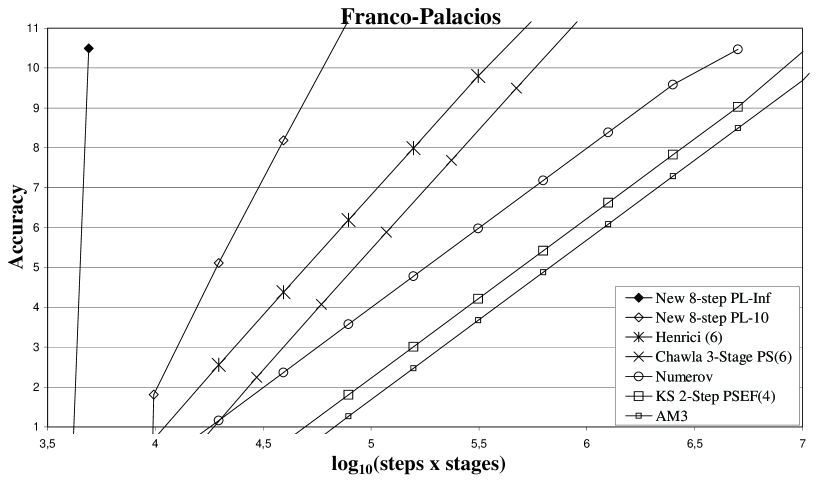
Figure 1: Efficiency for the Orbital Problem by Franco and Palacios

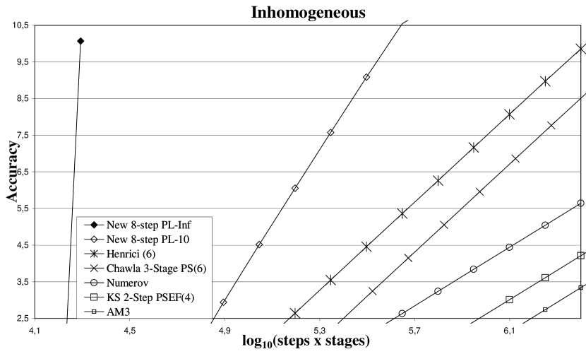
Figure 2: Efficiency for the Inhomogeneous equation

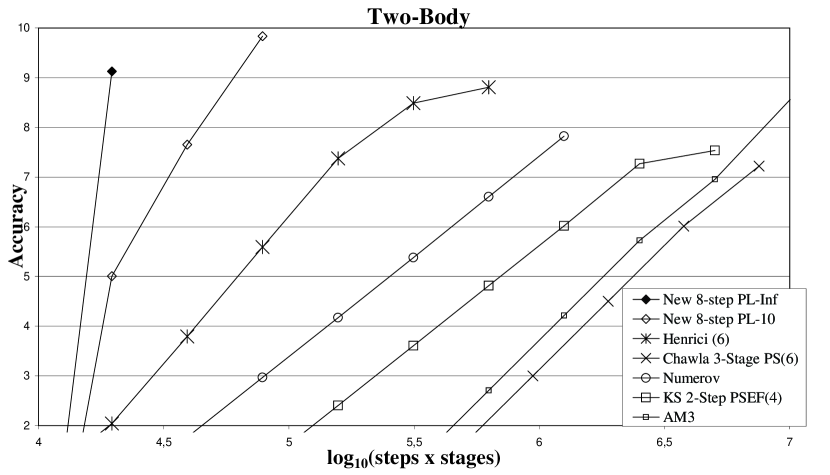
Figure 3: Efficiency for the Two-body problem

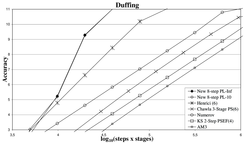
Figure 4: Efficiency for the Duffing equation

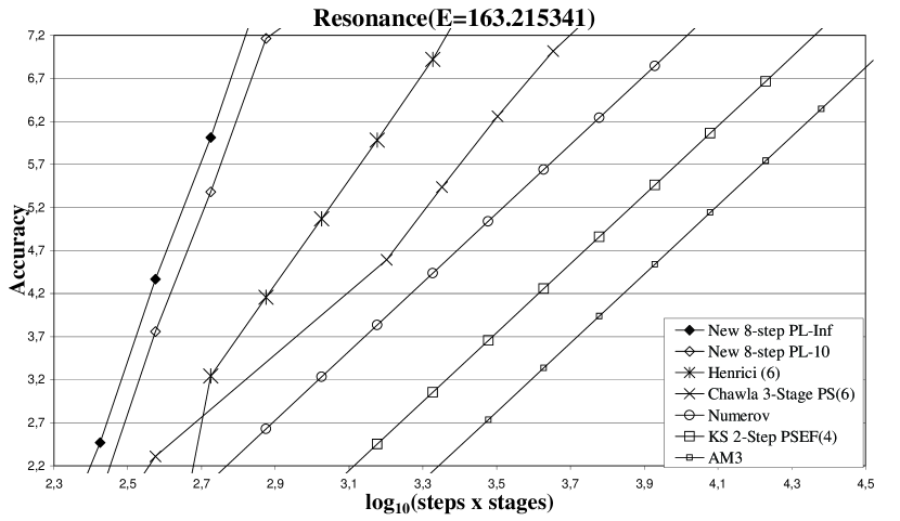
Figure 5: Efficiency for the Schrödinger equation using E = 163.215341

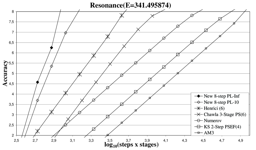
Figure 6: Efficiency for the Schrödinger equation using E = 341.495874

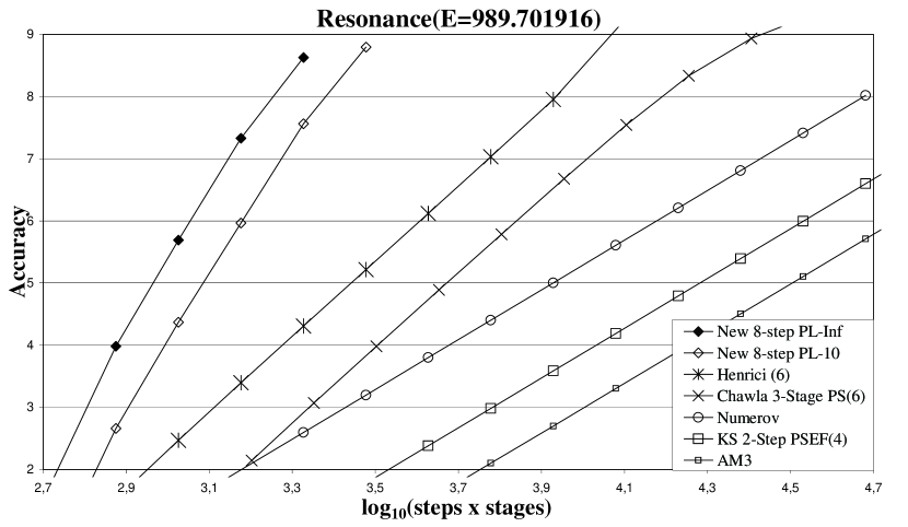
Figure 7: Efficiency for the Schrödinger equation using E = 989.701916

References

- [1] T.E. Simos, Chemical Modelling - Applications and Theory Vol.1, Specialist Periodical Reports, The Royal Society of Chemistry, Cambridge (2000)
- [2] T. Lyche, Chebyshevian multistep methods for Ordinary Differential Eqations, Num. Math. 19, 65-75 (1972)
- [3] M.M. Chawla and P.S. Rao, A Numerov-type method with minimal phase-lag for the integration of second order periodic initial-value problems. II. Explicit method, J.Comput.Appl.Math., 15, 329 (1986)
- [4] P. Henrici, Discrete Variable Methods in Ordinary Diferential Equations, John Wiley and Sons, New York, USA (1962)
- [5] D. Raptis and A.C. Allison, Exponential-fitting methods for the numerical solution of the Schrödinger equation, Computer Physics Communications, 14, 1 (1978)
- [6] Z. Kalogiratou and T.E. Simos, A P-stable exponentially-fitted method for the numerical integration of the Schrödinger equation, Applied Mathematics and Computation, 112, 99-112 (2000)
- [7] L.Gr. Ixaru, M. Rizea, A Numerov-like scheme for the numerical solution of the Schrödinger equation in the deep continuum spectrum of energies, Comp. Phys. Comm. 19, 23-27 (1980)
- [8] J.D. Lambert and I.A. Watson, Symmetric multistep methods for periodic initial values problems, J. Inst. Math. Appl. 18 189 202 (1976)
- [9] J.P. Coleman, L.Gr. Ixaru, P-stability and exponential-fitting methods for , IMA Journal of Numerical Analysis 16, 179-199 (1996)
- [10] J.M. Franco, M. Palacios, J. Comput. Appl. Math., 30, 1 (1990)
- [11] T.E. Simos, P-stable Four-Step Exponentially-Fitted Method for the Numerical Integration of the Schrödinger Equation, CoLe, 1, 1, 37-45 (2005)
- [12] T.E. Simos, Closed Newton-Cotes Trigonometrically-Fitted Formulae for Numerical Integration of the Schrödinger Equation, CoLe, 1, 3, 45-57 (2007)
- [13] Simos TE, A Numerov-Type Method for the Numerical-Solution of the Radial Schrödinger-Equation, Applied Numerical Mathematics, 7, 2, 201-206 (1991)
- [14] Simos TE, Some New 4-Step Exponential-Fitting Methods for The Numerical-Solution of The Radial Schr?dinger-Equation, Ima Journal of Numerical Analysis, 11, 3, 347-356 (1991)
- [15] Simos TE, A High-Order Predictor-Corrector Method for Periodic IVPs, Applied Mathematics Letters, 6, 5, 9-12 (1993)
- [16] L.Gr. Ixaru and M. Micu, Topics in Theoretical Physics. Central Institute of Physics, Bucharest, 1978.
- [17] L.D. Landau and F.M. Lifshitz: Quantum Mechanics. Pergamon, New York, 1965.
- [18] I. Prigogine, Stuart Rice (Eds): Advances in Chemical Physics Vol. 93: New Methods in Computational Quantum Mechanics, John Wiley & Sons, 1997.
- [19] G. Herzberg, Spectra of Diatomic Molecules, Van Nostrand, Toronto, 1950.
- [20] T.E. Simos, Atomic Structure Computations in Chemical Modelling: Applications and Theory (Editor: A. Hinchliffe, UMIST), The Royal Society of Chemistry 38-142(2000).
- [21] T.E. Simos, Numerical methods for 1D, 2D and 3D differential equations arising in chemical problems, Chemical Modelling: Application and Theory, The Royal Society of Chemistry, 2(2002),170-270.
- [22] T.E. Simos and P.S. Williams, On finite difference methods for the solution of the Schrödinger equation, Computers & Chemistry 23 513-554(1999).
- [23] T.E. Simos: Numerical Solution of Ordinary Differential Equations with Periodical Solution. Doctoral Dissertation, National Technical University of Athens, Greece, 1990 (in Greek).
- [24] A. Konguetsof and T.E. Simos, On the Construction of exponentially-fitted methods for the numerical solution of the Schrödinger Equation, Journal of Computational Methods in Sciences and Engineering 1 143-165(2001).
- [25] A.D. Raptis and A.C. Allison: Exponential - fitting methods for the numerical solution of the Schrödinger equation, Computer Physics Communications, 14 1-5(1978).
- [26] A.D. Raptis, Exponential multistep methods for ordinary differential equations, Bull. Greek Math. Soc. 25 113-126(1984).
- [27] L.Gr. Ixaru, Numerical Methods for Differential Equations and Applications, Reidel, Dordrecht - Boston - Lancaster, 1984.
- [28] T. E. Simos, P. S. Williams: A New Runge-Kutta-Nystrom Method with Phase-Lag of Order Infinity for the Numerical Solution of the Schrödinger Equation, MATCH Commun. Math. Comput. Chem. 45 123-137(2002).
- [29] T. E. Simos, Multiderivative Methods for the Numerical Solution of the Schrödinger Equation, MATCH Commun. Math. Comput. Chem. 45 7-26(2004).
- [30] A.D. Raptis, Exponentially-fitted solutions of the eigenvalue Shrödinger equation with automatic error control, Computer Physics Communications, 28 427-431(1983)
- [31] A.D. Raptis, On the numerical solution of the Schrodinger equation, Computer Physics Communications, 24 1-4(1981)
- [32] A.D. Raptis and T.E. Simos, A four-step phase-fitted method for the numerical integration of second order initial-value problem, BIT, 31 160-168(1991).
- [33] M.M. Chawla, Uncoditionally stable Noumerov-type methods for second order differential equations, BIT, 23 541-542(1983).
- [34] M. M. Chawla and P. S. Rao, A Noumerov-type method with minimal phase-lag for the integration of second order periodic initial-value problems, Journal of Computational and Applied Mathematics 11(3) 277-281(1984)
- [35] Liviu Gr. Ixaru and Guido Vanden Berghe, Exponential Fitting, Series on Mathematics and its Applications, Vol. 568, Kluwer Academic Publisher, The Netherlands, 2004.
- [36] L. Gr. Ixaru and M. Rizea, Comparison of some four-step methods for the numerical solution of the Schrödinger equation, Computer Physics Communications, 38(3) 329-337(1985)
- [37] Z.A. Anastassi, T.E. Simos, A family of exponentially-fitted Runge-Kutta methods with exponential order up to three for the numerical solution of the Schrödinger equation, J. Math. Chem 41 (1) 79-100 (2007)
- [38] T. Monovasilis, Z. Kalogiratou , T.E. Simos, Trigonometrically fitted and exponentially fitted symplectic methods for the numerical integration of the Schrödinger equation, J. Math. Chem 40 (3) 257-267 (2006)
- [39] G. Psihoyios, T.E. Simos, The numerical solution of the radial Schrödinger equation via a trigonometrically fitted family of seventh algebraic order Predictor-Corrector methods, J. Math. Chem 40 (3) 269-293 (2006)
- [40] T.E. Simos, A four-step exponentially fitted method for the numerical solution of the Schrödinger equation, J. Math. Chem 40 (3) 305-318 (2006)
- [41] T. Monovasilis, Z. Kalogiratou , T.E. Simos, Exponentially fitted symplectic methods for the numerical integration of the Schrödinger equation J. Math. Chem 37 (3) 263-270 (2005)
- [42] Z. Kalogiratou , T. Monovasilis, T.E. Simos, Numerical solution of the two-dimensional time independent Schrödinger equation with Numerov-type methods J. Math. Chem 37 (3) 271-279 (2005)
- [43] Z.A. Anastassi, T.E. Simos, Trigonometrically fitted Runge-Kutta methods for the numerical solution of the Schrödinger equation J. Math. Chem 37 (3) 281-293 (2005)
- [44] G. Psihoyios, T.E. Simos, Sixth algebraic order trigonometrically fitted predictor-corrector methods for the numerical solution of the radial Schrödinger equation, J. Math. Chem 37 (3) 295-316 (2005)
- [45] D.P. Sakas, T.E. Simos, A family of multiderivative methods for the numerical solution of the Schrödinger equation, J. Math. Chem 37 (3) 317-331 (2005)
- [46] T.E. Simos, Exponentially - fitted multiderivative methods for the numerical solution of the Schrödinger equation, J. Math. Chem 36 (1) 13-27 (2004)
- [47] K. Tselios, T.E. Simos, Symplectic methods of fifth order for the numerical solution of the radial Shrodinger equation, J. Math. Chem 35 (1) 55-63 (2004)
- [48] T.E. Simos, A family of trigonometrically-fitted symmetric methods for the efficient solution of the Schrödinger equation and related problems J. Math. Chem 34 (1-2) 39-58 JUL 2003
- [49] K. Tselios, T.E. Simos, Symplectic methods for the numerical solution of the radial Shrödinger equation, J. Math. Chem 34 (1-2) 83-94 (2003)
- [50] J. Vigo-Aguiar J, T.E. Simos, Family of twelve steps exponential fitting symmetric multistep methods for the numerical solution of the Schrödinger equation, J. Math. Chem 32 (3) 257-270 (2002)
- [51] G. Avdelas, E. Kefalidis, T.E. Simos, New P-stable eighth algebraic order exponentially-fitted methods for the numerical integration of the Schrödinger equation, J. Math. Chem 31 (4) 371-404 (2002)
- [52] T.E. Simos, J. Vigo-Aguiar, Symmetric eighth algebraic order methods with minimal phase-lag for the numerical solution of the Schrödinger equation J. Math. Chem 31 (2) 135-144 (2002)
- [53] Z. Kalogiratou , T.E. Simos, Construction of trigonometrically and exponentially fitted Runge-Kutta-Nystrom methods for the numerical solution of the Schrödinger equation and related problems a method of 8th algebraic order, J. Math. Chem 31 (2) 211-232
- [54] T.E. Simos, J. Vigo-Aguiar, A modified phase-fitted Runge-Kutta method for the numerical solution of the Schrödinger equation, J. Math. Chem 30 (1) 121-131 (2001)
- [55] G. Avdelas, A. Konguetsof, T.E. Simos, A generator and an optimized generator of high-order hybrid explicit methods for the numerical solution of the Schrödinger equation. Part 1. Development of the basic method, J. Math. Chem 29 (4) 281-291 (2001)
- [56] G. Avdelas, A. Konguetsof, T.E. Simos, A generator and an optimized generator of high-order hybrid explicit methods for the numerical solution of the Schrödinger equation. Part 2. Development of the generator; optimization of the generator and numerical results, J. Math. Chem 29 (4) 293-305 (2001)
- [57] J. Vigo-Aguiar, T.E. Simos, A family of P-stable eighth algebraic order methods with exponential fitting facilities, J. Math. Chem 29 (3) 177-189 (2001)
- [58] T.E. Simos, A new explicit Bessel and Neumann fitted eighth algebraic order method for the numerical solution of the Schrödinger equation J. Math. Chem 27 (4) 343-356 (2000)
- [59] G. Avdelas, T.E. Simos, Embedded eighth order methods for the numerical solution of the Schrödinger equation, J. Math. Chem 26 (4) 327-341 1999,
- [60] T.E. Simos, A family of P-stable exponentially-fitted methods for the numerical solution of the Schrödinger equation, J. Math. Chem 25 (1) 65-84 (1999)
- [61] T.E. Simos, Some embedded modified Runge-Kutta methods for the numerical solution of some specific Schrödinger equations, J. Math. Chem 24 (1-3) 23-37 (1998)
- [62] T.E. Simos, Eighth order methods with minimal phase-lag for accurate computations for the elastic scattering phase-shift problem, J. Math. Chem 21 (4) 359-372 (1997)
- [63] P. Amodio, I. Gladwell and G. Romanazzi, Numerical Solution of General Bordered ABD Linear Systems by Cyclic Reduction, JNAIAM J. Numer. Anal. Indust. Appl. Math 1(1) 5-12(2006)
- [64] S. D. Capper, J. R. Cash and D. R. Moore, Lobatto-Obrechkoff Formulae for 2nd Order Two-Point Boundary Value Problems, JNAIAM J. Numer. Anal. Indust. Appl. Math 1(1) 13-25 (2006)
- [65] S. D. Capper and D. R. Moore, On High Order MIRK Schemes and Hermite-Birkhoff Interpolants, JNAIAM J. Numer. Anal. Indust. Appl. Math 1(1) 27-47 (2006)
- [66] J. R. Cash, N. Sumarti, T. J. Abdulla and I. Vieira, The Derivation of Interpolants for Nonlinear Two-Point Boundary Value Problems, JNAIAM J. Numer. Anal. Indust. Appl. Math 1(1) 49-58 (2006)
- [67] J. R. Cash and S. Girdlestone, Variable Step Runge-Kutta-Nystr m Methods for the Numerical Solution of Reversible Systems, JNAIAM J. Numer. Anal. Indust. Appl. Math 1(1) 59-80 (2006)
- [68] Jeff R. Cash and Francesca Mazzia, Hybrid Mesh Selection Algorithms Based on Conditioning for Two-Point Boundary Value Problems, JNAIAM J. Numer. Anal. Indust. Appl. Math 1(1) 81-90 (2006)
- [69] Felice Iavernaro, Francesca Mazzia and Donato Trigiante, Stability and Conditioning in Numerical Analysis, JNAIAM J. Numer. Anal. Indust. Appl. Math 1(1) 91-112 (2006)
- [70] Felice Iavernaro and Donato Trigiante, Discrete Conservative Vector Fields Induced by the Trapezoidal Method, JNAIAM J. Numer. Anal. Indust. Appl. Math 1(1) 113-130 (2006)
- [71] Francesca Mazzia, Alessandra Sestini and Donato Trigiante, BS Linear Multistep Methods on Non-uniform Meshes, JNAIAM J. Numer. Anal. Indust. Appl. Math 1(1) 131-144 (2006)
- [72] L.F. Shampine, P.H. Muir, H. Xu, A User-Friendly Fortran BVP Solver, JNAIAM J. Numer. Anal. Indust. Appl. Math 1(2) 201-217 (2006)
- [73] G. Vanden Berghe and M. Van Daele, Exponentially- fitted St rmer/Verlet methods, JNAIAM J. Numer. Anal. Indust. Appl. Math 1(3) 241-255 (2006)
- [74] L. Aceto, R. Pandolfi, D. Trigiante, Stability Analysis of Linear Multistep Methods via Polynomial Type Variation, JNAIAM J. Numer. Anal. Indust. Appl. Math 2(1-2) 1-9 (2007)
- [75] G. Psihoyios, A Block Implicit Advanced Step-point (BIAS) Algorithm for Stiff Differential Systems, Computing Letters 2(1-2) 51-58(2006)
- [76] W.H. Enright, On the use of ’arc length’ and ’defect’ for mesh selection for differential equations, Computing Letters 1(2) 47-52(2005)
- [77] T.E. Simos, Stabilization of a Four-Step Exponentially-Fitted Method and its Application to the Schrödinger Equation, International Journal of Modern Physics C 18(3) 315-328(2007).
- [78] Zhongcheng Wang, P-stable linear symmetric multistep methods for periodic initial-value problems, Computer Physics Communications 171 162 174(2005)
- [79] T.E. Simos, A Runge-Kutta Fehlberg method with phase-lag of order infinity for initial value problems with oscillating solution, Computers and Mathematics with Applications 25 95-101(1993).
- [80] T.E. Simos, Runge-Kutta interpolants with minimal phase-lag, Computers and Mathematics with Applications 26 43-49(1993).
- [81] T.E. Simos, Runge-Kutta-Nyström interpolants for the numerical integration of special second-order periodic initial-value problems, Computers and Mathematics with Applications 26 7-15(1993).
- [82] T.E. Simos and G.V. Mitsou, A family of four-step exponential fitted methods for the numerical integration of the radial Schrödinger equation, Computers and Mathematics with Applications 28 41-50(1994).
- [83] T.E. Simos and G. Mousadis, A two-step method for the numerical solution of the radial Schr dinger equation, Computers and Mathematics with Applications 29 31-37(1995).
- [84] G. Avdelas and T.E. Simos, Block Runge-Kutta methods for periodic initial-value problems, Computers and Mathematics with Applications 31 69- 83(1996).
- [85] G. Avdelas and T.E. Simos, Embedded methods for the numerical solution of the Schrödinger equation, Computers and Mathematics with Applications 31 85-102(1996).
- [86] G. Papakaliatakis and T.E. Simos, A new method for the numerical solution of fourth order BVP s with oscillating solutions, Computers and Mathematics with Applications 32 1-6(1996).
- [87] T.E. Simos, An extended Numerov-type method for the numerical solution of the Schrödinger equation, Computers and Mathematics with Applications 33 67-78(1997).
- [88] T.E. Simos, A new hybrid imbedded variable-step procedure for the numerical integration of the Schrödinger equation, Computers and Mathematics with Applications 36 51-63(1998).
- [89] T.E. Simos, Bessel and Neumann Fitted Methods for the Numerical Solution of the Schrödinger equation, Computers & Mathematics with Applications 42 833-847(2001).
- [90] A. Konguetsof and T.E. Simos, An exponentially-fitted and trigonometrically-fitted method for the numerical solution of periodic initial-value problems, Computers and Mathematics with Applications 45 547-554(2003).
- [91] Z.A. Anastassi and T.E. Simos, An optimized Runge-Kutta method for the solution of orbital problems, Journal of Computational and Applied Mathematics 175(1) 1-9(2005)
- [92] G. Psihoyios and T.E. Simos, A fourth algebraic order trigonometrically fitted predictor-corrector scheme for IVPs with oscillating solutions, Journal of Computational and Applied Mathematics 175(1) 137-147(2005)
- [93] D.P. Sakas and T.E. Simos, Multiderivative methods of eighth algrebraic order with minimal phase-lag for the numerical solution of the radial Schrödinger equation, Journal of Computational and Applied Mathematics 175(1) 161-172(2005)
- [94] K. Tselios and T.E. Simos, Runge-Kutta methods with minimal dispersion and dissipation for problems arising from computational acoustics, Journal of Computational and Applied Mathematics 175(1) 173-181(2005)
- [95] Z. Kalogiratou and T.E. Simos, Newton-Cotes formulae for long-time integration, Journal of Computational and Applied Mathematics 158(1) 75-82(2003)
- [96] Z. Kalogiratou, T. Monovasilis and T.E. Simos, Symplectic integrators for the numerical solution of the Schrödinger equation, Journal of Computational and Applied Mathematics 158(1) 83-92(2003)
- [97] A. Konguetsof and T.E. Simos, A generator of hybrid symmetric four-step methods for the numerical solution of the Schrödinger equation, Journal of Computational and Applied Mathematics 158(1) 93-106(2003)
- [98] G. Psihoyios and T.E. Simos, Trigonometrically fitted predictor-corrector methods for IVPs with oscillating solutions, Journal of Computational and Applied Mathematics 158(1) 135-144(2003)
- [99] Ch. Tsitouras and T.E. Simos, Optimized Runge-Kutta pairs for problems with oscillating solutions, Journal of Computational and Applied Mathematics 147(2) 397-409(2002)
- [100] T.E. Simos, An exponentially fitted eighth-order method for the numerical solution of the Schrödinger equation, Journal of Computational and Applied Mathematics 108(1-2) 177-194(1999)
- [101] T.E. Simos, An accurate finite difference method for the numerical solution of the Schrödinger equation, Journal of Computational and Applied Mathematics 91(1) 47-61(1998)
- [102] R.M. Thomas and T.E. Simos, A family of hybrid exponentially fitted predictor-corrector methods for the numerical integration of the radial Schrödinger equation, Journal of Computational and Applied Mathematics 87(2) 215-226(1997)
- [103] Z.A. Anastassi and T.E. Simos: Special Optimized Runge-Kutta methods for IVPs with Oscillating Solutions, International Journal of Modern Physics C, 15, 1-15 (2004)
- [104] Z.A. Anastassi and T.E. Simos: A Dispersive-Fitted and Dissipative-Fitted Explicit Runge-Kutta method for the Numerical Solution of Orbital Problems, New Astronomy, 10, 31-37 (2004)
- [105] Z.A. Anastassi and T.E. Simos: A Trigonometrically-Fitted Runge-Kutta Method for the Numerical Solution of Orbital Problems, New Astronomy, 10, 301-309 (2005)
- [106] T.V. Triantafyllidis, Z.A. Anastassi and T.E. Simos: Two Optimized Runge-Kutta Methods for the Solution of the Schr?dinger Equation, MATCH Commun. Math. Comput. Chem., 60, 3 (2008)
- [107] Z.A. Anastassi and T.E. Simos, Trigonometrically Fitted Fifth Order Runge-Kutta Methods for the Numerical Solution of the Schrödinger Equation, Mathematical and Computer Modelling, 42 (7-8), 877-886 (2005)
- [108] Z.A. Anastassi and T.E. Simos: New Trigonometrically Fitted Six-Step Symmetric Methods for the Efficient Solution of the Schrödinger Equation, MATCH Commun. Math. Comput. Chem., 60, 3 (2008)
- [109] G.A. Panopoulos, Z.A. Anastassi and T.E. Simos: Two New Optimized Eight-Step Symmetric Methods for the Efficient Solution of the Schrödinger Equation and Related Problems, MATCH Commun. Math. Comput. Chem., 60, 3 (2008)
- [110] Z.A. Anastassi and T.E. Simos: A Six-Step P-stable Trigonometrically-Fitted Method for the Numerical Integration of the Radial Schrödinger Equation, MATCH Commun. Math. Comput. Chem., 60, 3 (2008)
- [111] Z.A. Anastassi and T.E. Simos, A family of two-stage two-step methods for the numerical integration of the Schrödinger equation and related IVPs with oscillating solution, Journal of Mathematical Chemistry, Article in Press, Corrected Proof
- [112] T.E. Simos and P.S. Williams, A finite-difference method for the numerical solution of the Schrödinger equation, Journal of Computational and Applied Mathematics 79(2) 189-205(1997)
- [113] G. Avdelas and T.E. Simos, A generator of high-order embedded P-stable methods for the numerical solution of the Schrödinger equation, Journal of Computational and Applied Mathematics 72(2) 345-358(1996)
- [114] R.M. Thomas, T.E. Simos and G.V. Mitsou, A family of Numerov-type exponentially fitted predictor-corrector methods for the numerical integration of the radial Schrödinger equation, Journal of Computational and Applied Mathematics 67(2) 255-270(1996)
- [115] T.E. Simos, A Family of 4-Step Exponentially Fitted Predictor-Corrector Methods for the Numerical-Integration of The Schrödinger-Equation, Journal of Computational and Applied Mathematics 58(3) 337-344(1995)
- [116] T.E. Simos, An Explicit 4-Step Phase-Fitted Method for the Numerical-Integration of 2nd-order Initial-Value Problems, Journal of Computational and Applied Mathematics 55(2) 125-133(1994)
- [117] T.E. Simos, E. Dimas and A.B. Sideridis, A Runge-Kutta-Nyström Method for the Numerical-Integration of Special 2nd-order Periodic Initial-Value Problems, Journal of Computational and Applied Mathematics 51(3) 317-326(1994)
- [118] A.B. Sideridis and T.E. Simos, A Low-Order Embedded Runge-Kutta Method for Periodic Initial-Value Problems, Journal of Computational and Applied Mathematics 44(2) 235-244(1992)
- [119] T.E. Simos amd A.D. Raptis, A 4th-order Bessel Fitting Method for the Numerical-Solution of the SchrÖdinger-Equation, Journal of Computational and Applied Mathematics 43(3) 313-322(1992)
- [120] T.E. Simos, Explicit 2-Step Methods with Minimal Phase-Lag for the Numerical-Integration of Special 2nd-order Initial-Value Problems and their Application to the One-Dimensional Schrödinger-Equation, Journal of Computational and Applied Mathematics 39(1) 89-94(1992)
- [121] T.E. Simos, A 4-Step Method for the Numerical-Solution of the Schrödinger-Equation, Journal of Computational and Applied Mathematics 30(3) 251-255(1990)
- [122] C.D. Papageorgiou, A.D. Raptis and T.E. Simos, A Method for Computing Phase-Shifts for Scattering, Journal of Computational and Applied Mathematics 29(1) 61-67(1990)
- [123] A.D. Raptis, Two-Step Methods for the Numerical Solution of the Schrödinger Equation, Computing 28 373-378(1982).
- [124] T.E. Simos. A new Numerov-type method for computing eigenvalues and resonances of the radial Schrödinger equation, International Journal of Modern Physics C-Physics and Computers, 7(1) 33-41(1996)
- [125] T.E. Simos, Predictor Corrector Phase-Fitted Methods for Y”=F(X,Y) and an Application to the Schrödinger-Equation, International Journal of Quantum Chemistry, 53(5) 473-483(1995)
- [126] T.E. Simos, Two-step almost P-stable complete in phase methods for the numerical integration of second order periodic initial-value problems, Inter. J. Comput. Math. 46 77-85(1992).
- [127] R. M. Corless, A. Shakoori, D.A. Aruliah, L. Gonzalez-Vega, Barycentric Hermite Interpolants for Event Location in Initial-Value Problems, JNAIAM J. Numer. Anal. Indust. Appl. Math, 3, 1-16 (2008)
- [128] M. Dewar, Embedding a General-Purpose Numerical Library in an Interactive Environment, JNAIAM J. Numer. Anal. Indust. Appl. Math, 3, 17-26 (2008)
- [129] J. Kierzenka and L.F. Shampine, A BVP Solver that Controls Residual and Error, JNAIAM J. Numer. Anal. Indust. Appl. Math, 3, 27-41 (2008)
- [130] R. Knapp, A Method of Lines Framework in Mathematica, JNAIAM J. Numer. Anal. Indust. Appl. Math, 3, 43-59 (2008)
- [131] N. S. Nedialkov and J. D. Pryce, Solving Differential Algebraic Equations by Taylor Series (III): the DAETS Code, JNAIAM J. Numer. Anal. Indust. Appl. Math, 3, 61-80 (2008)
- [132] R. L. Lipsman, J. E. Osborn, and J. M. Rosenberg, The SCHOL Project at the University of Maryland: Using Mathematical Software in the Teaching of Sophomore Differential Equations, JNAIAM J. Numer. Anal. Indust. Appl. Math, 3, 81-103 (2008)
- [133] M. Sofroniou and G. Spaletta, Extrapolation Methods in Mathematica, JNAIAM J. Numer. Anal. Indust. Appl. Math, 3, 105-121 (2008)
- [134] R. J. Spiteri and Thian-Peng Ter, pythNon: A PSE for the Numerical Solution of Nonlinear Algebraic Equations, JNAIAM J. Numer. Anal. Indust. Appl. Math, 3, 123-137 (2008)
- [135] S.P. Corwin, S. Thompson and S.M. White, Solving ODEs and DDEs with Impulses, JNAIAM J. Numer. Anal. Indust. Appl. Math, 3, 139-149 (2008)
- [136] W. Weckesser, VFGEN: A Code Generation Tool, JNAIAM J. Numer. Anal. Indust. Appl. Math, 3, 151-165 (2008)
- [137] A. Wittkopf, Automatic Code Generation and Optimization in Maple, JNAIAM J. Numer. Anal. Indust. Appl. Math, 3, 167-180 (2008)