GLOBAL SLIM ACCRETION DISK SOLUTIONS REVISITED

Abstract

We show that there exists a maximal possible accretion rate, beyond which global slim disk solutions cannot be constructed because in the vertical direction the gravitational force would be unable to balance the pressure force to gather the accreted matter. The principle for this restriction is the same as that for the Eddington luminosity and the corresponding critical accretion rate, which were derived for spherical accretion by considering the same force balance in the radial direction. If the assumption of hydrostatic equilibrium is waived and vertical motion is included, this restriction may become even more serious as the value of the maximal possible accretion rate becomes smaller. Previous understanding in the literature that global slim disk solutions could stand for any large accretion rates is due to the overestimation of the vertical gravitational force by using an approximate potential. For accretion flows with large accretion rates at large radii, outflows seem unavoidable in order for the accretion flow to reduce the accretion rate and follow a global solution till the central black hole.

1 INTRODUCTION

Although great progress has been made in recent years in increasingly sophisticated numerical accretion disk simulations, simple analytic disk models still are the only accessible way of making direct link between the theory and observations, as only these models can be used to estimate, e.g., the spectra of accretion-powered astrophysical systems. This fact justifies the continuous effort to improve the understanding of accretion processes using a simple viscosity parameterization.

The slim disk model is one of such simple analytic models for black hole accretion (Abramowicz et al. 1988; Kato et al. 1998). This model was developed upon the standard Shakura-Sunyaev disk (SSD) model (Shakura & Sunyaev 1973) by considering two processes in black hole accretion flows, namely the transonic motion and the advective heat transport, which were neglected in the SSD model. In the limit of low mass accretion rates, i.e., $\dot{M}$ is substantially lower than its critical value $\dot{M}_{\mathrm{Edd}}$ corresponding to the Eddington luminosity $L_{\mathrm{Edd}}$, say, $\dot{M}\lesssim 0.1\dot{M}_{\mathrm{Edd}}$, the advective heat transport is unimportant, and the structure of slim disks is similar to that of SSDs, with a difference that slim disk flows are transonic in their inner regions (e.g., Chen & Taam 1993). In this sense, the theoretical basis of black hole disk models for low and even moderate accretion rates is well established. But the slim disk model is supposed to have the advantage over the SSD model that it can be extended to the case of high accretion rates, i.e., with $\dot{M}$ approaching or surpassing $\dot{M}_{\mathrm{Edd}}$. In this case, the very basic assumption of the SSD model that is valid only for low accretion rates, i.e., the geometrical thinness, $H\ll r$, where $H$ is the half-thickness of the disk and $r$ is the cylindrical radius, would break down (Frank et al. 2002, p. 98). It was then suggested in the slim disk model that the disk becomes geometrically slim, i.e., with $H\lesssim r$; and accordingly, the process of advective heat transport becomes important or even dominant over the radiative cooling because, as given by Abramowicz et al. (1986), there is a relation $f_{\mathrm{adv}}\varpropto(H/r)^{2}$, where $f_{\mathrm{adv}}\equiv Q_{\mathrm{adv}}^{-}/Q_{\mathrm{vis}}^{+}$ is the advective factor, with $Q_{\mathrm{adv}}^{-}$ and $Q_{\mathrm{vis}}^{+}$ being the advective cooling and viscous heating rates per unit area of the disk, respectively.

However, the self-consistency of the slim disk model and its applicability to the high accretion rate case are not so obvious. In particular, uncertainties seem to concentrate on the treatment of the vertical structure of the disk. First, vertical hydrostatic equilibrium is a reasonable assumption for SSDs because, for geometrically thin disks, vertical motion of the disk matter must be negligible compared with radial motion; but it is questionable to adopt this assumption for slim disks that are not thin. Second, as noticed recently by Gu & Lu (2007, hereafter GL07), even the vertical hydrostatic equilibrium is assumed, in the slim disk model there is a serious inconsistency that the vertical gravitational force was greatly magnified by using the approximate form of potential due to Hōshi (1977), which is valid only for thin disks again; and accordingly, the previous understanding that slim disks could exist for any large accretion rates seems doubtful. Third, the above mentioned relation $f_{\mathrm{adv}}\varpropto(H/r)^{2}$ was derived with the Hōshi approximation of potential, so its applicability to not thin disks with large accretion rates is not justified; or in other words, it is not clear whether an accretion disk can ensure advection dominance (i.e., $f_{\mathrm{adv}}>0.5$) while remaining to be geometrically slim. According to the analyses of Narayan & Yi (1995) and Gu et al. (2008), in order for advection to be dominant, the disk needs to be geometrically thick, i.e., with $H>r$, rather than slim. This is probably the reason why $H>r$ was obtained in many numerical calculations of slim disks and other accretion disks (see references in GL07).

What about another popular black hole accretion disk model, the advection-dominated accretion flow (ADAF) model (Narayan & Yi 1994; Abramowicz et al. 1995)? ADAFs are also supposed to be geometrically slim and advection-dominated, and their vertical structure was treated in a way similar to that for slim disks. The above mentioned uncertainties should also apply to the ADAF model, because they are based on purely hydrostatic considerations and are related only to the geometrical thickness of the disk. Many two- and three-dimensional numerical simulations of viscous radiatively inefficient accretion flows revealed the existence of convection-dominated accretion flows rather than ADAFs (see references in GL07). This fact is probably an indication that the ADAF model might have hidden inconsistencies, and one of which might be related to the treatment of vertical structure. What is different from slim disks is that ADAFs are expected to correspond to very low accretion rates and are known to have a maximal possible accretion rate at each radius (e.g., Abramowicz et al. 1995), so the problem addressed in GL07 regarding the allowed accretion rate may have no impact on ADAFs. In addition, ADAFs are optically thin and ion pressure-supported, the radiation processes in them are more complicated, making the vertical structure more difficult to deal with, than for slim disks that are optically thick and radiation pressure-supported.

Our present work is devoted to discuss the slim disk model and is a straightforward continuation of GL07. All the results of GL07 were based on a local analysis, i.e., only for a certain radius. Although a similar local analysis was often used in the literature (e.g., Abramowicz et al. 1995; Chen et al. 1995; Kato et al. 1998), one should be cautious of the fact that conclusions made in the local sense do not necessarily hold in the global sense. For example, it has been shown that, even though a disk is locally unstable at a given radius according to a local stability analysis, the disk can be globally stable in global numerical simulations (Janiuk et al. 2002; Gierliński & Done 2004). Therefore, it is worthwhile to check and extend the results of GL07 by investigating global solutions of original differential equations for black hole accretion flows, similar to what was done by, e.g., Chen & Wang (2004), Watarai et al. (2005), Artemova et al. (2006), and Watarai (2006), but with a revised vertical gravitational force.

2 SOLUTIONS WITH VERTICAL HYDROSTATIC EQUILIBRIUM

2.1 Equations

The basic equations to be solved for slim disks can be written in cylindrical coordinates as (cf. Kato et al. 1998, p. 236; GL07):

$$\dot{M}=-2\pi r\Sigma v_{r}={\mathrm{constant}},$$ (1)

$$v_{r}\frac{dv_{r}}{dr}+\frac{1}{\rho_{0}}\frac{dp_{0}}{dr}+(\Omega_{\mathrm{K}}^{2}-\Omega^{2})r=0,$$ (2)

$$\dot{M}(\Omega r^{2}-j)=2\pi\alpha r^{2}\Pi,$$ (3)

$$Q_{\mathrm{vis}}^{+}=Q_{\mathrm{adv}}^{-}+Q_{\mathrm{rad}}^{-},$$ (4)

$$p_{0}=\frac{k_{\mathrm{B}}\rho_{0}T_{0}}{\mu m_{p}}+\frac{1}{3}aT^{4}_{0},$$ (5)

where $\Sigma=2\int_{0}^{H}\rho dz$ is the surface density, $\rho$ is the density, $p$ is the pressure, $v_{r}$ is the radial velocity, $\Omega$ is the angular velocity and $\Omega_{\mathrm{K}}$ is its Keplerian value, $j$ is an integration constant representing the specific angular momentum accreted by the black hole, $\alpha$ is the Shakura-Sunyaev viscosity parameter, $\Pi=2\int_{0}^{H}pdz$ is the vertically integrated pressure, $Q_{\mathrm{rad}}^{-}$ is the radiative cooling rate per unit area, $T$ is the temperature, $\mu$ is the mean molecular weight and is taken to be 0.62, and the subscript “0” represents quantities on the equatorial plane.

There are some differences between equations (1 - 5) and the basic equations in GL07 (their eqs. [6 - 10]). In GL07 all the five equations were written in the vertically integrated form; here the continuity equations (1), angular momentum equation (3), and energy equation (4) are in the same form, because it is obviously convenient to write equation (1) in this form and equations (3) and (4) also contain $\dot{M}$; but the radial momentum equation (2) and state equation (5) are given for equatorial quantities. The state equation of GL07 (their eq. [10]) is a trivial vertical integration of our equation (5) and makes no difference. But in GL07 (and also in Kato et al. 1998), in obtaining the vertically integrated radial momentum equation (eq. [7] of GL07 or eq. [8.25] of Kato et al. 1998), some simplifications were made. First, both $v_{r}$ and $\Omega$ were regarded to be independent of the coordinate $z$, and this is also adopted in our equations here. Second, a step $\int_{-H}^{H}\frac{dp}{dr}dz=\frac{d\Pi}{dr}$ was taken, but in the strict sense this equality holds only when $H$ does not vary with $r$, in studies of global solutions here we should better not to take it. This is the reason why we prefer to write equation (2) for equatorial quantities. The differential equation (4) was reduced to be an algebraic one in GL07; and here instead, it keeps its original form with the explicit expressions for $Q_{\mathrm{vis}}^{+}$, $Q_{\mathrm{adv}}^{-}$, and $Q_{\mathrm{rad}}^{-}$ given as

$$Q_{\mathrm{vis}}^{+}=-\frac{\dot{M}\Omega(\Omega r^{2}-j)}{2\pi r^{2}}\frac{d\ln{\Omega}}{d\ln{r}},$$ (6)

$$Q_{\mathrm{adv}}^{-}=-\frac{3\dot{M}}{2\pi r^{2}}\frac{\Pi}{\Sigma}\left(\frac{d\ln p_{0}}{d\ln r}-\frac{4}{3}\frac{d\ln\rho_{0}}{d\ln r}\right),$$ (7)

$$Q_{\mathrm{rad}}^{-}=\frac{32\sigma T_{0}^{4}}{3\overline{\kappa}\rho_{0}H}$$ (8)

(Kato et al. 1998), where $\overline{\kappa}=\kappa_{{\mathrm{es}}}+\kappa_{{\mathrm{ff}}}=0.34+6.4\times{10^{22}}\overline{\rho}\overline{T}^{\ -7/2}\mathrm{cm^{2}\ g^{-1}}$, $\overline{\rho}(=\Sigma/2H)$ and $\overline{T}(=\int_{0}^{H}Tdz/H)$ are the vertically averaged density and temperature, respectively.

The key difference between the existing slim disk model and our work here is in the treatment of the vertical hydrostatic equilibrium equation,

$$\frac{\partial p}{\partial z}+\rho\frac{\partial\psi}{\partial z}=0,$$ (9)

where $\psi$ is the potential. In the slim disk model (e.g., Kato et al. 1998, p. 241), the potential of Paczyński & Wiita (1980),

$$\psi(r,z)=-\frac{GM}{\sqrt{r^{2}+z^{2}}-r_{g}},$$ (10)

where $r_{g}\equiv 2GM/c^{2}$ is the gravitational radius, was approximated in the form of Hōshi (1977), i.e.,

$$\psi(r,z)\approx\psi(r,0)+\frac{\Omega_{\mathrm{K}}^{2}z^{2}}{2}.$$ (11)

Using equation (11) and assuming a polytropic relation in the vertical direction, $p=K\rho^{1+1/N}$, where $K$ and $N$ are constants, the vertical integration of equation (9) gave (for $N=3$)

$$\left(\frac{\rho}{\rho_{0}}\right)^{1/3}=\left(\frac{p}{p_{0}}\right)^{1/4}=\frac{T}{T_{0}}=1-\frac{z^{2}}{H^{2}},$$ (12)

$$8\frac{p_{0}}{\rho_{0}}=\Omega_{\mathrm{K}}^{2}H^{2},$$ (13)

and $\Sigma$ and $\Pi$ were

$$\Sigma=2\times\frac{16}{35}\rho_{0}H,$$ (14)

$$\Pi=2\times\frac{128}{315}p_{0}H.$$ (15)

The simple relation ${c_{s}}/\Omega_{\mathrm{K}}H=\mathrm{constant}$ was obtained, with the sound speed $c_{s}$ being defined either as $c_{s}^{2}=p_{0}/\rho_{0}$ or as $c_{s}^{2}=\Pi/\Sigma$.

However, as the main point made in GL07, the approximation of equation (11) is invalid for slim disks. By using the explicit Paczyński & Wiita potential, equation (10), to integrate equation (9), one obtains instead of equations (12) and (13):

$$g=\left(\frac{\rho}{\rho_{0}}\right)^{1/3}=\left(\frac{p}{p_{0}}\right)^{1/4}=\frac{T}{T_{0}}=\frac{\frac{1}{\sqrt{r^{2}+z^{2}}-r_{g}}-\frac{1}{\sqrt{r^{2}+H^{2}}-r_{g}}}{\frac{1}{r-r_{g}}-\frac{1}{\sqrt{r^{2}+H^{2}}-r_{g}}},$$ (16)

$$4\frac{p_{0}}{\rho_{0}}=GM\left(\frac{1}{r-r_{g}}-\frac{1}{\sqrt{r^{2}+H^{2}}-r_{g}}\right).$$ (17)

Accordingly, $\Sigma$ and $\Pi$ become

$$\Sigma=2\rho_{0}\int_{0}^{H}g^{3}dz,$$ (18)

$$\Pi=2p_{0}\int_{0}^{H}g^{4}dz,$$ (19)

which are much more complicated than equations (14) and (15). It is seen that the relation ${c_{s}}/\Omega_{\mathrm{K}}H=\mathrm{constant}$ does not hold.

To summarize, in the existing slim disk model, the set of eight equations, namely equations (1 - 5) and (13 - 15), could be solved for the eight unknown quantities $\rho_{0}$, $p_{0}$, $\Sigma$, $\Pi$, $T_{0}$, $v_{r}$, $\Omega$, and $H$ as functions of $r$, with given constant parameters $M$, $\dot{M}$, $\alpha$, and $j$; while in our work here, equations (17 - 19), instead of equations (13 - 15), still along with equations (1 - 5) form a new set to be solved for the same eight unknowns. There are two differential equations, i.e., equations (2) and (4); and other equations in each set are algebraic, including equations (18) and (19) once the vertical integration is analytically made.

2.2 Solutions

We numerically solve the set of equations (1 - 5) and (17 - 19), i.e., with the correctly calculated vertical gravitational force using the explicit Paczyński & Wiita potential. For comparisons, we also solve the set of equations (1 - 5) and (13 - 15), as done already in the existing slim disk model, i.e., with the magnified vertical gravitational force using the Hōshi approximation of the Paczyński & Wiita potential. After some algebra, the equations in each set can be combined into only two differential equations. A physically acceptable global solution should be able to extend from a large radius to the vicinity of the central black hole, passing the sonic point regularly. We start the integration at $r=10^{6}r_{g}$, where the outer boundary conditions are set to be corresponding to an SSD, i.e., being geometrically thin and Keplerian rotating. If a solution is found to be transonic, we extend it to $r=2r_{g}$ (in the following figures only a smaller radial range is shown in order to see more clearly the solution behavior in the inner region). We fix $M=10M_{\sun}$ and $\alpha=0.1$, and vary the values of $\dot{M}$ for different solutions. For a transonic solution, the other constant parameter $j$ is an eigenvalue of the problem and has to be adjusted correctly and accurately (e.g., Chen & Taam 1993; Chen & Wang 2004).

Rather than showing the radial variation of every physical quantity, our main purpose here is to see how the correction of the vertical gravitational force changes the previous understanding of global slim disk solutions, that is, there was no upper limit of $\dot{M}$ for slim disks, any large value of $\dot{M}$ could correspond to a global solution (e.g., Kato et al. 1998; Chen & Wang 2004; Watarai et al. 2005; Watarai 2006). Figures 1 and 2 are sufficient for this purpose, which are for the relative thickness $H/r$ and the advective factor $f_{\mathrm{adv}}$, respectively. In the figures, solid lines are solutions of equations (1 - 5) and (17 - 19), and dashed lines are solutions of equations (1 - 5) and (13 - 15). Solid line $a$ and dashed line $a$’ are for the same accretion rate $\dot{m}=1$, where $\dot{m}\equiv\dot{M}/\dot{M}_{\mathrm{Edd}}$, with $\dot{M}_{\mathrm{Edd}}=64\pi GM/c\kappa_{\mathrm{es}}$ being the Eddington accretion rate; and similarly, solid line $b$ and dashed line $b$’, solid line $c$ and dashed line $c$’, solid line $d$ and dashed line $d$’, and solid line $e$ and dashed line $e$’ are for $\dot{m}=10,31.5,31.7$, and 100, respectively. It is seen that for a moderate accretion rate $\dot{m}=1$ (lines $a$ and $a$’), global solutions obtained from the two sets of equations are almost the same, i.e., both the solutions have $H/r\lesssim 1$ (Fig. 1), and are radiation-dominated in the outer region and with important advection in the inner region (Fig. 2). This proves that using the Hōshi approximation of potential for moderate accretion rates is acceptable. However, deviations appear and become serious as $\dot{m}$ increases. For $\dot{m}=10$, our new solution (lines $b$ in the two figures) has $H$ and $f_{\mathrm{adv}}$ significantly larger than that in the existing slim disk solution (lines $b$’). Such a situation continues till a critical value $\dot{m}=31.5$, for which our new solution can still be constructed (lines $c$). For a slightly larger $\dot{m}=31.7$ and a still larger $\dot{m}=100$, global solutions can be no longer obtained from our new set of equations (1 - 5) and (17 - 19). It is seen that $H$ tends to infinity (lines $d$ and $e$ in Fig. 1) and $f_{\mathrm{adv}}$ tends to exceed 1 (its maximal possible value, lines $d$ and $e$ in Fig. 2), so the inward integration cannot go on. These solutions (lines $d$ and $e$) are not global solutions at all, since they cannot extend to a sonic point. On the other hand, no matter how large $\dot{M}$ is, global solutions can always be found from the set of existing slim disk equations (1 - 5) and (13 - 15), as drawn by lines $b$’, $c$’, $d$’, and $e$’ in the two figures (lines $c$’ and $d$’ coincide with each other).

Unfortunately, the existing global slim disk solutions, though being formally constructed for any high accretion rates, have hidden inconsistencies. As seen clearly in Figure 1 of GL07, the vertical gravitational force, $\partial\psi/\partial z$ in equation (9), was greatly overestimated, and accordingly, the geometrical thickness $H$ was greatly underestimated, by using the approximation of equation (11). This is the reason why in the slim disk model, the gravitational force seemed to be always able to balance the pressure force and ensure vertical hydrostatic equilibrium. Even so, slim disk solutions may still have $H/r>1$ (lines $c$’, $d$’, and $e$’ in Fig. 1), the assumption of slimness is violated.

As the main result of our work, it is found that, when the vertical gravitational force is correctly calculated from equation (10), there exists a maximal possible accretion rate, $\dot{M}_{\mathrm{max}}\approx 31.5\dot{M}_{\mathrm{Edd}}$, beyond which there are no global solutions at all (lines $d$ and $e$ in Figs. 1 and 2). The physical reason for this is the following. The amount of accreted matter that can be gathered by the black hole’s gravitational force must be limited. If $\dot{M}>\dot{M}_{\mathrm{max}}$, the pressure force of the matter and radiation in the vertical direction would be too large to be balanced by the gravitational force, the disk would be huffed by the pressure force to tend to an infinite thickness (lines $d$ and $e$ in Fig. 1), and the accretion processes would never be maintained. This reason is based on the same principle as that for the Eddington luminosity $L_{\mathrm{Edd}}$ and the corresponding critical accretion rate $\dot{M}_{\mathrm{Edd}}$ to be defined. The only difference is that $L_{\mathrm{Edd}}$ and $\dot{M}_{\mathrm{Edd}}$ were derived for spherical accretion, i.e., by considering the balance between the gravitational force and the pressure force in the radial direction; and here the maximal possible accretion rate is found by considering the balance of the same two forces in the vertical direction of accretion disks.

In GL07, by a local analysis, i.e., considering the vertical balance of gravitational and pressure forces at a certain radius, a similar maximal possible accretion rate, $\dot{M}_{\mathrm{max}}(r)$, was found for each radius. Their result is confirmed here. But a global solution is with a constant accretion rate, so the allowed accretion rate has a unique value, rather than being radius-dependent.

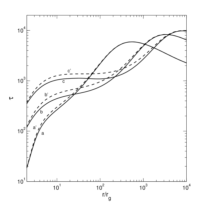
Figure 3: Total optical depth $\tau$ as a function of $r$. Lines $a$, $b$, $c$, $a$’, $b$’, and $c$’ are the correspondents of those in Fig. 1, respectively.

As a check of our global solutions, the total optical depth $\tau=\overline{\kappa}\Sigma/2$ is calculated and is shown in Figure 3, where lines $a$, $b$, $c$, $a$’, $b$’, and $c$’ are the correspondents of lines $a$, $b$, $c$, $a$’, $b$’, and $c$’ in Figures 1 and 2, respectively. It is seen that, similar to the existing slim disk solutions (lines $a$’, $b$’, and $c$’), our global solutions are also optically thick everywhere (lines $a$, $b$, and $c$). But $\tau$ in our solutions is somewhat smaller than that in the existing slim disk solutions, especially in the inner regions. This is because in our solutions, the correctly calculated vertical gravitational force is smaller, then $H$ is larger, $v_{r}$ is larger, and $\Sigma$ is smaller for the same $\dot{M}$; and $\overline{\kappa}$ is almost unchanged, especially in the inner regions where the electron scattering opacity is dominant and is a constant.

3 DISCUSSION

3.1 Waiving hydrostatic equilibrium

Though global solutions with vertical gravitational force correctly calculated can be obtained for $\dot{M}<\dot{M}_{\mathrm{max}}$ as shown in Figures 1, 2, and 3, there seems to be also some inconsistency hidden in these solutions. For high accretion rates, the disk’s relative thickness $H/r$ becomes substantially larger than 1 (lines $b$ and $c$ in Fig. 1); and for the critical value $\dot{M}=31.5\dot{M}_{\mathrm{Edd}}$, $H/r$ reaches up to $\sim 20$ in the middle region of the solution. As argued by Abramowicz et al. (1997), if it is assumed that there is no velocity component in the direction orthogonal to the surface of the disk (i.e., no outflows leaving the disk), then there is a relation $v_{H}/v_{r}=dH/dr$, where $v_{H}$ is the vertical velocity on the surface, and vertical motion should not be neglected if $H$ does not very slowly vary with $r$. In particular, at the maximum of $H/r$ (see lines $b$ and $c$ in Fig. 1), it follows from $d(H/r)/dr=0$ that $dH/dr=H/r$. This means that in the middle region of the solution the vertical velocity could greatly exceed the radial velocity, and the assumption of hydrostatic equilibrium would not be valid. In this case, instead of hydrostatic equilibrium equation (9), one should use the more general form of vertical momentum equation,

$$\frac{1}{\rho}\frac{\partial p}{\partial z}+\frac{\partial\psi}{\partial z}+v_{r}\frac{\partial v_{z}}{\partial r}+v_{z}\frac{\partial v_{z}}{\partial z}=0$$ (20)

(Abramowicz et al. 1997).

Solving this partial differential equation is beyond the capacity of the slim disk model that is one-dimensional. In an illustrative sense, here we wish to try to consider the non-negligible vertical velocity $v_{z}$ with a very simple treatment, which is similar to what was done in Abramowicz et al. (1997). We assume

$$v_{z}(r,z)=\frac{z}{H}v_{H}=\frac{z}{r}u,$$ (21)

where

$$u(r)=v_{r}\frac{d\mathrm{ln}H}{d\mathrm{ln}r},$$ (22)

then equation (20) is reduced to be

$$\frac{1}{\rho}\frac{\partial p}{\partial z}+\frac{\partial\psi}{\partial z}+zY=0,$$ (23)

where

$$Y(r)=\frac{1}{r^{2}}\left(rv_{r}\frac{du}{dr}-v_{r}u+u^{2}\right),$$ (24)

which looks similar to equation (9) of Abramowicz et al. (1997).

Instead of equations (16) and (17), the vertical integration of equation (23) gives (of course, still with the explicit potential eq. [10])

$$g=\left(\frac{\rho}{\rho_{0}}\right)^{1/3}=\left(\frac{p}{p_{0}}\right)^{1/4}=\frac{T}{T_{0}}=\frac{GM(\frac{1}{\sqrt{r^{2}+z^{2}}-r_{g}}-\frac{1}{\sqrt{r^{2}+H^{2}}-r_{g}})+\frac{1}{2}Y(H^{2}-z^{2})}{GM(\frac{1}{r-r_{g}}-\frac{1}{\sqrt{r^{2}+H^{2}}-r_{g}})+\frac{1}{2}YH^{2}},$$ (25)

$$4\frac{p_{0}}{\rho_{0}}=GM\left(\frac{1}{r-r_{g}}-\frac{1}{\sqrt{r^{2}+H^{2}}-r_{g}}\right)+\frac{1}{2}YH^{2}.$$ (26)

Equations (18) and (19) are formally unchanged, but the quantity g in these two equations is given by equation (25) now.

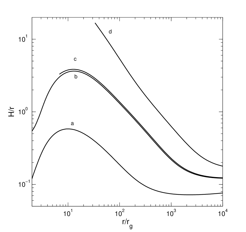
Figure 4: Quantity $H/r$ as a function of $r$ in the case that vertical motion is included. Lines $a$, $b$, $c$, and $d$ are for $\dot{M}/\dot{M}_{\mathrm{Edd}}=$ 1, 8.5, 9, and 30, respectively. There is a new $\dot{M}_{\mathrm{max}}\approx 8.5\dot{M}_{\mathrm{Edd}}$, above which there are no global solutions (lines $c$ and $d$).

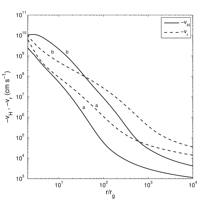
Figure 5: Radial velocity $v_{r}$ and vertical velocity on the disk surface $v_{H}$ in global solutions. Lines $a$ and $b$ are the correspondents of those in Fig. 4, respectively.

The nine equations, i.e., equations (1 - 5), (18), (19), (22), and (26) can be solved for nine unknowns, $\rho_{0}$, $p_{0}$, $\Sigma$, $\Pi$, $T_{0}$, $v_{r}$, $\Omega$, $H$ and $u$ (eq. [1] keeps unchanged even there is a non-zero $v_{z}$, because of the no outflow assumption; and eqs. [2 - 5] still hold as well). The situation of solutions is seen in Figure 4 that shows $H/r$ as a function of $r$. Global solutions exist till a new maximal possible accretion rate $\dot{M}_{\mathrm{max}}\approx 8.5\dot{M}_{\mathrm{Edd}}$ (lines $a$ and $b$ that are for $\dot{m}=1$ and 8.5, respectively), above which there are no global solutions (lines $c$ and $d$ that are for $\dot{m}=9$ and 30, respectively). But this time, for $\dot{M}>\dot{M}_{\mathrm{max}}$, it is not the case of Figure 1 that the inward integration stops at a radius where the thickness $H$ tends to infinity; rather, it is the case that the inward integration stops at a radius where the quantity $g$ of equation (25) tends to become unphysically negative at some height $z$ between the equatorial plane $z=0$ (where $g=1$) and the disk surface $z=H$ (where $g=0$), even though $H$ is finite at that radius. It is not surprising that the value of $\dot{M}_{\mathrm{max}}$ here is even smaller than that in the above section where vertical hydrostatic equilibrium is assumed. The reason for this is the following. As seen from Figure 5, in global solutions $a$ and $b$, $v_{H}$ is always negative, i.e., the vertical motion is always inward towards the equatorial plane; and the absolute value of $v_{H}$ increases with decreasing $r$. This means clearly that there is a vertical acceleration towards the equatorial plane. That is, in the vertical direction, the gravitational force has to overcome the pressure force to accelerate the accreted matter, rather than only balancing the pressure force to ensure hydrostatic equilibrium. The upper limit of the amount of the accreted matter, to which the gravitational force is able to do this harder job, must be smaller than in the hydrostatic equilibrium case. For $\dot{M}>\dot{M}_{\mathrm{max}}$, the gravitational force would be unable to do the job. To keep equation (23) formally holding, $g$ (and $\rho$ and $T$) of equation (25) would have to become mathematically negative, which are physically unacceptable.

Though the treatment of vertical motion made here is crude, it is sayable that inclusion of this motion should not change the main conclusion reached in the above section, i.e., there is a maximal possible accretion rate $\dot{M}_{\mathrm{max}}$ for global slim disk solutions to exist; and the value of $\dot{M}_{\mathrm{max}}$ becomes even smaller than in the case that this motion was omitted.

3.2 Outflows

If the mass accretion rate given at large radii exceeds its maximal possible value, $\dot{M}>\dot{M}_{\mathrm{max}}$, it seems that the only possible way for a global slim disk solution to be realized is that the accretion flow loses its matter at large radii in the form of outflows, such that at smaller radii $\dot{M}$ is reduced to be below $\dot{M}_{\mathrm{max}}$.

Outflows have been observed in many high energy astrophysical systems that are believed to be powered by black hole accretion, but the mechanism of outflow formation remains unclear from the theoretical point of view. At the same time when the ADAF model was proposed, it was suggested that ADAFs are likely to be able to produce outflows because they have a positive Bernoulli constant in their self-similar solutions (Narayan & Yi 1994). Later, Abramowicz et al. (2000) showed that in global solutions of ADAFs the Bernoulli function, rather than the Bernoulli constant, can have either positive or negative values, and that even a positive Bernoulli function is only a necessary, not a sufficient, condition for outflow formation.

Historically, the Bernoulli constant or function was defined as the sum of the specific enthalpy, kinetic energy, and gravitational potential energy. For ADAFs Narayan & Yi (1994) and Abramowicz et al. (2000) discussed, the Bernoulli function has a simple expression since the enthalpy is totally due to the disk gas; it has also a clear physical meaning that its positivity may imply a possibility of outflows. For slim disks, however, the contribution from radiation to the enthalpy becomes important or even dominant over that from gas. To our knowledge, in this case it is unclear whether and how can the Bernoulli function be defined, or whether this function would have the same meaning as for ADAFs if its historical definition is copied. Therefore, we use instead the specific total energy of the matter in slim disks to consider the possibility of outflows, whose equatorial-plane value is

$$E=\left(\frac{3}{2}\frac{k_{\mathrm{B}}T_{0}}{\mu m_{p}}+\frac{aT_{0}^{4}}{\rho_{0}}\right)+\frac{1}{2}\left(v_{r}^{2}+\Omega^{2}r^{2}\right)-\frac{GM}{r-r_{g}}$$ (27)

(cf. eq. [11.33] of Kato et al. 1998).

Figure 6 shows $E$ corresponding to the solutions with the correct gravitational force in Figures 1 and 2. Lines $a$, $b$, $c$, $d$, and $e$ in Figure 6 are for the same physical parameters as lines $a$, $b$, $c$, $d$, and $e$ in Figures 1 and 2, respectively. For accretion rates that allow global solutions to exist, $\dot{M}=1,10$ and $31.5\dot{M}_{\mathrm{Edd}}$ (lines $a$, $b$, and $c$), $E$ is negative everywhere in the disk, and outflows are unlikely to originate. However, for accretion rates exceeding $\dot{M}_{\mathrm{max}}(r)$, $\dot{M}=31.7$ and $100\dot{M}_{\mathrm{Edd}}$ (lines $d$ and $e$), it is seen that as $r$ decreases, $E$ tends to become positive first, and then the solution stops extending. Further, it is noticeable that, when a flow changes from a state represented by line $e$ to a state represented by line $d$, its $E$ increases, and at the same time its $\dot{M}$ decreases. The increase of $E$ favors outflow formation, and the decrease of $\dot{M}$ is just the result of outflows. Such a process of the change of the flow’s state continues until $\dot{M}$ is sufficiently reduced and the flow reaches a state represented by line $c$, then $E$ becomes negative and outflows cease.

To summarize, in this subsection we make two arguments for outflows produced in an accretion flow with large $\dot{M}$ at large radii. First, outflows are necessary because the accretion flow must lose its matter in this way in order to follow a global solution till the central black hole. Second, outflows are possible because the accretion flow can have a positive specific total energy; what is additionally needed for outflows to be realized is that the matter in the accretion flow comes under an outward perturbation in the vertical direction.

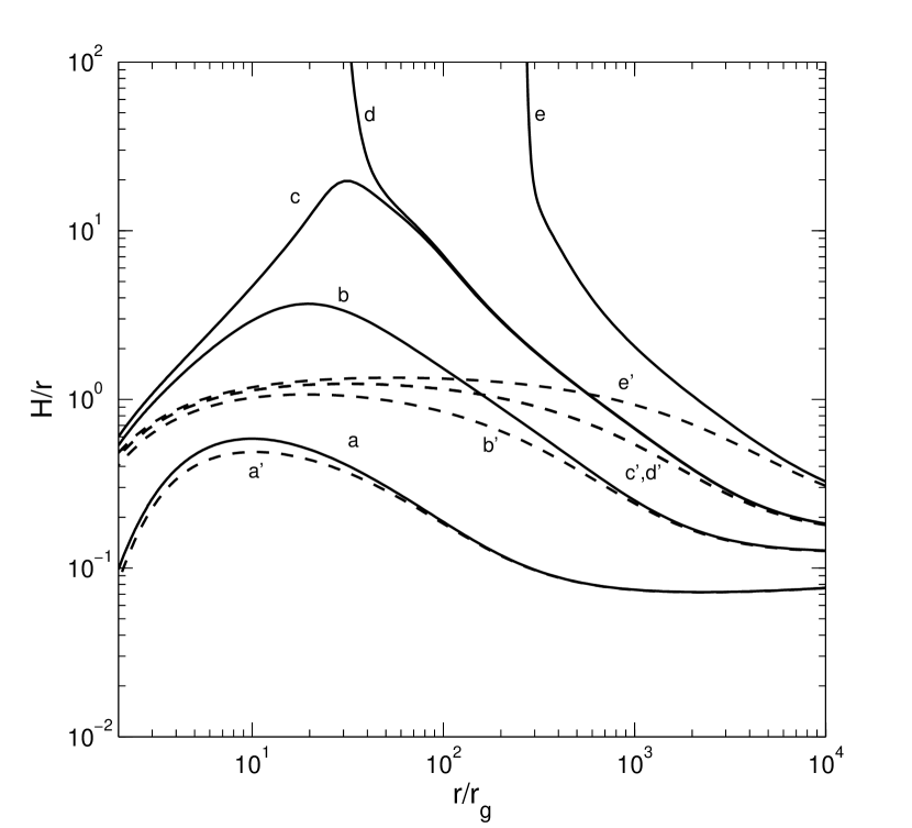
Figure 1: Disk’s relative thickness $H/r$ as a function of $r$. Solid lines represent our results with the vertical gravitational force revised, and dashed lines the results in the existing slim disk model. Lines $a$ and $a$’, $b$ and $b$’, $c$ and $c$’, $d$ and $d$’, and $e$ and $e$’ are for accretion rates $\dot{M}/\dot{M}_{\mathrm{Edd}}=$ 1, 10, 31.5, 31.7, and 100, respectively. There exists a maximal possible accretion rate $\dot{M}_{\mathrm{max}}\approx 31.5\dot{M}_{\mathrm{Edd}}$, above which global solutions cannot be constructed as $H$ tends to infinity (lines $d$ and $e$). Here and in Figs. 2, 3, and 6 the vertical hydrostatic equilibrium is assumed.

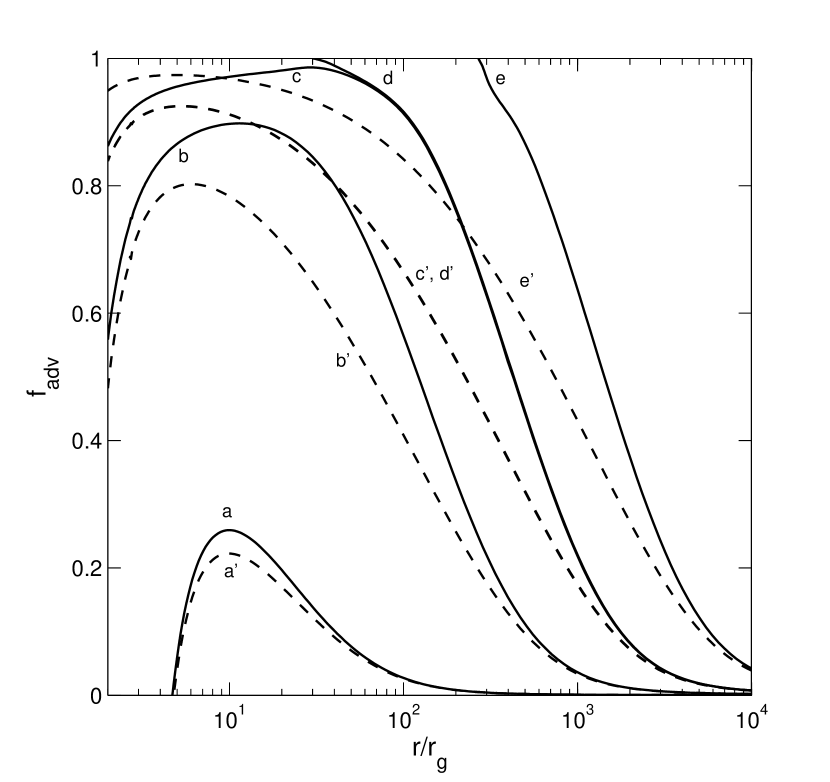
Figure 2: Advective factor $f_{\mathrm{adv}}$ as a function of $r$. All the lines are the correspondents of those in Fig. 1, respectively. Lines $d$ and $e$ are not global solutions as $f_{\mathrm{adv}}$ tends to exceed its maximal possible value 1.

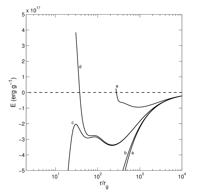
Figure 6: Specific total energy $E$ as a function of $r$. Lines $a$, $b$, $c$, $d$ and $e$ are the correspondents of those in Fig.1, respectively.

References

- (1) Abramowicz, M. A., Chen, X., Kato, S., Lasota, J.-P., & Regev, O. 1995, ApJ, 438, L37
- (2) Abramowicz, M. A., Czerny, B., Lasota, J.-P., & Szuszkiewicz, E. 1988, ApJ, 332, 646
- (3) Abramowicz, M. A., Lanza, A., & Percival, M. J. 1997, ApJ, 479, 179
- (4) Abramowicz, M. A., Lasota, J.-P., & Igumenshchev, I. V. 2000, MNRAS, 314, 775
- (5) Abramowicz, M. A., Lasota, J.-P., & Xu, C. 1986, in IAU Symp. 119, Quasars, ed. G. Swarup & V. K. Kapahi (Dordrecht: Reidel), 371
- (6) Artemova, Y. V., Bisnovatyi-Kpgan, G. S., Igumenshchev, I. V., & Novikov, I. D. 2006, ApJ, 637, 968
- (7) Chen, L.-H., & Wang, J.-M. 2004, ApJ, 614, 101
- (8) Chen, X., Abramowicz, M. A., Lasota, J.-P., Narayan, R., & Yi, I. 1995, ApJ, 443, L61
- (9) Chen, X., & Taam, R. E. 1993, ApJ, 412, 254
- (10) Frank, J., King, A., & Raine, D. 2002, Accretion Power in Astrophysics (Cambridge: Cambridge Univ. Press)
- (11) Gierliński, M., & Done, C. 2004, MNRAS, 347, 885
- (12) Gu, W.-M., & Lu, J.-F. 2007, ApJ, 660, 541 (GL07)
- (13) Gu, W.-M., Xue, L., Liu, T., & Lu, J.-F. 2008, in preparation
- (14) Hōshi, R. 1977, Prog. Theor. Phys., 58, 1191
- (15) Janiuk, A., Czerny, B., & Siemiginowska, A. 2002, ApJ, 576, 908
- (16) Kato, S., Fukue, J., & Mineshige, S. 1998, Black-Hole Accretion Disks (Kyoto: Kyoto Univ. Press)
- (17) Narayan, R., & Yi, I. 1994, ApJ, 428, L13
- (18) Narayan, R., & Yi, I. 1995, ApJ, 444, 231
- (19) Paczyński, B., & Wiita, P. J. 1980, A&A, 88, 23
- (20) Shakura, N. I., & Sunyaev, R. A. 1973, A&A, 24, 337
- (21) Watarai, K. 2006, ApJ, 648, 523
- (22) Watarai, K., Ohsuga, K., Takahashi, R., & Fukue, J. 2005, PASJ, 57, 513