Cataclysmic Variable Primary Effective Temperatures:
Constraints on Binary Angular Momentum Loss

Abstract

We review the most decisive currently available measurements of the surface effective temperatures, $T_{\rm eff}$, of white dwarf (WD) primaries in cataclysmic variables (CVs) during accretion quiescence, and use these as a diagnostic for their time averaged accretion rate, $\langle\dot{M}\rangle$. Using time-dependent calculations of the WD envelope, we investigate the sensitivity of the quiescent $T_{\rm eff}$ to long term variations in the accretion rate. We find that the quiescent $T_{\rm eff}$ provides one of the best available tests of predictions for the angular momentum loss and resultant mass transfer rates which govern the evolution of CVs. While gravitational radiation is completely sufficient to explain the $\langle\dot{M}\rangle$ of strongly magnetic CVs at all $P_{\rm orb}$, faster angular momentum loss is required to explain the temperatures of dwarf nova primaries (non-magnetic systems). This provides evidence that a normal stellar magnetic field structure near the secondary, providing for wind launching and attachment, is essential for the enhanced braking mechanism to work, directly supporting the well-known stellar wind braking hypothesis. The contrast in $\langle\dot{M}\rangle$ is most prominent for orbital periods $P_{\rm orb}>3$ hours, above the so-called period gap, where $\langle\dot{M}\rangle$ differs by orders of magnitude, but a modest enhancement is also present at shorter $P_{\rm orb}$. The averaging time which $\langle\dot{M}\rangle$ reflects depends on $\langle\dot{M}\rangle$ itself, being as much as $10^{5}$ years for low-$\langle\dot{M}\rangle$ systems and as little as $10^{3}$ years for high-$\langle\dot{M}\rangle$ systems. We discuss in some detail the security of conclusions drawn about the CV population in light of these time scales and our necessarily incomplete sample of systems, finding that, due to the time necessary for the quiescent $T_{\rm eff}$ to adjust, the consistency of measurements between different systems places significant constraints on possible long-timescale variation in $\dot{M}$. Measurements for non-magnetic systems above the period gap fall below predictions from traditional stellar wind braking prescriptions, but above more recent predictions with somewhat weaker angular momentum loss. We also discuss the apparently high $T_{\rm eff}$’s found in the VY Scl stars, showing that these most likely indicate $\langle\dot{M}\rangle$ in this subclass even larger than predicted by stellar wind braking.

1. Introduction

The evolution of short-period binaries containing a Roche lobe filling low-mass main sequence (MS) star transferring matter onto a white dwarf (WD), the bulk of the cataclysmic variables (CVs; Warner 1995), has long been believed to be driven by two distinct angular momentum loss mechanisms. Each of these has a distinct rate at which angular momentum is lost, $\dot{J}$, and resulting time-averaged mass transfer rate $\langle\dot{M}\rangle$ required such that the MS star remains within the Roche lobe dimensions. The absolute minimum $\dot{J}$ for the binary is set by losses due to gravitational radiation from the orbital motion itself (Faulkner, 1971; Paczynski & Sienkiewicz, 1981; Rappaport et al., 1982). Higher $\dot{J}$ is obtained due to the partial magnetic attachment of stellar winds similar to those which spin down isolated stars (Verbunt & Zwaan, 1981), which extract angular momentum from the orbit because the Roche lobe filling MS star is tidally locked to the orbit. It was suggested (Paczynski & Sienkiewicz, 1983; Rappaport et al., 1983; Spruit & Ritter, 1983) that the evolution of CVs could be explained by combining these two mechanisms: at long orbital periods, $P_{\rm orb}\gtrsim 3$ hours, when the star has mass $M_{\rm MS}\gtrsim 0.25M_{\odot}$, and can support a typical stellar magnetosphere, wind losses dominate $\dot{J}$, but when $M_{\rm MS}\lesssim 0.25M_{\odot}$, the star’s magnetic structure is disrupted by the loss of the radiative core so that $\dot{J}$ falls to the level of gravitational radiation.

This interrupted magnetic braking (IMB) scenario (see e.g. Hameury et al., 1988; Kolb, 1993; Howell et al., 2001) explains an essential feature of the observed CV population: the lack of systems with $2~{}{\rm hours}\lesssim P_{\rm orb}\lesssim 3$ hours. Systems in this range are predicted to be detached and non-mass transferring because the high mass loss rate to which the MS star was subject during the wind $\dot{J}$ phase is large enough for it to become bloated, such that when $\dot{J}$ decreases and it returns to the equilibrium radius for a main sequence star of the appropriate mass, it is well within the Roche lobe. The orbit must then contract further, to shorter $P_{\rm orb}$, before contact and thus mass transfer is reestablished. Such bloating above the period gap does appear to be borne out by recent studies (Beuermann et al., 1998; Knigge, 2006). While the relation derived from the spindown of cluster stars can, with questionable justification, be extrapolated to the spins appropriate to the CV $P_{\rm orb}$ values, what has actually taken place in practice is that several variations were considered early on (Rappaport et al., 1983) and that which best reproduced the observed period gap was chosen. Thus the mass transfer rate, $\dot{M}$, which IMB predicts above the period gap is that which is necessary to bloat the MS star by the necessary amount to reproduce the $P_{\rm orb}$ extent of the gap itself.

While the IMB scenario of CV evolution does explain the observed period gap, it faces a number of problems. On one hand, observations of single low-mass stars do not show evidence for a change in spin-down rate at the mass boundary where the stars become fully convective (Andronov et al., 2003). On the other hand, most attempts to observationally measure $\dot{M}$ in both $\dot{J}$ regimes have proven difficult. Initial indicators from disk properties (Patterson, 1984) were consistent with the IMB picture, but they lack accuracy as they rely on a number of poorly known system properties, including their distances. Even if successful, $\dot{M}$ determined from accretion disk studies measures only the instantaneous mass transfer rate. Indicators for $\langle\dot{M}\rangle$ from the departure from thermal equilibrium in the donor star appear quite promising, but suffer from the fact that reproducing the radii of isolated stars with these theoretical models is non-trivial (Beuermann, 2006; Ribas, 2006), and the value of $\dot{M}$ derived can be very sensitive to the radius predicted by the model. Townsley & Bildsten (2005) were able to use the period-specific classical nova rate to investigate the $\dot{M}$-$P_{\rm orb}$ relation since the nova ignition mass, and therefore inter-outburst time, depends on $\langle\dot{M}\rangle$. However absolute $\dot{M}$ measurements with this method are elusive due to uncertainties in the mass distribution and CV population density. Measurements of the WD effective temperature, $T_{\rm eff}$, the subject of this paper, provide one of the more promising avenues for constraining the $\dot{M}$ in observed systems. The quiescent $T_{\rm eff}$ expected from a given time average accretion rate $\langle\dot{M}\rangle$ can be calculated directly (Townsley & Bildsten 2003; Townsley & Bildsten 2004; herafter TB03 and TB04), and our discussion will largely be concerned with how representative the $\langle\dot{M}\rangle$ inferred $T_{\rm eff}$ is of the true $\langle\dot{M}\rangle$.

Given that the WDs in CVs are relatively hot objects, $\mbox{$T_{\rm eff}$}\gtrsim 10\,000$ K, their spectral energy distribution peaks in the ultraviolet (UV), and it is in this wavelength range that most of the CVWD $T_{\rm eff}$ measurements were obtained. A handful of bright CVWDs were intensively studies with the International Ultraviolet Explorer (IUE), e.g. VW Hyi (Mateo & Szkody, 1984), WZ Sge (Sion et al., 1990), or AM Her (Heise & Verbunt, 1988; Gänsicke et al., 1995). Temperature estimates obtained prior to the launch Hubble Space Telescope (HST) were summarized by Sion (1991), and updated for measurements obtained predominantly with the HST first-generation UV spectrographs by Sion (1999). A significant increase in the number of reliable CVWD $T_{\rm eff}$ measurements has become available since the deployment of the Space Telescope Imaging Spectrograph (STIS) on HST and the launch of the Far Ultraviolet Spectroscopic Explorer (FUSE), see e.g. Araujo-Betancor et al. (2005b).

We begin by reviewing the relationship between $\langle\dot{M}\rangle$ and $T_{\rm eff}$ as discussed by TB03. The amount of variation expected in $T_{\rm eff}$ due to long term $\dot{M}$ variations is evaluated from both quasi-static models and time-dependent envelope simulations. Following this, in §3, features of the system such as outburst properties, accretion geometry, and possible additional heat sources are discussed to evaluate their impact on the utility of $T_{\rm eff}$ as and indicator of $\langle\dot{M}\rangle$. §4 critically reviews the available measurements of CV WD $T_{\rm eff}$’s, with the intention of selecting a well-understood set of measurements from which firm conclusions on CV properties can be drawn. After some discussion of general uncertainties and biases, §5 sets out our conclusions, including the contrast in $\langle\dot{M}\rangle$ across the gap, the enhanced $\langle\dot{M}\rangle$ in VY Scl-type novalikes displaying low states, and the case for the suppression of wind braking in CVs with highly magnetic WDs.

2. Relationship of $T_{\rm eff}$ to $\dot{M}$

The luminosity streaming up through the surface of the WD during accretion quiescence is released at all depths effectively down to the base of the accreted layer by the compression of material as it is pushed deeper into the star by further accretion (TB04). The infall energy is deposited at very shallow depths and therefore radiates away quickly ($\sim$ hours) after the cessation of active accretion (see §2.3 below for more discussion). Due to the lengthening thermal time with increased depth, a large portion of this quiescent luminosity reflects an accretion history averaged over timescales which can be longer than $10^{4}$ yr, depending on the characteristic value of $\dot{M}$.

As a reference point from which to begin, §2.1 reviews how the quiescent luminosity depends on the time averaged value of the accretion rate, $\langle\dot{M}\rangle$, and other features of the WD. This provides a relation between $T_{\rm eff}$ and $\langle\dot{M}\rangle$ which has no “free” parameters, but does have important but manageable uncertainties related to unknown properties of the WD. Following this, in §2.2 we present a basic discussion of how the response of the envelope to accretion can be understood in terms of the run of local thermal time with depth. This provides justification for the general assertions made above about the timescales on which the surface luminosity can vary. Using estimates of the run of thermal timescale in the outermost portion of the envelope, in §2.3 we derive the timescales on which heat deposited near the surface is radiated away. This demonstrates how measurement of the luminosity escaping due to compression is possible between transient accretion events such as dwarf novae. Such simple estimates are insufficient for characterizing long-term variations, so that we proceed, in §2.4, to discuss and then characterize, with simulations, how long timescale variations in $\dot{M}$ affect the quiescent $T_{\rm eff}$.

2.1. Long Term Average Properties

TB04 presented a detailed discussion of the impact of accretion at rates low enough that hydrogen burns in unstable outbursts, Classical Nova eruptions, on the thermal structure of a WD. For this paper we are primarily interested in the predictions for the quiescent surface luminosity, $L_{\rm q}(M,\langle\dot{M}\rangle,T_{c})$, where $M$ is the WD mass, $\langle\dot{M}\rangle$ is the time-average accretion rate, and $T_{c}$ is the WD core temperature. Through a simple balance of compression of material and radiative heat transport, the quiescent surface luminosity is given by $L_{\rm q}\simeq\langle\dot{M}\rangle T_{b}/\mu m_{p}=4\pi R^{2}\sigma T_{\rm eff}^{4}$ where $T_{b}$ is the temperature at the base of the radiative layers, typically $T_{b}\simeq T_{c}$, $R$ is the WD radius, $\mu$ is the mean molecular weight of the accreted material, $m_{p}$ is the mass of the proton and $\sigma$ is the Stefan-Boltzmann constant. TB04 found that $T_{c}$ approaches an equilibrium value when the WD is subject to accretion at constant $\langle\dot{M}\rangle$ for timescales similar to the WD core thermal time, $\sim 10^{8}$ years. This $T_{c,\rm eq}$ is not strongly sensitive to $M$ and increases weakly with $\langle\dot{M}\rangle$, being generally 0.5 to 1 $\times 10^{7}$ K for CV WDs, which have $\langle\dot{M}\rangle=10^{-11}$ to $10^{-8}M_{\odot}\ {\rm yr^{-1}}$. This equilibrium has recently been demonstrated in simulations which follow the WD evolution through many nova outbursts, finding slightly but not significantly higher $T_{c,\rm eq}$ for the higher $\langle\dot{M}\rangle$’s in this range, and similar evolutionary timescales (Epelstain et al., 2007). $L_{\rm q}$ is insensitive to $T_{c}$ for $T_{c}\leq T_{c,\rm eq}$ and the $\langle\dot{M}\rangle$ relevant above the period gap, where $\langle\dot{M}\rangle$ changes on timescales less than the core thermal time (TB03). Thus we do not need to know the details of $T_{c}$ in order to derive $\langle\dot{M}\rangle$ from $T_{\rm eff}$, though we use $T_{c,\rm eq}$ as a convenient reference value.

Including a small amount of nuclear heating, using the methods of TB04 we find that (at $T_{c,\rm eq}$) the average $L_{\rm q}$ during the classical nova (CN) cycle is

$$L_{\rm q}=6\times 10^{-3}L_{\odot}\left(\frac{\langle\dot{M}\rangle}{10^{-10}M_{\odot}\ {\rm yr^{-1}}}\right)\left(\frac{M}{0.9M_{\odot}}\right)^{0.4}.$$ (1)

Using an approximate power-law relation for $R\propto M^{-1.8}$ near $M=1.0M_{\odot}$, this gives

$$T_{\rm eff}=1.7\times 10^{4}\ {\rm K}\left(\frac{\langle\dot{M}\rangle}{10^{-10}M_{\odot}\ {\rm yr^{-1}}}\right)^{1/4}\left(\frac{M}{0.9M_{\odot}}\right)\ .$$ (2)

As emphasized in TB03, the $\langle\dot{M}\rangle$ inferred from a system’s quiescent $T_{\rm eff}$ is strongly dependent on the assumed $M$, almost entirely due to the use of $R$ to infer $L_{\rm q}$. While $\langle\dot{M}\rangle\propto M^{-3.9}$ for a given $T_{\rm eff}$, $\langle\dot{m}\rangle\equiv\langle\dot{M}\rangle/4\pi R^{2}\propto M^{-0.3}$. Just a 25% uncertainty in mass, allowing $M=0.6$ to $1.0M_{\odot}$, leads to nearly a factor of ten uncertainty in $\langle\dot{M}\rangle$. This seems to be the strongest limit on the utility of measurements of $T_{\rm eff}$, and is difficult to avoid without either independent mass measurements or distances. Only a handful of systems have independent mass measurements (see Table 1), and all but one are DN below the period gap, and the one above is a VY Scl star with a high $\langle\dot{M}\rangle$. It appears infeasible to make conclusions based on a subsample that only includes objects with mass measurements. However, as we will see below, order of magnitude contrasts are easily discernible when the full sample is considered and are important for discriminating between angular momentum loss laws. Additionally, there are now enough sound measurements that further progress can be made with some assumptions about the mass distribution of the population.

The next most important source of uncertainty, which is nearly impossible to eliminate for most systems, is due to the increase in $L_{\rm q}$ as the mass of the accumulated layer, $M_{\rm acc}$, increases between classical nova outbursts. Scatter in the observed $T_{\rm eff}$ values at the level of $\pm 5\%$ is expected due to systems having different $M_{\rm acc}$’s at the current epoch. This degree of scatter is drawn from allowing a range $0.05M_{\rm ign}\leq M_{\rm acc}\leq 0.95M_{\rm ign}$, and, though the full allowed range gives a larger variation, this represents well the size of layer an observed WD is likely have. (See TB04 for details of how $T_{\rm eff}$ varies with $M_{\rm acc}$.) We set the mass fraction $X_{{}^{3}\rm He}=0.001$ in the accreted material throughout this work, because the difference between this and similar predictions for $X_{{}^{3}\rm He}=0.005$ is less than the uncertainty due to the unknown $M_{\rm acc}$ (TB04).

2.2. Envelope Response Timescales

One of the attractions of utilizing $T_{\rm eff}$ as an indicator of $\langle\dot{M}\rangle$ is that $T_{\rm eff}$ contains averaged information about the time history of $\dot{M}$ rather than its instantaneous value. This is of great benefit for comparing $\langle\dot{M}\rangle$ with predictions based on long-term drivers of the binary evolution contributing to orbital angular momentum loss. Before proceeding with simulations of the response of the envelope to $\langle\dot{M}\rangle$ variations, it is useful to first discuss the relevant timescales within the envelope and how they relate to the surface luminosity. We do this in order to understand how much a perturbation on some prescribed timescale is likely to affect the surface luminosity.

The heat equation in the outer layers of the WD is given by (TB04)

$$c_{P}\frac{\partial T}{\partial t}=\frac{\partial F}{\partial y}+c_{P}\dot{m}\frac{T}{y}(\nabla-\nabla_{\rm ad}),$$ (3)

Where $y=\int_{r}^{R}\rho dr\simeq P/g$, the column depth in from the surface ($r=R$), forms a radial coordinate, $P$ is the pressure at radius $r$, $g$ is the surface gravity, $F=(4\sigma T^{3}/3\kappa)dT/dy$ is the local area-specific energy flux with $\sigma$ being the Stefan-Boltzmann constant, $\kappa$ the opacity, $c_{P}$ the specific heat at constant pressure, $\nabla=d\ln T/d\ln P$, $\nabla_{\rm ad}=\partial\ln T/\partial\ln P$ at constant entropy, and $\dot{m}=\dot{M}/4\pi R^{2}$. The temperature profile of the envelope at a given depth, $y$, can change on the thermal time for that layer, which we define by “one-zone” differencing the left hand side and the first right hand term in equation (3), dropping the accretion source term, to obtain,

$$\tau_{\rm th}\equiv\frac{yc_{P}T}{F}\simeq\frac{3\kappa y^{2}c_{P}T}{4\sigma T^{4}}.$$ (4)

In a static envelope state, which is a good approximation for a steady $\dot{M}$ (TB04), $\partial T/\partial t$ is small or zero, so that $\partial F/\partial y$, the contribution to the surface flux from each layer, is set by $\dot{m}$ and local properties of the layer. Thus we expect that variations in $\dot{M}$ will appear as variations in $\partial F/\partial y|_{y}$ after a time $t_{\rm th}(y)$, when that layer can respond. For order unity variations in $\dot{M}$ on a given timescale $t_{\rm var}$, the contribution to $L_{\rm q}$ from layers which have $t_{\rm th}>t_{\rm var}$ will not be affected by the variation, while the contribution from layers with $t_{\rm th}<t_{\rm var}$ will change by unity along with $\dot{M}$. Thus $L({\rm surf})-L(t_{\rm th}=t_{\rm var})$, the contribution to the surface luminosity from the layers outside that with $t_{\rm th}=t_{\rm var}$, evaluated with the average envelope state, provides a reasonable indication of the possible variation in $L_{\rm q}$ which can be expected due to unity-level variations in $\dot{M}$ on a timescale of $t_{\rm var}$. This is very similar to how the characteristic cooling time of a dwarf nova outburst is set by the thermal time at the bottom of the freshly accreted material (Piro et al., 2005).

This analysis no longer applies in the deepest layers where the thermal transport becomes mediated by electron conductivity. This is because the one-zoning used to define $\tau_{\rm th}$ no longer holds. Once $t_{\rm var}$ exceeds the thermal time of the whole radiative layer, we are left with a problem which is more similar to the classic WD cooling problem: an insulating layer which acts as the thermal regulator for the underlying heat reservoir formed by layers which are much more thermally well-coupled by electron conduction. In this case the timescale for further changing $L_{\rm q}$ is expected to approach the CN inter-outburst time, that required to build up the maximum degenerate region.

2.3. Reaching the quiescent $T_{\rm eff}$

With the above estimate for thermal response time with depth, it is useful at this point to discuss specifically the cooling of the thin outer layer that is heated by the infall energy of the accreted matter. This is essential to understanding why the quiescent $T_{\rm eff}$ is a good indicator of the energy being liberated by compression in the deeper layers of the star. When material reaches the surface of a WD via the disk, half of the gravitational infall energy ($GM/R$ per unit mass, where $G$ is Newton’s constant) has been radiated in the disk and the rest is possessed as kinetic energy. This kinetic energy is deposited immediately at the WD surface as the material is stopped and spread by interaction with the surface layers (Piro & Bildsten, 2004). This process can heat the WD surface to quite high temperatures given by $T_{\rm surf}=[(GM\dot{M}/2R)/4\pi R^{2}\sigma]^{1/4}\approx 10^{5}~{}{\rm K}\,(\dot{M}/10^{-8}M_{\odot}~{}{\rm yr}^{-1})^{1/4}(M/0.9M_{\odot})^{1.6}$.

However, this heat does not penetrate the WD due to the opposing thermal gradient in the underlying radiative atmosphere which has a profile characterized by $F_{q}=L_{q}/4\pi R^{2}$ satisfying $4\sigma T^{4}/3\kappa y=F_{q}$. During accretion, the infall heating can penetrate to approximately where the local temperature is the same as $T_{\rm surf}$, or a column depth of $y_{\rm surf}\simeq 4\sigma T_{\rm surf}^{4}/3\kappa F_{\rm q}$. Thus, if $\kappa$ is assumed to be dominated by electron scattering at this depth for simplicity, the mass of the layer heated by infall is $M_{\rm surf}=4\pi R^{2}y_{\rm surf}\simeq 5\times 10^{-11}M_{\odot}(T_{\rm surf}/10^{5}{\,\rm K})^{4}(T_{\rm eff,q}/14\,{\rm kK})^{-4}$. The thermal time for this layer to cool is between $yc_{P}T/F_{\rm surf}$ and $yc_{P}T/F_{\rm q}$ which are $10^{2}$ and $10^{5}$ seconds for $T_{\rm eff,q}=14$ kK. The latter is fairly consistent with the 2.8 days found for the cooling of VW Hyi following a normal outburst (Gänsicke & Beuermann, 1996a). This timescale should be typical for cooling after a normal dwarf nova outburst, but is much shorter than the cooling time after a superoutburst, in which an order of magnitude more material than this is deposited. In that case, in contrast, heat is released on the cooling time for the added material due to its relatively rapid compression (Piro et al., 2005). Note that in reality much of the material added to the WD cools as it spreads over the surface (Piro & Bildsten, 2004) so that the above analysis only applies to the heated region near the equator while the rest of the star remains near $T_{\rm eff,q}$.

2.4. Numerical Simulations of Long Term Accretion Rate Variation

The analysis in §2.2 indicates that a given variation in $\dot{M}$ leads to a larger variation in the quiescent surface flux, $L_{\rm q}$, if it occurs on a longer timescale. That is, the excursion from the average quiescent luminosity $\delta L_{\rm q}=\max|L_{\rm q}-\langle L_{\rm q}\rangle|\approx(L_{\rm q,max}-L_{\rm q,min})/2$ increases with the timescale of $\dot{M}$ variation, $t_{\rm var}$, for a fixed amplitude of $\dot{M}$ variation. Thus very brief variations in $\dot{M}$, such as dwarf novae outbursts, have very little impact on $L_{\rm q}$ despite their large magnitude in $\dot{M}$, once the shallow transient has passed. The luminosity excursion, $\delta L_{\rm q}$, of course also depends on the magnitude of the $\dot{M}$ variation. This dependence is expected to be fairly simple, roughly linear, and therefore we focus here on the dependence on $t_{\rm var}$, which relates to the thermal response time structure of the envelope.

In order to test how $L_{\rm q}$, and therefore the quiescent $T_{\rm eff}$, will vary in response to $\dot{M}$ variations, we have performed simulations of an accreting layer on a WD in the plane-parallel approximation. This approximation is fairly good through the accreted layer and has little impact on the time-variation properties being studied here. A similar approximation, extending only to more shallow depths, was used by Piro et al. (2005) in studying the decline of $T_{\rm eff}$ after a dwarf nova superoutburst. Our numerical treatment is described in the appendix.

As simple experiments, we have applied two forms of long-term $\dot{M}$ variation: sinusoidal, with $\dot{M}=\langle\dot{M}\rangle(1-0.8\sin[\pi t/P_{\rm 1/2}])$, and square wave, with $\dot{M}=\langle\dot{M}\rangle(1-0.8\;\textrm{sign}[\sin(\pi t/P_{\rm 1/2})])$, for a wide range of half-period of $\dot{M}$ variation, $P_{\rm 1/2}$. Short term variations in $\dot{M}$ such as accretion disk cycles (dwarf nova outbursts) are not treated explicitly in order to keep timesteps large.

Figure 1.— Time evolution of quiescent surface flux, $L_{\rm q}=4\pi R^{2}\sigma T_{\rm eff}^{4}$, due to compressional energy release in the envelope for a WD with $M=0.9M_{\odot}$ and $\langle\dot{M}\rangle=5\times 10^{-11}M_{\odot}$ yr^-1. Two variations are applied, a sine (dashed lines) and a square wave (solid lines) both with amplitude of $0.8\langle\dot{M}\rangle$. Two timescales of applied variability are shown, $P_{1/2}=10^{5}$ (left) and $4\times 10^{4}$ yr (right). For the same magnitude variation in $\langle\dot{M}\rangle$, a longer timescale of variation leads to a slightly larger variation in $T_{\rm eff}$.

Figure 1 shows time series of $L_{\rm q}$ and $T_{\rm eff}$ for variations in $\dot{M}$ on two timescales, $P_{1/2}=10^{5}$ and $4\times 10^{4}$ yr. This example uses $M=0.9M_{\odot}$ and $\langle\dot{M}\rangle=5\times 10^{-11}M_{\odot}$ yr^-1, representative of DN systems below the period gap, and has $T_{\rm eff,q}=14$ kK and $M_{\rm ign}=2.3\times 10^{-4}M_{\odot}$. Time zero corresponds to $M_{\rm acc}=0.5M_{\rm ign}$. The model is initialized by starting from the static solution described in TB04 with $M_{\rm acc}=0.25M_{\rm ign}$ and applying $\dot{M}=\langle\dot{M}\rangle$ until $M_{\rm acc}=0.5M_{\rm ign}$ to allow the model to settle on the new numerical grid. In Figure 1, a modest increase in the total variation is observed with the square wave $\dot{M}$ applied instead of the sinusoid. There is no appreciable phase difference between the applied $\dot{M}$ variation and that the response. As expected, for the same $\langle\dot{M}\rangle$ and magnitude of $\langle\dot{M}\rangle$ variation, a longer timescale leads to a larger variation in $T_{\rm eff}$. Consecutive peaks are slightly increasing due to the increasing $M_{\rm acc}$ during the buildup to classical nova, the longer displayed example making it to nearly $M_{\rm acc}=0.59M_{\rm ign}$.

Figure 2.— Fractional excursion in quiescent surface flux, $\delta L_{\rm q}/\langle L_{\rm q}\rangle=(L_{\rm q,max}-L_{\rm q,min})/2\langle L_{\rm q}\rangle$, as a function of timescale of the applied $\dot{M}$ variability, $t_{\rm var}$. The response of an envelope simulation to a $0.8\langle\dot{M}\rangle$ variation in $\dot{M}$ is shown for a square (solid) and sinusoidal (dashed) variation. One mass is shown for $\langle\dot{M}\rangle=2\times 10^{-9}M_{\odot}$ yr^-1, with $M=0.9M_{\odot}$, (far upper) and two for $\langle\dot{M}\rangle=5\times 10^{-11}M_{\odot}$ yr^-1, with $M=0.9$ (middle) and $0.6M_{\odot}$ (lower). These cases have $\langle L_{\rm q}\rangle$ ($\langle T_{\rm eff}\rangle$) of 120, 2.8, and 2.6 $\times 10^{-3}L_{\odot}$ (35, 14, and 12 kK) respectively. Also shown for comparison (dot-dash lines) is the run of $[L({\rm surf})-L(t_{\rm th}=t_{\rm var})]/\langle L_{\rm q}\rangle$ in a static approximation of the average envelope state. This represents at what depth, in terms of timescale, energy is being released by compression, and provides a good estimate of the variation expected in response to order unity $\dot{M}$ variation except at the deepest parts of the envelope where electron conduction becomes important.

There is a tremendous contrast between observable timescales of tens of years, and the time between classical nova outbursts which can be as much as $10^{8}$ years depending on $\langle\dot{M}\rangle$. In order to probe this variety, we have performed the same 5-cycle simulations shown in Figure 1 for variability timescales up to about 2.5% of the classical nova accumulation time, making the total simulation time about 25% of the accumulation time. We characterize the variation in $L_{\rm q}$ by its excursion $\delta L_{\rm q}\approx\langle L_{\rm q,max}-L_{\rm q,min}\rangle/2$, where the maximum and minimum are evaluated for each cycle and the difference is then averaged over all cycles. This is then divided by the mean, $\langle L_{\rm q}\rangle$, to obtain a fractional variation. Figure 2 shows the excursion found from the numerical simulations using square (solid lines) and sine (dashed lines) wave $\dot{M}$. Three cases are shown, $M=0.9M_{\odot}$ with $\langle\dot{M}\rangle=2\times 10^{-9}M_{\odot}$ yr^-1 and $M=0.9$ and $0.6M_{\odot}$ with $\langle\dot{M}\rangle=5\times 10^{-11}M_{\odot}$ yr^-1. These have $\langle L_{\rm q}\rangle$ ($T_{\rm eff}$) of 120, 2.8, and 2.6 $\times 10^{-3}L_{\odot}$ (35, 14, and 12 kK) respectively, $M_{\rm ign}$ of 2.2, 23 and 39$\times 10^{-5}M_{\odot}$, time between classical novae of $1.1\times 10^{4}$, $4.6\times 10^{6}$ and $7.8\times 10^{6}$ yr, and $T_{c}$ of 9.6, 5.7 and $5.7\times 10^{6}$ K.

As discussed in §2.2, the magnitude of the variation or excursion in $L_{\rm q}$ can be estimated by evaluating the compressional heat release at depths with thermal time less than $t_{\rm var}$. This can be expressed as $L({\rm surf})-L(t_{\rm th}=t_{\rm var})$, where the quiescent surface luminosity, $L(\rm surf)$ and the luminosity at the depth where the thermal time matches the variation time of the applied $\dot{M}$ variation, $L(t_{\rm th}=t_{\rm var})$ are evaluated from the run of $L$ and $t_{\rm th}$ in a static accreting envelope at $\dot{M}=\langle\dot{M}\rangle$, $L(\rm surf)=\langle L_{\rm q}\rangle$ and $M_{\rm acc}=0.5M_{\rm ign}$. These curves are shown for comparison in Figure 2, one for each case shown from the time-dependent simulations.

We find that $L({\rm surf})-L(t_{\rm th}=t_{\rm var})$ provides a good estimate of the variability until electron conduction becomes important, $t_{\rm th}\gtrsim 10^{4}$ yr. Deeper than this, the $t_{\rm th}$ we have defined underestimates the thermal time, so that $L(t_{\rm th}=t_{\rm var})$ is being evaluated at too deep a layer and $L({\rm surf})-L(t_{\rm th}=t_{\rm var})$ is therefore being overestimated. The variability seen in $L_{\rm q}$ in the simulations does not increase for longer timescales, due to the increased heat capacity from the thermally connected layers where electron conduction provides heat transport that is efficient relative to the overlying radiative layer. We find that the averaging time for a given system depends strongly on its $\langle\dot{M}\rangle$. This is due to the fact that while the luminosity varies by two orders of magnitude (approximately $\propto\langle\dot{M}\rangle$) for CVs, the thermal content of the radiative layers of the envelope changes little with $\langle\dot{M}\rangle$. Note that we have only explored order unity $\dot{M}$ variations here for simplicity of demonstration, smaller variations will lead to correspondingly smaller responses.

The magnitude of the variation in quiescent surface luminosity, $L_{\rm q}$, depends on the timescale of the proposed variation in $\dot{M}$. Since the the $\langle\dot{M}\rangle$ inferred from $T_{\rm eff}$ is approximately proportional to the corresponding $L_{\rm q}$, fractional variations induced in $L_{\rm q}$ by a time-variable $\dot{M}$ correspond directly to fractional uncertainty in an inferred $\langle\dot{M}\rangle$. Since Figure 2 shows the response to an order-unity variation in $\dot{M}$, it also approximately quantifies the fractional uncertainty for a given timescale of variation. Assuming that $\dot{M}$ has only short or moderate timescale variations, even up to $10^{3}$ yr, but is consistent on longer timescales, $T_{\rm eff}$ is a good indicator of the time-averaged $\dot{M}$, with minimal uncertainty (20%) at low $\dot{M}$ and moderate (50%) at high $\dot{M}$. However, due to the long but finite thermal time of the envelope, under the assumption that $\dot{M}$ varies over very long timescales ($>10^{3}$ yr for high-$\dot{M}$ systems or $>10^{5}$ yr for low-$\dot{M}$ systems), $T_{\rm eff}$ is not a reliable indicator of $\langle\dot{M}\rangle$, having a large uncertainty. In this case $T_{\rm eff}$ depends more strongly on the recent accretion history than the overall average. Thus the character of the mass-transfer law being tested must be considered when $T_{\rm eff}$ measurements are used to infer $\langle\dot{M}\rangle$ values. The utility of this relationship between uncertainty and timescale and its application to candidate mass-transfer scenarios is discussed in more detail in §5. There, multiple $T_{\rm eff}$ measurements from similar systems are used to obtain an independent constraint on the time-variability of $\dot{M}$, removing the a priori model dependence for some systems.

3. System Features Affecting the Utility of $T_{\rm eff}$

In addition to long-timescale variations in the mass transfer rate, several features of the systems in which the quiescent $T_{\rm eff}$ measurements can be made affect our ability to determine $L_{\rm q}$ from observations. While we believe that these issues can be avoided by careful selection and interpretation of observations, it is worth summarizing the relevant issues to justify this assertion. Piro et al. (2005) have performed an excellent analysis of how a dwarf nova cools after outburst, finding that the cooling time depends on the amount of matter accreted in the outburst. We therefore forego a detailed discussion of those systems, only noting that care is typically taken that $T_{\rm eff}$ is measured as far in quiescence as is feasible. The other important kinds of systems in which $T_{\rm eff}$ can be measured appropriately are novalike variables during extended quiescence intervals and Magnetic CVs, again in quiescence, where material impacts on a small portion of the WD surface, and the emission from the rest of the star, reflecting $L_{\rm q}$, can be separated. After discussing these two cases we provide a direct estimate of the timescale on which a CVWD would cool to $T_{\rm eff,q}$ after a thermonuclear runaway, and close with a brief discussion of additional energy sources related to accretion which could cause the $T_{\rm eff}$ observed to differ from our calculated $L_{\rm q}$.

3.1. Cooling From High State

In the VY Scl stars discussed in section 4.2, the high $\dot{M}\sim 10^{-8}M_{\odot}$ yr^-1 will, on rare occasions, turn off for timescales of up to a few years. This provides a window in which to measure the $T_{\rm eff}$. As discussed above in section 2.2, the layer which is heated by infall cools in $\sim$100 seconds at this high $\dot{M}$ and resulting high $T_{\rm eff,q}$. Since the outer layers, which can change their thermal state during quiescence, contribute a relatively small fraction of the overall $L_{\rm q}$, the cooling during the quiescence is modest. In Figure 3 we have calculated an example evolution for the $\sim$3-year quiescence of TT Ari during which it was observed twice (Gänsicke et al., 1999), assuming various high state durations between regularly repeated quiescent intervals. With this type of analysis we are able to solve directly for the actual $\langle\dot{M}\rangle=4.1\pm 0.8\times 10^{-9}M_{\odot}$ yr^-1 for $M=0.9M_{\odot}$, accounting for the cooling of the outer layers during quiescence. It is observed from Figure 3 that the $T_{\rm eff}$ flattens out as the thermal time of the cooling layer becomes longer, in such a way that the two epochs of measurements (shown) will be the same within the observational error. By varying the high state interval at fixed $\langle\dot{M}\rangle$, we see that, even for durations as short as 10 years, the quiescent flux is a good indicator of $\langle\dot{M}\rangle$ instead of the high-state $\dot{M}$. The $L_{\rm q}$ scales linearly with $\langle\dot{M}\rangle$ as expected.

Figure 3.— Decline of $T_{\rm eff}$ for the 3-year low state of the novalike TT Ari during 1982-4. UV spectral observations taken at approximately 1 and 2 years after the decline into the low state are both consistent with $T_{\rm eff}=39000\pm 2000$ K (Gänsicke et al., 1999). The three example cases shown have the same $\langle\dot{M}\rangle=4.1\times 10^{-9}M_{\odot}$ yr^-1 but different high state durations: 30 yr (solid), 10 yr (dashed), and 90 yr (dot-dashed).

3.2. Polar Accretion

The geometry of the accretion on the WD surface differs significantly for a strongly magnetic WD ($B\sim 10^{7}$-$10^{8}$ G), in which case mass is deposited at the magnetic poles. However, due to the depth at which this material must spread over the star and the depths at which energy is liberated by compression, the effect on the $T_{\rm eff}$ measured away from the polar regions is modest. The magnetic field can only constrain the accreted material to the polar regions down to a limited pressure depth, $P_{\rm crit}$, below which lateral pressure gradients are strong enough to force the material to spread over the surface. Heat liberated by compression up to $P_{\rm crit}$ is localized to the polar regions, while that from compression at higher pressures is spread over the whole surface.

The magnetic field can keep the accreted material constrained to the WD poles up to a depth where $\beta_{\rm crit}\simeq 2\ell/h$ (Hameury et al., 1983) where $\beta=P/4\pi B^{2}$ is the ratio of gas to magnetic field pressure, $\ell$ is the size of the polar cap, and $h$ is its thickness. Using $h=P/\rho g$, $\ell=10^{8}$ cm and a degenerate equation of state we find that $P_{\rm crit}\sim 10^{15}\ {\rm erg}\ {\rm cm^{-3}}\ (g_{8}\ell_{8}B_{7}^{2})^{5/7}$, where a subscript $s$ indicate values divided by $10^{s}$ cgs units, e.g. $g_{8}=g/10^{8}\ {\rm cm}\ {\rm s^{2}}$. Note that a nondegenerate calculation, which is more appropriate since degeneracy sets in at $P\simeq 10^{17}$ erg cm^-3 for $T_{c}=10^{7}$ K, would give even lower $P_{\rm crit}$. We forgo such a calculation here since the difference does not impact our conclusions.

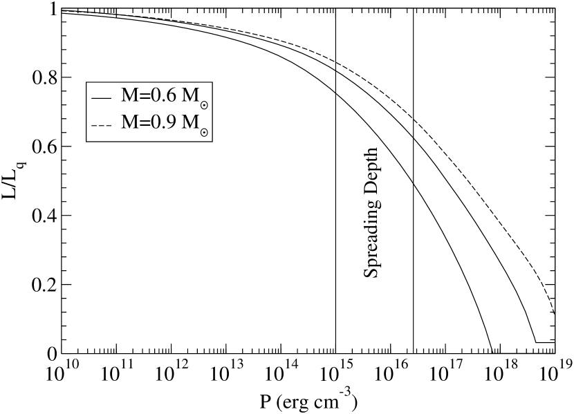
Figure 4.— Luminosity as a function of depth as measured by $P$ as a fraction of $L_{\rm surf}$. The three cases shown are for $\langle\dot{M}\rangle=2\times 10^{-9}$ (lower) and $5\times 10^{-11}M_{\odot}$ yr^-1 (upper) at $M=0.6M_{\odot}$ (solid) and only the lower $\langle\dot{M}\rangle$ at $M=0.9M_{\odot}$ (dashed). These have $L_{\rm q}$ ($T_{\rm eff}$) of 140, 2.6 and 2.8 $\times 10^{-3}L_{\odot}$ (32, 12, and 14 kK). The bulk of the compressional luminosity is released below the depth at which spreading occurs.

As discussed above, energy is liberated by compression at all depths, with much coming from deep in the accreted layer. Figure 4 shows how $L/L_{\rm q}$ varies with depth into the star as measured by $P$. In a magnetic CV WD, we assume that accreted matter spreads over the WD surface at approximately $P_{\rm crit}$, so that only $L|_{P=P_{\rm crit}}$ is released over the whole surface of the star. For typical fields of $10^{7}$ G, this amounts to better than 80% of the $L_{\rm q}$ expected in the non-magnetic case. Thus magnetic CV $T_{\rm eff}$’s warrant a small upward correction from the simple relation given by eq. (2) to obtain the actual $\langle\dot{M}\rangle$.

3.3. Cooling After Thermonuclear Runaway

After shutoff of the nuclear burning in a classical nova, due to heat leftover from the outburst it will take some period of time for $T_{\rm eff}$ to return to that characteristic of $\langle\dot{M}\rangle$. Although this timescale could vary widely depending on how much of the burning envelope is actually left behind on the WD, it appears that in most cases the ejected matter is similar to or larger than the total accreted, indicating that this layer is fairly thin (TB04). The enhancement of the temperature below the burning layer is expected to be modest, being limited to just above $10^{7}$ K by the onset of the instability. A useful estimate for the cooling time is then to take the cooling time of the outer radiative layer. Using $L_{\rm q}$, the endpoint luminosity of the decline, to estimate this cooling time gives a good upper limit on the decline from the hot outburst state.

The mass coordinate, measured in from the surface, where the free-free opacity and that due to conduction are equal is $\Delta M\simeq 4\times 10^{-6}M_{\odot}(M/0.9M_{\odot})^{-8.2}$ for an interior temperature of $10^{7}$ K. This leads to a thermal time of the radiative layer of

$$\tau_{\rm th,rad}\simeq 7\times 10^{4}{\rm\ yr}\left(\frac{T_{\rm eff}}{14{\rm kK}}\right)^{-4}\left(\frac{M}{0.9M_{\odot}}\right)^{-4.6}\ ,$$ (5)

where we have used the approximate dependence $R\propto M^{-1.8}$. Note that this is similar to the timescale at which the response curves from above the variation analysis (see Figure 2) flatten off. This is reasonably consistent with the timescale found by Prialnik (1986) from nova simulations at high mass, $M=1.25M_{\odot}$. This is generally much shorter than the inter-outburst time and therefore we expect few objects to show such an enhancement. If the heated region extends deep enough for some degenerate material to have a longer cooling time, which may be the case at low $\langle\dot{M}\rangle$, it would introduce an enhanced lower boundary temperature for the fresh envelope for a longer time. However, this will not lead to significant enhancement of $L_{\rm q}$ because $L_{\rm q}$ is much larger than the cooling luminosity set only by the modestly increased temperature at the base of the layer.

3.4. Possible Additional Heat Sources

If there is a heat source depositing excess energy at the WD surface during quiescence, this can lead to misinterpretation of the quiescent $T_{\rm eff}$ as representative of $L_{\rm q}$. The energy release due to infall is much larger than that due to compression in the WD, so that a small amount of steady accretion during quiescence in non-magnetic systems could compete with the flux from below in heating the WD surface. Most of the energy from quiescent accretion is expected to appear in the X-rays and typical X-ray luminosities from dwarf novae are $10^{30}-10^{31}$ erg s^-1 (Verbunt et al., 1997) requiring a quiescent $\dot{M}\sim 10^{-12}M_{\odot}$ yr^-1. While this is clearly less than the luminosity of the brighter systems we will consider, it is only slightly less than the lowest $L_{\rm q}\sim 10^{31}$ erg s^-1 ($T_{\rm eff}=14$ kK, $M=0.9M_{\odot}$) that we are considering here. We will ignore this contribution in the first approximation for two reasons. First, it is not expected that $L_{\rm UV}$ and $L_{\rm X}$ should be similar, if anything $L_{\rm UV}$ should be much lower, if there is a steady state corona above the WD surface where the infall energy is released. Any heating which modifies $T_{\rm eff}$ must be deposited at the photosphere, and no higher. Second, while there is a wide variety of X-ray luminosities for dim DN which has no clear cause, we will show that the $T_{\rm eff}$ for these systems show relatively little scatter. At worst our dimmest systems provide upper limits on the $\langle\dot{M}\rangle$ if some portion of the flux is attributed to accretion in quiescence.

4. Measurements of CV Primary $T_{\rm eff}$

The most commonly used method to determine WD effective temperatures in CVs is to fit synthetic spectra to optical and/or ultraviolet (UV) observations. While for single white dwarfs accurate temperatures and good estimates of the surface gravity (and hence, adopting a mass-radius relationship, the WD mass) are routinely derived from spectral fits to the Balmer lines alone, a number of caveats have to be considered when applying such spectral fits to the observations of CVWDs. One main disadvantage encountered in CVs is that their optical light is a mixture of emission from the accretion disk or stream, hot spots on the disk edge or WD surface, from the donor star, and finally from the accreting WD. In the majority of CVs, the WD contributes only a small fraction to the emission at optical wavelengths, which foibles any attempt to determine its properties from ground-based observations. Even in the cases where the WD is a significant source of optical flux, implying low prevailing accretion rates, temperature measurements are subject to a major ambiguity: the strength of the Balmer lines reaches a maximum around 15 000 K, with the exact value being a function of surface gravity, and nearly equally good fits can be achieved on the ”hot” and the ”cold” side.

Because the WDs in CVs are moderately hot, $10\,000-50\,000$ K, their spectral energy distribution peaks in the UV, and therefore the most reliable information on CVWDs is obtained from space-based telescopes such as the IUE, HST, or FUSE. Besides a larger, or dominant, WD contribution to the total UV flux from the CV compared to the optical, the degeneracy between hot and cold Balmer line fits is broken by the opacity of quasimolecular H${}_{2}^{+}$ and H₂, which causes broad absorption lines near 1400 Å and 1600 Å for temperatures below $\sim 18\,000$ K and $\sim 13\,000$ K, respectively (Koester et al., 1985). Examples of the degree of uncertainty in temperatures based on optical data are GW Lib and LL And, where Szkody et al. (2000b) and Szkody et al. (2000a) estimated $\mbox{$T_{\rm eff}$}\simeq 11\,000$ K from optical data obtained during quiescence, whereas the temperatures determined from HST/STIS spectroscopy are $14\,000-15\,000$ K (Szkody et al., 2002a; Howell et al., 2002). While UV spectroscopy can provide fairly accurate WD effective temperatures, its diagnostic potential for determining the surface gravity, $\log g$, is very limited, and so is, therefore, the ability to derive the white dwarf mass from spectral fits.

A remaining issue in modelling the UV data of accreting white dwarfs is that a large fraction display a second continuum flux component, that typically contributes $10-30$%. A number of suggestions for the nature of this component have been made, such as optically thick hot accretion belts on the WD (e.g. Long et al. 1993; Gänsicke & Beuermann 1996b; Huang et al. 1996), optically thick emission from the hot spot or optically thin emission from a chromosphere on the accretion disk (e.g. Gänsicke et al. 2005). While the exact nature of this additional component is not clear, and may well differ among the objects, its impact on the effective temperature determination appears to be only modest.

An alternative method that yields WD effective temperatures, as well as potentially radii and masses as well, is the modelling of the WD ingress/egress in multi-color light curves of eclipsing CVs (Wood & Horne, 1990). The application of that method has been limited until recently to a handful of bright CVs, but since the fast triple-beam CCD camera ULTRACAM (Dhillon et al., 2007) became available on 4 m and 8 m telescopes, a number of detailed CVWD studies have been carried out (e.g. Littlefair et al. 2006b).

The literature is humming with values of CVWD temperatures and some care has to be taken to differentiate between measurements and estimates. For some purposes, it may be desirable to maximize the number of available $T_{\rm eff}$ values, such as provided e.g. by Winter & Sion (2003) and Urban & Sion (2006). In the context of providing a stringent test of the theory angular momentum loss in CVs, we focus here on the most accurate $T_{\rm eff}$ measurements. Table 1 lists CVWD $T_{\rm eff}$ values that we consider reliable on the basis that the WD has unambiguously been detected either spectroscopically, or, in the case of eclipsing systems, through its eclipse ingress/egress. Below in Sect. 4.1–4.3, we discuss particular issues that relate to the effective temperature measurements in the three major CV subclasses, and summarize in Sect. 4.4

4.1. Dwarf novae

Dwarf novae are a subset of non-magnetic CVs with low mass transfer rates. The accretion disks in these systems are thermally unstable, and undergo outbursts lasting a few days to a few months with recurrence times of a few weeks to tens of years. Despite their relatively low mass transfer rates, only a relatively small number of dwarf novae reveal their accreting white dwarfs at optical wavelengths, e.g. WZ Sge (Greenstein, 1957) or VW Hyi (Mateo & Szkody, 1984; Smith et al., 2006). Moving to the UV, about a third of all short-period dwarf novae are dominated by emission from the white dwarf. It is currently unclear why dwarf novae with nearly identical orbital periods and outburst frequencies differ radically in the characteristics of their UV spectra, such as e.g. VW Hyi and WX Hyi, with the first one being one of the best-studied CVWDs (Mateo & Szkody, 1984; Sion et al., 1995b; Gänsicke & Beuermann, 1996a; Long et al., 1996; Smith et al., 2006) and WX Hyi, where no convincing spectroscopic signature from the WD has been detected (Long et al., 2005). The fraction of dwarf novae above the period gap where the WD is clearly discernible in the UV is much smaller than at short orbital periods, as the accretion disks in these systems are larger and can sustain higher accretion rates while still remaining in quiescence.

During dwarf nova outbursts, the accretion rate onto the white dwarf increases by several orders of magnitude with respect to the quiescent value, causing a short-term heating effect (Sion, 1995; Gänsicke & Beuermann, 1996b; Cheng et al., 2000; Godon et al., 2004; Piro et al., 2005). Therefore, when determining the secular WD effective temperature, care has to be taken to observe dwarf novae as long as possible after an outburst. In systems with very short outburst recurrence times, it may be that the WD never cools to its secular temperature (Gänsicke & Beuermann, 1996b). (See also the discussion in §2.3.)

A final caveat relates to the spectral modelling of high-inclination dwarf novae, where the line-of-sight passes through absorbing material located above the accretion disk, termed an accretion veil, affecting the effective temperature determination. In the case of OY Car, a fit ignoring the veiling component yields $T_{\mathrm{eff}}\approx 15\,000$ K (Horne et al., 1994), whereas $T_{\mathrm{eff}}\approx 17\,000$ K when taking the absorption into account (Horne et al., 1994; Cheng et al., 2000). While the effect is noticeable at inclinations $\gtrsim 70^{\circ}$ (e.g. Long et al. (2006), it is most problematic at higher inclinations where the WD eclipse offers an alternative/independent possibility of a $T_{\mathrm{eff}}$ measurement (e.g. Littlefair et al. 2006a).

4.2. Novalikes and the case of VY Scl stars

Novalike variables are non-magnetic CVs, mainly with periods $>3$ h, with high mass transfer rates in which the accretion disk is in a stable hot and optically thick state. Consequently, the flux of novalike variables is entirely dominated by the disk at optical and ultraviolet wavelengths. The only possibility to learn about the properties of WDs in novalike variables occurs if the mass transfer decreases, or turns off completely, so that the WD becomes visible. Novalike variables who show such low states are called VY Scl stars, after the prototypical system, and are found predominantly in the orbital period range $3-4$ h. The physical cause of the occurrence of low states is not fully understood, and may be related to star spots on the secondary star (Livio & Pringle, 1994; Hessman et al., 2000) or irradiation driven mass transfer cycles (Wu et al., 1995).

Due to the rare and unpredictable nature of low states, only three novalike variables have been studied at a sufficient level of detail: TT Ari (Shafter et al., 1985; Gänsicke et al., 1999), DW UMa (Knigge et al., 2000; Araujo-Betancor et al., 2003) and MV Lyr (Hoard et al., 2004). In all three systems, hot $T_{\mathrm{wd}}\gtrsim 40\,000$ K are found.

4.3. Polars

Polars, or AM Herculis stars, contain strongly magnetic WDs. The rotation of the white dwarf is synchronized with the orbital period, and the formation of an accretion disk is suppressed. Accretion occurs via an accretion stream that feeds matter onto the magnetic pole of the WD. Polars enter low states with little or no accretion, and during these episodes the systems appear practically as a detached WD plus main sequence star. However, while the white dwarf is fully exposed during low states, its magnetic field complicates accurate $T_{\mathrm{eff}}$ determinations, as the Balmer lines are subject to Zeeman splitting, and no accurate theory for the line profiles of the Zeeman components exists so far (Jordan, 1992). Zeeman splitting is much weaker for the Lyman lines, and for fields $\lesssim 30$ MG the effect of the magnetic field on temperatures obtained from UV observations around Ly$\alpha$ is relatively small. The polars in Table 1 have all fields $\lesssim 30$ MG at the primary accretion pole, with the exception of QS Tel and V1043 Cen (both $B\simeq 56$ MG).

For stronger fields, even the Lyman lines become useless for temperature estimates, and, worse, the spectral models fail to even reproduce the UV/optical spectral energy distribution, an effect known from single white dwarfs (Schmidt et al., 1986). Consequently, the WD temperatures of high field polars are only very approximatively known, $15\,000-25\,000$ K for AR UMa (Gänsicke et al., 2001) and $17\,000-23\,000$ K for RX J1554.2+2721 (Gänsicke et al., 2004b).

The highly asymmetric accretion geometry in polars results in heating part of the WD atmosphere around the magnetic pole(s) (Gänsicke et al., 1995). As the magnetic axis of the WD is usually not aligned with its spin axis, the heated pole cap acts as a light house, causing a significant variation of the UV flux as a function of WD spin/orbital phase. The pole caps are observed also during low states, and it is not clear if this is due to deep heating, or to residual low-level accretion in the low state (Stockman et al., 1994; Gänsicke et al., 1995). In some polars, the geometry is favorable and the heated pole cap is eclipsed by the body of the white dwarf for part of the orbital cycle, allowing an accurate determination of $T_{\mathrm{eff}}$ from phase-resolved spectroscopy (Gänsicke et al., 2006). If the pole cap contributes at all phases to the UV light, or only phase-averaged data is available, the data can be fit with a two-component model (e.g. Gänsicke et al., 2000; Araujo-Betancor et al., 2005b). $T_{\mathrm{eff}}$ from such analyses provides an upper limit to the true WD temperature.

4.4. Reliable $T_{\rm eff}$ measurements

In the context of using $T_{\rm eff}$ as a measurable quantity that allows insight into the secular averages of the mass transfer rates in CVs, we have included in Table 1 only those systems which we feel have a reliable $T_{\rm eff}$ determination. Consequently, we omitted systems with published WD temperatures where the evidence for seeing the WD is ambiguous. Examples of such cases are WX Hyi, SS Cyg, and RU Peg (Sion & Urban, 2002; Long et al., 2005), where a plausible WD model fit to the UV spectra can be achieved, but no clear WD features are discerned (broad Lyman lines, narrow metal absorption lines). The decision of admitting a system to Table 1 is necessarily subject to a gray area, where some spectroscopic evidence for the WD is present, but not sufficient for an accurate $T_{\mathrm{eff}}$ determination, such as e.g. the case of Z Cam (Hartley et al., 2005). Gänsicke & Koester (1999) have shown that in the case of low spectral resolution and low signal-to-noise the UV data may be equally well described by a moderately hot WD or by an optically thick accretion disk. In this particular case, AH Men, the WD case can be excluded on the basis of the optical properties of the star, providing a clear warning against interpreting a slight flux turnover below 1300 Å as broad L$\alpha$ from a WD photosphere.

In the case of eclipse light curve analyses, we excluded a number of systems where we considered the data of too low quality, i.e. an at best marginal detection of the WD ingress/egress, as well as studies using oversimplified models, such as approximating the WD emission in the different observed wave bands by blackbody radiation.

In recent years, a number of strongly magnetic close WD+MS binaries were identified that contain very cool ($\mbox{$T_{\rm eff}$}\lesssim 9000$ K) WDs and have mass transfer rates, as determined from X-ray observations, of a few $10^{-13}\dot{M}\,\mathrm{yr^{-1}}$ (e.g. Reimers & Hagen, 2000; Szkody et al., 2003a; Schmidt et al., 2005; Vogel et al., 2007). Given the fact that many of them have MS companions that have spectral types too late to be Roche-lobe filling at the orbital periods of the binaries, Webbink & Wickramasinghe (2005) suggested that these systems are pre-CVs that have not yet evolved into a semi-detached configuration. The low mass transfer rates are compatible with wind accretion, and the low WD temperatures match with the predictions for the average life time of pre-CVs Schreiber & Gänsicke (2003). Consequently, we exclude those systems from the present discussion.

A final note concerns the intermediate polars (IPs), a class of weakly magnetic CVs in which the WD spin period is shorter than the orbital period, and partial accretion disks may form. In most IPs, the accretion rate is too high to discern the WD even at UV wavelengths (e.g. Mouchet et al., 1991; Beuermann et al., 2004). In a few IPs, moderately broad Balmer absorption lines were detected in the optical (e.g. Haberl et al., 2002) but a more detailed analysis of the system parameters, in particular the distance, ruled out a WD photospheric origin of these features (de Martino et al., 2006) In the case of EX Hya (Eisenbart et al., 2002; Belle et al., 2003) and AE Aqr (Eracleous et al., 1994) HST spectroscopy provided more convincing evidence for the detection of thermal emission from the WD photosphere, compatible with temperatures $\sim 25\,000$ K, however, at least in the case of AE Aqr that temperature was cleary not that of the quiescent WD, but of the accretion-heated pole-cap. In summary, we did not include any IP in Table 1 because of the lack of a clear detection of the quiescent WD in any of these objects.

Table 1Reliable $T_{\mathrm{eff}}$ measurements for WDs in CVs. Also listed are the CV subtype, the orbital period, the distance implied by the WD fit, the WD mass if measured independently from the spectral fit, and the distance obtained from a trigonometric parallax.

System	Type	$P_{\rm orb}$ [h]	$T_{\rm eff}$ [K]	$\pm$	d [pc]	$M_{\mathrm{wd}}$ [$M_{\odot}$]	d [pc]	Ref
GW Lib	DN/WZ	1.280	14700		150–170		$104\pm{30\atop 20}$	1,2
BW Scl	DN ?	1.304	14800	900	$131\pm 18$			3
LL And	DN/WZ	1.321	14300	1000	$760\pm 100$			4
EF Eri	AM	1.350	9500	500	$\simeq 130$		$163\pm{66\atop 50}$	5,6, 2
SDSS J1610-0102	DN?	1.34	14500	1500				7
HS2331+3905	DN	1.351	11500	750	$95\pm 15$			8
AL Com	DN/WZ	1.361	16300	1000	$800\pm 150$			9
WZ Sge	DN/WZ	1.361	14900	250	69	$0.85\pm 0.04$	$44\pm 2$	10,11,12,13,14, 2
SW UMa	DN/SU	1.364	13900	900	$159\pm 22$			3
SDSS J1035+0555	DN?	1.368	10500	1000		$0.94\pm 0.01$		15,16
HV Vir	DN/WZ	1.370	13300	800	$480\pm 70$		$460\pm{530\atop 180}$	17, 2
WX Cet	DN/WZ	1.399	13500		133			18
EG Cnc	DN/WZ	1.410	12300	700	$420\pm 60$			15, 2
XZ Eri	DN/SU	1.468	15000	1500		$0.767\pm 0.018$		19
DP Leo	AM	1.497	13500		400	$\sim 0.6$		20
V347 Pav	AM	1.501	11800	600	$177\pm{33\atop 38}$			21
BC UMa	DN/SU	1.503	15200	1000	$285\pm 42$			3
EK TrA	DN/SU	1.509	18000	1200	200			22
VY Aqr	DN/WZ	1.514	14500		187		$97\pm{15\atop 12}$	18, 2
OY Car	DN/SU	1.515	15000	2000	$90\pm 5$			23,24,25
VV Pup	AM	1.674	11900	600	$151\pm{23\atop 34}$			21
V834 Cen	AM	1.692	14300	900	$144\pm{18\atop 23}$			21
HT Cas	DN/SU	1.768	14000	1000				26,27,28
VW Hyi	DN/SU	1.783	20000	1000		$0.71\pm{0.18\atop 0.26}$		29,30,31
CU Vel	DN/SU	1.88	18500	1500				32
MR Ser	AM	1.891	14200	900	$160\pm{18\atop 26}$			21
BL Hyi	AM	1.894	13300	900	$163\pm{18\atop 26}$			21
ST LMi	AM	1.898	10800	500	$115\pm 22$			21
EF Peg	DN/WZ	2.00:	16600	1000	$380\pm 60$			4
DV UMa	DN/SU	2.138	20000	1500		$1.041\pm 0.024$		19
HU Aqr	AM	2.084	14000					33
QS Tel	AM	2.332	17500	1500				34
SDSS J1702+3229	DN/SU	2.402	17000	500	$440\pm 30$	$0.94\pm 0.01$		35
AM Her	AM	3.094	19800	700	$90$		$79\pm{8\atop 9}$	36,37,2
MV Lyr	NL/VY	3.176	47000		$505\pm 50$			38
DW UMa	NL/VY	3.279	50000	1000	$590\pm 100$	$0.77\pm 0.07$		39
TT Ari	NL/VY	3.301	39000		$335\pm 50$			40
V1043 Cen	AM	4.190	15000		200			41
WW Cet	DN	4.220	26000	1000				42
U Gem	DN/UG	4.246	30000	1000		$\sim 1.1$	$104\pm 4$	43,44,45,13
SS Aur	DN/UG	4.391	27000					46
V895 Cen	AM	4.765	14000	900	$511\pm{60\atop 81}$			21
RX And	DN/ZC	5.037	34000	1000				47

(1) Szkody et al. 2002a, (2) Thorstensen 2003, (3) Gänsicke et al. 2005, (4) Howell et al. 2002, (5) Szkody et al. 2006, (6) Beuermann et al. 2000, (7) Szkody et al. 2007, (8) Araujo-Betancor et al. 2005a, (9) Szkody et al. 2003b, (10) Sion et al. 1995a, (11) Steeghs et al. 2001, (12) Long et al. 2004, (13) Harrison et al. 2004, (14) Steeghs et al. 2007, (15) Southworth et al. 2006, (16) Littlefair et al. 2006b, (17) Szkody et al. 2002b, (18) Sion et al. 2003, (19) Feline et al. 2004, (20) Schwope et al. 2002, (21) Araujo-Betancor et al. 2005b, (22) Gänsicke et al. 2001, (23) Hessman et al. 1989, (24) Horne et al. 1994, (25) Cheng et al. 2000, (26) Wood et al. 1992, (27) Wood et al. 1995, (28) Feline et al. 2005, (29) Gänsicke & Beuermann 1996b, (30) Sion et al. 1996, (31) Smith et al. 2006, (32) Gänsicke & Koester 1999, (33) Gänsicke 1999, (34) Rosen et al. 2001, (35) Littlefair et al. 2006a, (36) Gänsicke et al. 1995, (37) Gänsicke et al. 2006, (38) Hoard et al. 2004, (39) Araujo-Betancor et al. 2003, (40) Gänsicke et al. 1999, (41) Gänsicke et al. 2000, (42) Godon et al. 2006, (43) Long & Gilliland 1999, (44) Long et al. 2006, (45) Sion et al. 1998, (46) Sion et al. 2004, (47) Sion et al. 2001

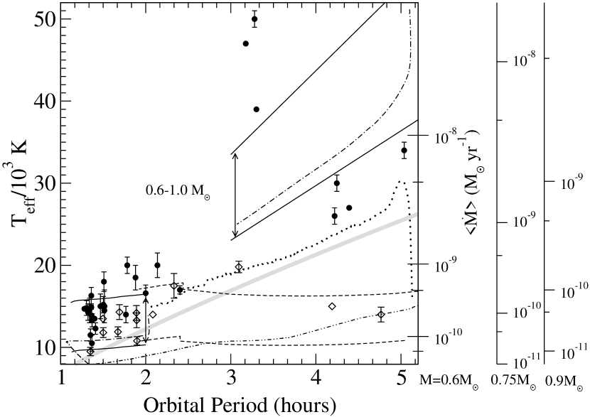
Figure 5.— Observed $T_{\rm eff}$ in the best observational cases (data from Table  1). Non-magnetic systems, a mix of dwarf novae and novalikes in low states, are indicated with solid circles and magnetic systems, all Polars, with open diamonds. Error bars indicate uncertainty dominated by the unknown WD mass. Points without error bars are less accurate than those with, but their uncertainty is not easily quantified. An approxmate mapping to $\langle\dot{M}\rangle$ is shown on the right vertical scale assuming $M=0.75M_{\odot}$, $0.6M_{\odot}$ or $0.9M_{\odot}$ as indicated. The empirical relation of Patterson (1984; thick grey line) is shown, along with several theoretical predictions: traditional magnetic braking (Howell et al. 2001; between solid lines, dot-dashed line), Andronov et al. (2003; dot-dot-dash line), Ivanova & Taam (2004; dotted line), and evolution under only gravitational radiation losses (between dashed lines). There is a clear demonstration that, for $P_{\rm orb}>3$ hours, stellar wind angular momentum loss is inhibited in the strongly magnetic systems.

5. Discussion

While we will now inspect the values listed in Table 1 for possible correlations, we must be utterly aware of the fact that the set of known CVWD temperatures is subject to severe selection effects. A very obvious, but crucial statement is that we need to be able to see the WD in order to measure its temperature, and, as mentioned above, this is not, or only marginally the case in systems where the mass transfer rate is too high. Therefore, it is possible that the temperatures obtained are rather lower limits than average values, as WDs in systems with higher accretion rates will be hotter – but not visible. This is most likely a stronger bias above the orbital period gap than below.

Our collection of secure $T_{\rm eff}$ measurements as listed in Table 1 are plotted against system $P_{\rm orb}$ in Figure 5. Non-magnetic (solid circles) and strongly magnetic (open diamonds) systems are differentiated by symbol type. For the highest quality measurements, the uncertainty in $T_{\rm eff}$, which is dominated by the unknown WD mass, is indicated with an error bar. Note that this means points without error bars are less accurate than those with, but their uncertainty is not easily quantified. An approximate $\langle\dot{M}\rangle$ scale is shown on the right if an expected typical mass (0.75$M_{\odot}$; Smith & Dhillon 1998; Knigge 2006) is chosen, but the degree of scatter expected is essentially unknown. We show for comparison the empirical relation of Patterson (1984), using an assumed primary mass of $M=0.75M_{\odot}$. From our $T_{\rm eff}$ data we infer modestly higher mass transfer rates at all orbital periods, although a higher average mass is also a viable explanation.

It is useful to dislay a variety of theoretical predictions to compare with our data. Solid lines show the $T_{\rm eff}$ range expected for the $\langle\dot{M}\rangle$ obtained from typical interrupted magnetic braking scenarios, for the mass range 0.6 to $0.9M_{\odot}$ (see Howell et al. 2001 and references therein). Here we have used the mass-radius relation for the donor star in the study by Kolb & Baraffe (1999) for below the period gap and above the gap a value of $\langle\dot{M}\rangle=10^{-9}M_{\odot}$ at $P_{\rm orb}=3$ hours and $10^{-8}M_{\odot}$ yr^-1 at $P_{\rm orb}=6$ hours, with a line between. Also shown is a curve (dot-dashed) for the $M=0.7M_{\odot}$ history from Howell et al. (2001). The relation of Andronov et al. (2003) for an unevolved donor is also shown, but implies much lower $\langle\dot{M}\rangle$ than the data support. The mass-transfer history of a case utilizing the weaker braking law posited by Ivanova & Taam (2004) is shown by the dotted line. This curve corresponds to their $\langle\dot{M}\rangle$ history for a $0.8M_{\odot}$ donor and a $0.6M_{\odot}$ primary, but for display purposes we have used $M=0.75M_{\odot}$ for the primary mass to obtain the $T_{\rm eff}$, thus the true predicted $T_{\rm eff}$ is likekly slightly higher. For comparison to the magnetic systems, we have used the main sequence mass-radius relation given by Howell et al. (2001) to determine $\langle\dot{M}\rangle$ for non-conservative mass transfer under gravitational radiation only. The resulting $T_{\rm eff}$ is shown by dashed lines, again for the mass range 0.6 to $0.9M_{\odot}$.

Uncertainty and caveats due to selection bias will be discussed below, as will the contrast between magnetic and non-magnetic systems. Comparing our measurements for non-magnetic systems to the predictions shows that we infer mass transfer rates that are lower than the predictions of traditional magnetic braking. Assuming that there is no strong selection bias toward lower $\langle\dot{M}\rangle$ systems, not a trivial assumption as discussed below, our data above the period gap are more consistent with the weakened angular momentum loss proposed by Ivanova & Taam (2004), though still a bit higher than their predictions. The angular momentum law in the traditional magnetic braking picture was largely calibrated in order to raise the radius of the companion enough to reproduce the period gap, and, by virtue of this fact, evolution following the Ivanova & Taam (2004) relation might lack an appropriate period gap. The consistency of our data with the ”softer” law of Ivanova & Taam (2004) and the presence of the high-$\langle\dot{M}\rangle$ VY Scl systems, suggest a very different picture, where the bloating of the companion might be localized to just above the period gap. There remains much room for improvement in the development of braking laws, as current laws remain fairly empirical with only modest input from understanding of the magnetospheric structure and even less from possible properties of the stellar dynamo.

5.1. Uncertainty, Scatter, and Bias

We would like to utilize our collection of $T_{\rm eff}$ measurements mainly to constrain the dependence of $\langle\dot{M}\rangle$ on $P_{\rm orb}$ and thereby evaluate angular momentum loss laws utilized to predict this relation in CV evolution. There are two important sources of general uncertainty bearing on conclusions drawn from this dataset, which follow from the discussions of previous sections: (1) uncertainty due to the effects of long-term $\dot{M}$ variations on $T_{\rm eff}$, and (2) uncertainty due to inaccessibility of quiescent $T_{\rm eff}$ measurements at a given $P_{\rm orb}$. Each of these will introduce qualifications to the naive interpretation that $L_{\rm q}$ can be converted directly into $\langle\dot{M}\rangle$ representative of that $P_{\rm orb}$ interval for that kind of system (magnetic or non-magnetic) via a relation like equation 1.

5.1.1 Long-term $\dot{M}$ Variations

Given only a single $T_{\rm eff}$ measurement, it is always possible that $\langle\dot{M}\rangle$ is something other than that implied by $T_{\rm eff}$, and we are observing a transient state. However, we do not have only one $T_{\rm eff}$ measurement; we have multiple measurements for objects in each of the 3 classes discussed in section 4: dwarf novae, novalikes displaying low states, and polars. In light of the time series and analysis of section 2, medium-term variations in $\dot{M}$, on scales of hundreds to thousands of years, would manifest as object-to-object scatter in $T_{\rm eff}$ at a given $P_{\rm orb}$. In contrast, the measurements of $T_{\rm eff}$ are remarkably consistent for the groups. The novalikes show the best evidence of scatter, and therefore of $\dot{M}$ variations on these timescales. They also would have the shortest adjustment time for their $T_{\rm eff}$ due to the large implied $\langle\dot{M}\rangle$ and luminosities. Thus novalikes displaying low states might accrete at $\simeq 10^{-8}M_{\odot}$ yr^-1 for periods of 100 years or so, and but have $\langle\dot{M}\rangle$ of more like a few $10^{-9}M_{\odot}$ yr^-1. This can be better quantified as more measurements become available.

The consistency of the $T_{\rm eff}$ values at a given $P_{\rm orb}$ within each group provides good evidence against large, medium-term variations in $\dot{M}$. For the $\langle\dot{M}\rangle$ appropriate for objects with $T_{\rm eff}\lesssim 20$kK, this statement extends to even $10^{5}$ years or more. That is, the objects for which we have good measurements of $T_{\rm eff}$ appear to have remarkably similar $\dot{M}$ histories over the last $10^{3}$ to $10^{5}$ years, though these objects were likely to have been born at a variety of $P_{\rm orb}$’s. As noted earlier, a true scatter is expected due to variations in $M_{\rm acc}$ and $M$ among observed systems. This makes the consistency among the measurements even more remarkable; enough to suggest there might be some mechanism, possibly in Classical Nova outbursts, which regulates $M$ beyond just selection bias. More careful treatment of sample bias, in particular with respect to the WD mass, which actually entails more uniform UV study of known systems, would be necessary to make conclusions on the presence or absence of such a mechanism.

The extreme case of uncertainty due to long term $\dot{M}$ variations arises from the fact that inactive systems, as e.g. in the hibernation scenario of Shara et al. (1986) or in irradiation-induced mass transfer cycles (Ritter et al., 2000), may not be included in the CV census at all, and therefore there is no opportunity to measure their $T_{\rm eff}$. This can be roughly quantified by considering a system with a duty cycle $f$, which is active for a time period $t_{\rm active}$ and then ceases mass transfer for a period of $t_{\rm active}(1-f)/f$. During the active phase, the $L_{\rm q}$ of such a system is given approximately by

$$L_{\rm q,active}\approx L_{\rm q}(\langle\dot{M}\rangle)+\delta L_{\rm q}(\dot{M}_{\rm active},t_{\rm active})$$ (6)

where the dependence of $\delta L_{\rm q}$ on $t_{\rm active}$ is the same as the dependence on thermal time shown in Figure 2. We introduce a fractional response function $R_{L}$ such that $\delta L_{\rm q}(\dot{M}_{\rm active},t_{\rm active})=L_{\rm q}(\dot{M}_{\rm active})\cdot R_{L}(t_{\rm active})$ such that $0\leq R_{L}\leq 1$. Then $R_{L}(t_{\rm active})$ is the fractional response to an order unity variation in $\dot{M}$ on a timescale $t_{\rm active}$, which increases with $t_{\rm active}$, and is the unitless quantity actually shown in Figure 2. Noting that $\dot{M}_{\rm active}\approx\langle\dot{M}\rangle/f$ and that $L_{\rm q}\propto\dot{M}$, we have

$$L_{\rm q,active}\approx L_{\rm q}(\langle\dot{M}\rangle)\cdot(1+R_{L}(t_{\rm active})/f)\ .$$ (7)

This demonstrates that for short $t_{\rm active}$, such that $R_{L}\ll 1$, $L_{\rm q,active}$ provides a good proxy for $L_{\rm q}(\langle\dot{M}\rangle)$, and therefore $T_{\rm eff}$ is a good indicator of $\langle\dot{M}\rangle$ even with a direct conversion. However, for $R_{L}(t_{\rm active})\sim 1$ and small $f$, $L_{\rm q}$ during the active state can be largely unrelated to $\langle\dot{M}\rangle$, and instead be set by $f\approx\langle\dot{M}\rangle/\dot{M}_{\rm active}$ and $t_{\rm active}$. It should be noted that a long $t_{\rm active}$ and a low $f$ can imply a very long recurrence time.

The low duty cycle and long recurrence time scenario just described is very unlikely to apply to systems with $T_{\rm eff}\lesssim 20$kK. The proximity of the $\langle\dot{M}\rangle$ implied for these systems to the lower limit set by gravitational radiation angular momentum losses (dashed lines in figure 5) excludes $f\ll 1$. This means that time series like those presented in Section 2.4, where $f=0.5$, are appropriate for these systems. Additionally, as discussed above, very long $t_{\rm active}\gtrsim 10^{6}$ years would be necessary to ensure consistency among so many independent objects.

The situation for non-magnetic systems above the period gap is less constraining. Assuming that there is some mechanism which can regulate $\dot{M}_{\rm active}$ with some precision, the consistency of several measurements in this region implies that $t_{\rm active}$ must at least be a few times the time it takes to reach $L_{\rm q}(\dot{M}_{\rm active})$. From the higher $\langle\dot{M}\rangle$ curve in Figure 2, it will take approximately 5,000 years to rise within 20% of the $L_{\rm q}(\dot{M}_{\rm active})$ indicated for these systems, so that we can estimate $t_{\rm active}\gtrsim 10^{4}$ years. In this case we are assuming that $R_{L}(t_{\rm active})\simeq 1$, so that in order to overestimate the $\langle\dot{M}\rangle$ by a factor of $10$ requires $f=1/10$, and thus a recurrence time of $10^{5}$ years and a similar duration of the inactive phase. Thus long-timescale hibernation scenarios (e.g. Shara et al., 1986) cannot be excluded by the current $T_{\rm eff}$ data. There is also no apparent evidence favoring such scenarios, in the form of downward scatter of objects still transiting between inactive and active phases.

A sample of $T_{\rm eff}$ measurements for detached systems in the 3-6 hour $P_{\rm orb}$ interval could conclusively rule this out by the absence of excess WDs with $T_{\rm eff}\simeq 15$ kK compared to longer periods. Such samples are currently being constructed and the results are ambiguous. Several detached WD+MS systems that bear the characteristics of hibernating CVs have been identified, namely BPM 71214 with $\mbox{$P_{\rm orb}$}=290$ min and $\mbox{$T_{\rm eff}$}=17\,000$ K, (Kawka et al., 2002; Kawka & Vennes, 2003), EC 13471–1258 with $\mbox{$P_{\rm orb}$}=217$ min and $\mbox{$T_{\rm eff}$}=14\,220\pm 350$ K (O’Donoghue et al., 2003), and HS 2237+8154 with $\mbox{$P_{\rm orb}$}=178$ min and $\mbox{$T_{\rm eff}$}=11\,500$ K (Gänsicke et al., 2004a). The first two show promise, however there is significant selection bias toward finding hot WDs and there is an expected (contaminant) population of systems which are just coming into contact and simply have young WD primaries.

5.1.2 Inaccessible Quiescent $T_{\rm eff}$ Values

The second major source of uncertainty in drawing conclusions from the available set of $T_{\rm eff}$ measurements is due to the set of circumstances which must come to pass in order to allow direct measurement of the WD photosphere. For Dwarf Novae, which accrete in bursts with $\dot{M}\gg\langle\dot{M}\rangle$, it is also necessary to wait a sufficient period of time after the outburst in order to get a good idea of the baseline quiescent $T_{\rm eff}$ that is escaping from the deeper layers of the envelope with longer thermal times. As mentioned above, this latter can be achieved largely empirically by selecting the timing of $T_{\rm eff}$ measurements with respect to disk outbursts.

Non-magnetic Cataclysmic variables with $P_{\rm orb}<2$ hours are predominantly Dwarf Novae (Ritter & Kolb, 2003). The selection criteria for such systems are important: the emission of unknown origin discussed in section 4.1 must be less bright than the WD in the UV, and the absorption of the system must be low enough that the WD can be measured well, placing a constraint on the inclination of the system. Without better characterization of the unidentified broad-band emission, our only option is to assume it is a random contaminant which is uncorrelated with $\langle\dot{M}\rangle$. Again, it is possible to confirm this with better UV study of known systems. Since both of these selection criteria are not expected to correlate with $\langle\dot{M}\rangle$, we believe that our sample of non-magnetic systems in the $P_{\rm orb}<2$ hour range should be representative of the typical $\langle\dot{M}\rangle$ in these systems. There might be a slight bias toward low $\langle\dot{M}\rangle$ due to their having more accessible quiescent intervals, but there are no indications that this is the case.

For $P_{\rm orb}>3$ hours, DN are a minority of the population, and thus there is concern that only particular systems with low $\langle\dot{M}\rangle$ have made it into our sample. If true, this would imply that the region at higher $T_{\rm eff}$ than the measured systems in the 3.5-5 hour period range in Figure 5 should contain the higher $\langle\dot{M}\rangle$ systems which did not enter our sample. This would imply a higher $\langle\dot{M}\rangle$ than we can infer directly from the measured systems, and thus impart more favor to the traditional magnetic braking prescriptions.

5.2. VY Sculptoris stars

The three VY Scl stars with well-determined temperatures stand out in the 3–4 h period range containing the hottest CVWDs known, and consequently have very high mass transfer rates. In effect, the deduced mass transfer rates exceed those predicted by the standard evolution theory for the majority of CVs within that period range (Kolb, 1993; Howell et al., 2001). $T_{\rm eff}$ measurements of VY Scl require the fairly prompt observational attention once they enter a low state, preferably with an UV facility, which explains the small number of available values. Practically all VY Scl stars are located within the 3–4 h orbital period range (e.g. Honeycutt & Kafka, 2004). Furthermore, Rodríguez-Gil et al. (2007) have shown that the SW Sex stars, intrinsically bright novalike variables which are intimately related to the VY Scl stars (Hameury & Lasota 2002; Hellier 2000; in fact, the two groups overlap to a large extent) are the dominant population of CVs in the 3–4 h orbital period range. Speculating that high $T_{\rm eff}$ and $\langle\dot{M}\rangle$ are a common characteristic to all VY Scl/SW Sex stars suggests that these systems represent an exceptional phase in CV evolution. One possible explanation is that these are systems that just evolved into a semi-detached configuration, as the the mass transfer goes through a short peak during turn-on (e.g. D’Antona et al., 1989), and that CVs are preferentially born within the 3–4 h period range, which would be the case if the initial mass distribution is peaked towards equal masses in the progenitor main-sequence binaries (de Kool, 1992).

5.3. Polars and Wind Braking

In agreement with the interrupted magnetic braking scenario for non-magnetic CV evolution, these $T_{\rm eff}$ measurements indicate that $\langle\dot{M}\rangle$ is approximately an order of magnitude larger above the period gap than below. But $T_{\rm eff}$ measurements can do better than this. Knowing the relation between $T_{\rm eff}$ and $\langle\dot{M}\rangle$ we can say that the objects below the gap are roughly consistent with gravitational radiation losses, with possibly some enhancement of a factor of 2 or 3 for non-magnetic systems. In contrast $\langle\dot{M}\rangle$ above the period gap is an order of magnitude greater than that predicted by gravitational radiation alone. There is, finally, an additional constraint that is entirely specific to the magnetic braking mechanism: we find a marked difference between the $\langle\dot{M}\rangle$ implied for non-magnetic systems and those of strongly magnetic systems (Polars) and, as shown in Figure 5, the $\langle\dot{M}\rangle$ in Polars is consistent with that expected from gravitational radiation angular momentum loss alone, while that in non-magnetic systems is at least an order of magnitude higher. As shown in section 3.2 such a decrement in $T_{\rm eff}$, which is measured away from the poles where the accretion impacts, is too large to be explained by accretion geometry for the magnetic fields observed. Additionally, from the discussion in section 5.1.1, such a large difference would require an extreme assumption about the duty cycle in non-magnetic systems. Therefore the contrast between magnetic and non-magnetic systems must arise from a difference in $\langle\dot{M}\rangle$.

The lack of an enhanced $\langle\dot{M}\rangle$ in magnetic systems arises from changes in the magnetic field structure near the secondary which hinders the loss of angular momentum via a wind (Li et al., 1994b). Our measurements provide the best direct evidence that this does occur, and additionally that the resulting $\langle\dot{M}\rangle$ is consistent with gravitational radiation. This provides very strong support for the basic picture of magnetic braking, though the precise mechanism by which it ceases is still somewhat mysterious. We should highlight that this reduction of magnetic braking in Polars is widely expected, and was originally proposed to explain the lack of an apparent period gap in magnetic CVs (Wickramasinghe & Wu, 1994; Li et al., 1994a; Webbink & Wickramasinghe, 2002). The resulting slower evolution of magnetic systems will also enhance the number of magnetic CVs relative to nonmagnetic ones with respect to field WDs, giving roughly the fraction observed (Townsley & Bildsten, 2005).

5.4. Below the Period Gap

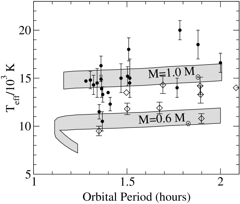
Figure 6.— Closeup of $P_{\rm orb}<2$ hours, filled circles indicate non-magnetic systems and open diamonds indicate magnetic systems (see Figure 5). Overplotted are the range of $T_{\rm eff}$ expected for accretion driven by gravitational radiation (Kolb & Baraffe, 1999) for two WD masses. Note that the theoretical minimum period is notably shorter than that inferred from the data.

Due to the need for low $\langle\dot{M}\rangle$, many of of the high-quality $T_{\rm eff}$ measurements are for systems with $P_{\rm orb}<2$ hours. An expanded plot of this region is shown in Figure 6. For $M=0.6M_{\odot}$ we use the $\langle\dot{M}\rangle$ from Kolb & Baraffe (1999) directly and for $1.0M_{\odot}$ we use their $M$-$R$ relation for the secondary and gravitational radiation angular momentum losses. We display the predicted region for $0.05M_{\rm ign}<M_{\rm acc}<0.95M_{\rm ign}$ which object will traverse during buildup toward a classical nova when $M_{\rm acc}=M_{\rm ign}$. Many of the measurements for non-magnetic objects are clustered about $T_{\rm eff}=15$ kK, providing evidence, as discussed above, against long-term $\dot{M}$ variations. The exception to this is that there is significant downward scatter at the shortest orbital periods 1.3-1.4 hours. The presence of this scatter at these $P_{\rm orb}$ and not at slightly longer ones strongly suggests that the $\langle\dot{M}\rangle$ in these objects has begun to decline as expected when they pass beyond period minimum (Howell et al., 2001). This feature highlights the disagreement of the observed period minimum and that predicted by theory (Kolb & Baraffe, 1999), which is apparent in Figure 6 because the minimum is not very sensitive to $M$. As discussed in Townsley & Bildsten (2003) we find that either short-period CVs have $M\simeq 0.9$-$1.0M_{\odot}$ (such as e.g. found in SDSS 1035+0555, Littlefair et al. (2006b)) or mass transfer is enhanced by a factor of 2-3 over that predicted by only gravitational radiation losses. There is also some evidence from the few measurements near $P_{\rm orb}=1.8$ hours that the dependence of $\langle\dot{M}\rangle$ on $P_{\rm orb}$ is not as flat as is predicted by gravitational radiation. More measurements will be necessary before conclusions can be drawn.

Even here below the period gap there is a smaller but significant difference between strongly magnetic and non-magnetic systems. The energy released by compression deeper than the point at which the material is able to spread over the star amounts to better than 80% of the $L_{\rm q}$ expected in the non-magnetic case. However such a decrease in $L_{\rm q}$ only reduces $T_{\rm eff}$ from 15 kK to 14 kK, not enough to account for the difference in $T_{\rm eff}$ between magnetic and non-magnetic systems below the gap. For high-field cases, $B\simeq 10^{8}$ G, the reduction can reach 50%, bringing $T_{\rm eff}$ down to 13 kK. However, none of the systems used in this paper (Table 1) has such a high field (see Sect. 4.3). It still appears that either $\langle\dot{M}\rangle$ is slightly above that due to gravitational radiation or these magnetic objects do have typical $M\simeq 0.7M_{\odot}$. A typical mass above $0.6M_{\odot}$ is expected both from simple selection bias because the luminosity increases with $M$ and since field magnetic WDs tend to be higher mass than non-magnetics.

Appendix A Simulation of hydrostatic envelope in plane parallel

In this appendix we detail our treatment via simulation of the envelope of the accreting WD. We work in the plane parallel, hydrostatic approximation so that $P=gy$ at every point. Discretizing the temperature in $y$ and time, the heat equation, (3), is integrated forward in time using a Crank-Nicholson like integration rule

$$\frac{T^{n+1}_{k}-T^{n}_{k}}{t_{n+1}-t_{n}}=\frac{1}{2}\left[\left.\frac{\partial T}{\partial t}\right|_{t_{n},y_{k}}+\left.\frac{\partial T}{\partial t}\right|_{t_{n+1},y_{k}}\right]$$ (A1)

where the derivatives of $T$ in $y$ on the grid are evaluated via centered differences

$$\left.\frac{\partial T}{\partial y}\right|_{y_{k}}=\frac{T_{k+1}-T_{k-1}}{y_{k+1}-y_{k-1}},\quad\quad\left.\frac{\partial^{2}T}{\partial y^{2}}\right|_{y_{k}}=\frac{T_{k+1}-T_{k}}{y_{k+1}-y_{k}}-\frac{T_{k}-T_{k-1}}{y_{k}-y_{k-1}}.$$ (A2)

Initial conditions are taken from the static models used by TB04. Note that eq. (A1) is an implicit integration rule, representing $N$ equations in $N$ unknowns, which is solved for $T_{k}^{n+1}$ using a Newton-Raphson iteration. Timesteps are chosen such that the maximum $\Delta T/T$ at any point on the grid is less that $10^{-3}$. The steady state solution produced by the time-dependent code compares very well with the static solutions produced by direct integration of the structure equations in TB04.

The flux at the outer boundary is found by integrating eq. (3) in from the photosphere using a 4th order Runge-Kutta integrator. A shooting method (root-find) is used to vary $F_{\rm photosphere}$ to match $T(y_{\rm outer})$ at the outer edge of the simulation grid, $y_{\rm outer}$, and the resulting $F(y_{\rm outer})$ is used for the flux at the edge of the grid. While there are no convection zones in the simulation domain, there is a convection zone in the part of the envelope which forms the boundary condition. Convection here is treated with the ML2 formalism (Bergeron et al., 1992). Use of this boundary condition is equivalent to the approximation that the thermal time of the layer of depth $y_{\rm outer}$ is negligible. The inner boundary condition is constant temperature, fixed to the equilibrium temperature at the $\langle\dot{M}\rangle$ under consideration (TB04).

Two different grids are used in this work. For the long-timescale variation studies of section 2.4, we use $N=120$ points evenly spaced in $\log y$ extending from from $y=6\times 10^{5}$ g cm^-2 to $3.9\times 10^{12}$ g cm^-2, corresponding to mass coordinates of $1.6\times 10^{-9}M_{\odot}$ and $0.01M_{\odot}$, respectively on a $0.9M_{\odot}$ WD, $R=6.45\times 10^{8}$ cm. For $\langle\dot{M}\rangle=5\times 10^{-11}M_{\odot}$ yr^-1 at this mass, the thermal timescale of the outermost point $t_{\rm th}(y_{\rm outer})\simeq 10$ days, much shorter than any variability being studied. For the study of TT Ari in section 3, the upper edge of the grid was extended to shorter thermal timescales. In this case we used 100 points between $y=2.75\times 10^{4}$ and $3.64\times 10^{8}$ g cm^-2 and 50 points extending down to $3.9\times 10^{12}$ g cm^-2, for a total 150. This outer point corresponds to $t_{\rm th}(y_{\rm outer})\simeq 15$ hours for the parameters used to reproduce TT Ari.

The depth of the boundary between the solar abundance accreted material and the underlying 50/50 carbon and oxygen material, $y_{\rm HHe}=M_{\rm acc}/(4\pi R^{2})$ is tracked with a separate variable whose evolution is directly specified from $\dot{M}(t)$. Although selecting between two compositions depending upon whether $y_{k}<y_{\rm HHe}$ or $y_{\rm HHe}<y_{k}$ gives suitably accurate results, a smooth progression is significantly more easily integrated numerically. This allows a smooth change in abundance at a given point while still allowing a sharp interface to be represented on a modest resolution grid. We now proceed to describe our interface treatment in detail.

Consider the interface as being at column depth $y_{I}=y_{\rm HHe}$ lying between two gridpoints at depths $y_{k}$ and $y_{k+1}$. The temperature at each of these points is $T_{k}$ and $T_{k+1}$ respectively, and that at the interface is $T_{I}$. Both the temperature and flux must be continuous at the interface, so letting $F_{H}$ and $F_{C}$ indicate the flux evaluated at $y_{I}$ on the H/He side and the C/O side respectively, we have

$$F_{I}=\frac{4acT^{3}}{3\kappa}\frac{\partial T}{\partial y}=F_{H}=F_{C}\quad{\rm or}\quad\frac{1}{\kappa_{H}(y_{I},T_{I})}\left(\frac{\partial T}{\partial y}\right)_{H}=\frac{1}{\kappa_{C}(y_{I},T_{I})}\left(\frac{\partial T}{\partial y}\right)_{C}$$ (A3)

where the subscripts $H$ and $C$ on the derivatives indicate evaluation on respective sides of the interface and on $\kappa$ indicate evaluation at $P_{I}$ and $T_{I}$ but with H/He and C/O composition respectively. It is inadvisable to attempt to solve for $T_{I}$ directly because $y_{I}-y_{k}$ can become arbitrarily small and lead to singularities. Instead we will solve for the derivatives. The interface temperature can be written by expanding from both directions

$$T_{I}=T_{k}+(y_{I}-y_{k})\left(\frac{\partial T}{\partial y}\right)_{H}=T_{k+1}+(y_{I}-y_{k+1})\left(\frac{\partial T}{\partial y}\right)_{C}$$ (A4)

which upon combination with eq. (A3) gives

$$0=T_{k+1}-T_{k}+\left[(y_{I}-y_{k+1})\frac{\kappa_{C}(T_{I})}{\kappa_{H}(T_{I})}-(y_{I}-y_{k})\right]\left(\frac{\partial T}{\partial y}\right)_{H}\ .$$ (A5)

By using the first expression for $T_{I}$ from (A4), this can be solved for $(\partial T/\partial y)_{H}$.

Finally, all the derivatives near the interface can then be constructed from the grid quantities and $(\partial T/\partial y)_{H}$ in a way which mimics centered differencing. We let $(\frac{\partial T}{\partial y})_{H}$ stand in for the first order difference at the midpoint between $k$ and $k+1$, since it should be approximately what that first order difference would have been if there were no change in composition. This gives

$$\left(\frac{dT}{dy}\right)_{k} = \frac{1}{2}\left[\left(\frac{\partial T}{\partial y}\right)_{H}+\frac{T_{k}-T_{k-1}}{y_{k}-y_{k-1}}\right]\ ,$$ (A6)

$$\left(\frac{d^{2}T}{dy^{2}}\right)_{k} = \frac{2}{y_{k+1}-y_{k-1}}\left[\left(\frac{\partial T}{\partial y}\right)_{H}-\frac{T_{k}-T_{k-1}}{y_{k}-y_{k-1}}\right]\ ,$$ (A7)

$$\left(\frac{dT}{dy}\right)_{k+1} = \frac{1}{2}\left[\frac{T_{k+2}-T_{k+1}}{y_{k+2}-y_{k+1}}+\left(\frac{\partial T}{\partial y}\right)_{C}\right]\ ,$$ (A8)

$$\left(\frac{d^{2}T}{dy^{2}}\right)_{k+1} = \frac{2}{y_{k+2}-y_{k}}\left[\frac{T_{k+2}-T_{k+1}}{y_{k+2}-y_{k+1}}-\left(\frac{\partial T}{\partial y}\right)_{C}\right]\ .$$ (A9)

For the outer portions of the envelope we use the 2002 update to the OPAL equation of state tables (Rogers et al., 1996), and for higher densities we use the analytical approximations for a fully ionized plasma from Paczyński (1983) and Coulomb correction from Chabrier & Potekhin (1998). While these two EOS methods are very consistent at the table edge, a linear average in a crossover region of a factor of 5 in density is used to smooth the boundary. OPAL radiative opacities (Iglesias & Rogers, 1996) are also used along with conductivities from Itoh et al. (1983).

References

- Andronov et al. (2003) Andronov, N., Pinsonneault, M., & Sills, A. 2003, ApJ, 582, 358
- Araujo-Betancor et al. (2005a) Araujo-Betancor, S., Gänsicke, B. T., Hagen, H.-J., Marsh, T. R., Harlaftis, E. T., Thorstensen, J., Fried, R. E., Schmeer, P., & Engels, D. 2005a, A&A, 430, 629
- Araujo-Betancor et al. (2005b) Araujo-Betancor, S., Gänsicke, B. T., Long, K. S., Beuermann, K., de Martino, D., Sion, E. M., & Szkody, P. 2005b, ApJ, 622, 589
- Araujo-Betancor et al. (2003) Araujo-Betancor, S., Knigge, C., Long, K. S., Hoard, D. W., Szkody, P., Rodgers, B., Krisciunas, K., Dhillon, V. S., Hynes, R. I., Patterson, J., & Kemp, J. 2003, ApJ, 583, 437
- Belle et al. (2003) Belle, K. E., Howell, S. B., Sion, E. M., Long, K. S., & Szkody, P. 2003, ApJ, 587, 373
- Bergeron et al. (1992) Bergeron, P., Wesemael, F., & Fontaine, G. 1992, ApJ, 387, 288
- Beuermann (2006) Beuermann, K. 2006, A&A, 460, 783
- Beuermann et al. (1998) Beuermann, K., Baraffe, I., Kolb, U., & Weichhold, M. 1998, A&A, 339, 518
- Beuermann et al. (2004) Beuermann, K., Harrison, T. E., McArthur, B. E., Benedict, G. F., & Gänsicke, B. T. 2004, A&A, 419, 291
- Beuermann et al. (2000) Beuermann, K., Wheatley, P., Ramsay, G., Euchner, F., & Gänsicke, B. T. 2000, A&A, 354, L49
- Chabrier & Potekhin (1998) Chabrier, G. & Potekhin, A. Y. 1998, Phys. Rev. E, 58, 4941
- Cheng et al. (2000) Cheng, F. H., Horne, K., Marsh, T. R., Hubeny, I., & Sion, E. M. 2000, ApJ, 542, 1064
- D’Antona et al. (1989) D’Antona, F., Mazzitelli, I., & Ritter, H. 1989, A&A, 225, 391
- de Kool (1992) de Kool, M. 1992, A&A, 261, 188
- de Martino et al. (2006) de Martino, D., Bonnet-Bidaud, J.-M., Mouchet, M., Gänsicke, B. T., Haberl, F., & Motch, C. 2006, A&A, 449, 1151
- Dhillon et al. (2007) Dhillon, V. S., Marsh, T. R., Stevenson, M. J., Atkinson, D. C., Kerry, P., Peacocke, P. T., Vick, A. J. A., Beard, S. M., Ives, D. J., Lunney, D. W., McLay, S. A., Tierney, C. J., Kelly, J., Littlefair, S. P., Nicholson, R., Pashley, R., Harlaftis, E. T., & O’Brien, K. 2007, MNRAS, 378, 825
- Eisenbart et al. (2002) Eisenbart, S., Beuermann, K., Reinsch, K., & Gänsicke, B. T. 2002, A&A, 382, 984
- Epelstain et al. (2007) Epelstain, N., Yaron, O., Kovetz, A., & Prialnik, D. 2007, MNRAS, 374, 1449
- Eracleous et al. (1994) Eracleous, M., Horne, K., Robinson, E. L., Zhang, E.-H., Marsh, T. R., & Wood, J. H. 1994, ApJ, 433, 313
- Faulkner (1971) Faulkner, J. 1971, ApJ, 170, L99+
- Feline et al. (2004) Feline, W. J., Dhillon, V. S., Marsh, T. R., Stevenson, M. J., Watson, C. A., & Brinkworth, C. S. 2004, MNRAS, 347, 1173
- Feline et al. (2005) Feline, W. J., Dhillon, V. S., Marsh, T. R., Watson, C. A., & Littlefair, S. P. 2005, MNRAS, 364, 1158
- Gänsicke et al. (2001) Gänsicke, B. T., Schmidt, G. D., Jordan, S., & Szkody, P. 2001, ApJ, 555, 380
- Gänsicke et al. (2005) Gänsicke, B. T., Szkody, P., Howell, S. B., & Sion, E. M. 2005, ApJ, 629, 451
- Gänsicke (1999) Gänsicke, B. T. 1999, in Annapolis Workshop on Magnetic Cataclysmic Variables, ed. C. Hellier & K. Mukai (ASP Conf. Ser. 157), 261–272
- Gänsicke et al. (2004a) Gänsicke, B. T., Araujo-Betancor, S., Hagen, H.-J., Harlaftis, E. T., Kitsionas, S., Dreizler, S., & Engels, D. 2004a, A&A, 418, 265
- Gänsicke & Beuermann (1996a) Gänsicke, B. T. & Beuermann, K. 1996a, in Röntgenstrahlung from the Universe, ed. H. U. Zimmermann, J. Trümper, & H. Yorke, MPE Report No. 263 (Garching: MPE), 137–138
- Gänsicke & Beuermann (1996b) Gänsicke, B. T. & Beuermann, K. 1996b, A&A, 309, L47
- Gänsicke et al. (1995) Gänsicke, B. T., Beuermann, K., & de Martino, D. 1995, A&A, 303, 127
- Gänsicke et al. (2000) Gänsicke, B. T., Beuermann, K., de Martino, D., & Thomas, H.-C. 2000, A&A, 354, 605
- Gänsicke et al. (2004b) Gänsicke, B. T., Jordan, S., Beuermann, K., de Martino, D., Szkody, P., Marsh, T. R., & Thorstensen, J. 2004b, ApJ, 613, L141
- Gänsicke & Koester (1999) Gänsicke, B. T. & Koester, D. 1999, A&A, 346, 151
- Gänsicke et al. (2006) Gänsicke, B. T., Long, K. S., Barstow, M. A., & Hubeny, I. 2006, ApJ, 639, 1039
- Gänsicke et al. (1999) Gänsicke, B. T., Sion, E. M., Beuermann, K., Fabian, D., Cheng, F. H., & Krautter, J. 1999, A&A, 347, 178
- Gänsicke et al. (2001) Gänsicke, B. T., Szkody, P., Sion, E. M., Hoard, D. W., Howell, S., Cheng, F. H., & Hubeny, I. 2001, A&A, 374, 656
- Godon et al. (2006) Godon, P., Seward, L., Sion, E. M., & Szkody, P. 2006, AJ, 131, 2634
- Godon et al. (2004) Godon, P., Sion, E. M., Cheng, F., Gänsicke, B. T., Howell, S., Knigge, C., Sparks, W. M., & Starrfield, S. 2004, ApJ, 602, 336
- Greenstein (1957) Greenstein, J. L. 1957, ApJ, 126, 23
- Haberl et al. (2002) Haberl, F., Motch, C., & Zickgraf, F.-J. 2002, A&A, 387, 201
- Hameury et al. (1983) Hameury, J. M., Bonazzola, S., Heyvaerts, J., & Lasota, J. P. 1983, A&A, 128, 369
- Hameury et al. (1988) Hameury, J. M., King, A. R., Lasota, J. P., & Ritter, H. 1988, MNRAS, 231, 535
- Hameury & Lasota (2002) Hameury, J. M. & Lasota, J. P. 2002, A&A, 394, 231
- Harrison et al. (2004) Harrison, T. E., Johnson, J. J., McArthur, B. E., Benedict, G. F., Szkody, P., Howell, S. B., & Gelino, D. M. 2004, AJ, 127, 460
- Hartley et al. (2005) Hartley, L. E., Long, K. S., Froning, C. S., & Drew, J. E. 2005, ApJ, 623, 425
- Heise & Verbunt (1988) Heise, J. & Verbunt, F. 1988, A&A, 189, 112
- Hellier (2000) Hellier, C. 2000, New Astronomy Review, 44, 131
- Hessman et al. (2000) Hessman, F. V., Gänsicke, B. T., & Mattei, J. A. 2000, A&A, 361, 952
- Hessman et al. (1989) Hessman, F. V., Koester, D., Schoembs, R., & Barwig, H. 1989, A&A, 213, 167
- Hoard et al. (2004) Hoard, D. W., Linnell, A. P., Szkody, P., Fried, R. E., Sion, E. M., Hubeny, I., & Wolfe, M. A. 2004, ApJ, 604, 346
- Honeycutt & Kafka (2004) Honeycutt, R. K. & Kafka, S. 2004, AJ, 128, 1279
- Horne et al. (1994) Horne, K., Marsh, T. R., Cheng, F. H., Hubeny, I., & Lanz, T. 1994, ApJ, 426, 294
- Howell et al. (2002) Howell, S. B., Gänsicke, B. T., Szkody, P., & Sion, E. M. 2002, ApJ, 575, 419
- Howell et al. (2001) Howell, S. B., Nelson, L. A., & Rappaport, S. 2001, ApJ, 550, 897
- Huang et al. (1996) Huang, M., Sion, E. M., Hubeny, I., Cheng, F. H., & Szkody, P. 1996, AJ, 111, 2386
- Iglesias & Rogers (1996) Iglesias, C. A. & Rogers, F. J. 1996, ApJ, 464, 943
- Itoh et al. (1983) Itoh, N., Mitake, S., Iyetomi, H., & Ichimaru, S. 1983, ApJ, 273, 774
- Ivanova & Taam (2004) Ivanova, N. & Taam, R. E. 2004, ApJ, 601, 1058
- Jordan (1992) Jordan, S. 1992, A&A, 265, 570
- Kawka & Vennes (2003) Kawka, A. & Vennes, S. 2003, AJ, 125, 1444
- Kawka et al. (2002) Kawka, A., Vennes, S., Koch, R., & Williams, A. 2002, AJ, 124, 2853
- Knigge (2006) Knigge, C. 2006, MNRAS, 373, 484
- Knigge et al. (2000) Knigge, C., Long, K. S., Hoard, D. W., Szkody, P., & Dhillon, V. S. 2000, ApJ, 539, L49
- Koester et al. (1985) Koester, D., Weidemann, V., Zeidler-K.T., E. M., & Vauclair, G. 1985, A&A, 142, L5
- Kolb (1993) Kolb, U. 1993, A&A, 271, 149
- Kolb & Baraffe (1999) Kolb, U. & Baraffe, I. 1999, MNRAS, 309, 1034
- Li et al. (1994a) Li, J. K., Wu, K. W., & Wickramasinghe, D. T. 1994a, MNRAS, 270, 769
- Li et al. (1994b) —. 1994b, MNRAS, 268, 61
- Littlefair et al. (2006a) Littlefair, S. P., Dhillon, V. S., Marsh, T. R., & Gänsicke, B. T. 2006a, MNRAS, 371, 1435
- Littlefair et al. (2006b) Littlefair, S. P., Dhillon, V. S., Marsh, T. R., Gänsicke, B. T., Southworth, J., & Watson, C. A. 2006b, Science, 314, 1578
- Livio & Pringle (1994) Livio, M. & Pringle, J. E. 1994, ApJ, 427, 956
- Long et al. (1993) Long, K. S., Blair, W. P., Bowers, C. W., Davidsen, A. F., Kriss, G. A., Sion, E. M., & Hubeny, I. 1993, ApJ, 405, 327
- Long et al. (1996) Long, K. S., Blair, W. P., Hubeny, I., & Raymond, J. C. 1996, ApJ, 466, 964
- Long et al. (2006) Long, K. S., Brammer, G., & Froning, C. S. 2006, ApJ, 648, 541
- Long et al. (2005) Long, K. S., Froning, C. S., Knigge, C., Blair, W. P., Kallman, T. R., & Ko, Y.-K. 2005, ApJ, 630, 511
- Long & Gilliland (1999) Long, K. S. & Gilliland, R. L. 1999, ApJ, 511, 916
- Long et al. (2004) Long, K. S., Sion, E. M., Gänsicke, B. T., & Szkody, P. 2004, ApJ, 602, 948
- Mateo & Szkody (1984) Mateo, M. & Szkody, P. 1984, AJ, 89, 863
- Mouchet et al. (1991) Mouchet, M., Bonnet-Bidaud, J. M., Buckley, D. A. H., & Tuohy, I. R. 1991, A&A, 250, 99
- O’Donoghue et al. (2003) O’Donoghue, D., Koen, C., Kilkenny, D., Stobie, R. S., Koester, D., Bessell, M. S., Hambly, N., & MacGillivray, H. 2003, MNRAS, 345, 506
- Paczyński (1983) Paczyński, B. 1983, ApJ, 267, 315
- Paczynski & Sienkiewicz (1981) Paczynski, B. & Sienkiewicz, R. 1981, ApJ, 248, L27
- Paczynski & Sienkiewicz (1983) —. 1983, ApJ, 268, 825
- Patterson (1984) Patterson, J. 1984, ApJS, 54, 443
- Piro et al. (2005) Piro, A. L., Arras, P., & Bildsten, L. 2005, ApJ, 628, 401
- Piro & Bildsten (2004) Piro, A. L. & Bildsten, L. 2004, ApJ, 616, L155
- Prialnik (1986) Prialnik, D. 1986, ApJ, 310, 222
- Rappaport et al. (1982) Rappaport, S., Joss, P. C., & Webbink, R. F. 1982, ApJ, 254, 616
- Rappaport et al. (1983) Rappaport, S., Verbunt, F., & Joss, P. C. 1983, ApJ, 275, 713
- Reimers & Hagen (2000) Reimers, D. & Hagen, H. J. 2000, A&A, 358, L45
- Ribas (2006) Ribas, I. 2006, Ap&SS, 304, 89
- Ritter & Kolb (2003) Ritter, H. & Kolb, U. 2003, A&A, 404, 301
- Ritter et al. (2000) Ritter, H., Zhang, Z. ., & Kolb, U. 2000, A&A, 360, 959
- Rodríguez-Gil et al. (2007) Rodríguez-Gil, P., Gänsicke, B. T., Hagen, H.-J., Araujo-Betancor, S., Aungwerojwit, A., Allende Prieto, C., Boyd, D., Casares, J., Engels, D., Giannakis, O., Harlaftis, E. T., Kube, J., Lehto, H., Martínez-Pais, I. G., Schwarz, R., Skidmore, W., Staude, A., & Torres, M. A. P. 2007, MNRAS, 377, 1747
- Rogers et al. (1996) Rogers, F. J., Swenson, F. J., & Iglesias, C. A. 1996, ApJ, 456, 902
- Rosen et al. (2001) Rosen, S. R., Rainger, J. F., Burleigh, M. R., Mittaz, J. P. D., Buckley, D. A. H., Sirk, M. M., Lieu, R., Howell, S. B., & de Martino, D. 2001, MNRAS, 322, 631
- Schmidt et al. (2005) Schmidt, G. D., Szkody, P., Vanlandingham, K. M., Anderson, S. F., Barentine, J. C., Brewington, H. J., Hall, P. B., Harvanek, M., Kleinman, S. J., Krzesinski, J., Long, D., Margon, B., Neilsen, Jr., E. H., Newman, P. R., Nitta, A., Schneider, D. P., & Snedden, S. A. 2005, ApJ, 630, 1037
- Schmidt et al. (1986) Schmidt, G. D., West, S. C., Liebert, J., Green, R. F., & Stockman, H. S. 1986, ApJ, 309, 218
- Schreiber & Gänsicke (2003) Schreiber, M. R. & Gänsicke, B. T. 2003, A&A, 406, 305
- Schwope et al. (2002) Schwope, A. D., Hambaryan, V., Schwarz, R., Kanbach, G., & Gänsicke, B. T. 2002, A&A, 392, 541
- Shafter et al. (1985) Shafter, A. W., Szkody, P., Liebert, J., Penning, W. R., Bond, H. E., & Grauer, A. D. 1985, ApJ, 290, 707
- Shara et al. (1986) Shara, M. M., Livio, M., Moffat, A. F. J., & Orio, M. 1986, ApJ, 311, 163
- Sion (1991) Sion, E. M. 1991, AJ, 102, 295
- Sion (1995) —. 1995, ApJ, 438, 876
- Sion (1999) —. 1999, PASP, 111, 532
- Sion et al. (2004) Sion, E. M., Cheng, F., Godon, P., & Szkody, P. 2004, ApJ, in press
- Sion et al. (1996) Sion, E. M., Cheng, F., Huang, M., Hubeny, I., & Szkody, P. 1996, ApJ, 471, L41
- Sion et al. (1995a) Sion, E. M., Cheng, F. H., Long, K. S., Szkody, P., Gilliland, R. L., Huang, M., & Hubeny, I. 1995a, ApJ, 439, 957
- Sion et al. (1998) Sion, E. M., Cheng, F. H., Szkody, P., Sparks, W., Gänsicke, B., Huang, M., & Mattei, J. 1998, ApJ, 496, 449
- Sion et al. (1990) Sion, E. M., Leckenby, H. J., & Szkody, P. 1990, ApJ, 364, L41
- Sion et al. (2003) Sion, E. M., Szkody, P., Cheng, F., Gänsicke, B. T., & Howell, S. B. 2003, ApJ, 583, 907
- Sion et al. (1995b) Sion, E. M., Szkody, P., Cheng, F., & Huang, M. 1995b, ApJ, 444, L97
- Sion et al. (2001) Sion, E. M., Szkody, P., Gänsicke, B., Cheng, F. H., LaDous, C., & Hassall, B. 2001, ApJ, 555, 834
- Sion & Urban (2002) Sion, E. M. & Urban, J. 2002, ApJ, 572, 456
- Smith et al. (2006) Smith, A. J., Haswell, C. A., & Hynes, R. I. 2006, MNRAS, 369, 1537
- Smith & Dhillon (1998) Smith, D. A. & Dhillon, V. S. 1998, MNRAS, 301, 767
- Southworth et al. (2006) Southworth, J., Gänsicke, B. T., Marsh, T. R., de Martino, D., Hakala, P., Littlefair, S., Rodríguez-Gil, P., & Szkody, P. 2006, MNRAS, 373, 687
- Spruit & Ritter (1983) Spruit, H. C. & Ritter, H. 1983, A&A, 124, 267
- Steeghs et al. (2007) Steeghs, D., Howell, S. B., Knigge, C., Gänsicke, B. T., Sion, E. M., & Welsh, W. F. 2007, ApJ, 667, 442
- Steeghs et al. (2001) Steeghs, D., Marsh, T., Knigge, C., Maxted, P. F. L., Kuulkers, E., & Skidmore, W. 2001, ApJ, 562, L145
- Stockman et al. (1994) Stockman, H. S., Schmidt, G. D., Liebert, J., & Holberg, J. B. 1994, ApJ, 430, 323
- Szkody et al. (2003a) Szkody, P., Anderson, S. F., Schmidt, G., Hall, P. B., Margon, B., Miceli, A., SubbaRao, M., Frith, J., Harris, H., Hawley, S., Lawton, B., Covarrubias, R., Covey, K., Fan, X., Murphy, T., Narayanan, V., Raymond, S., Rest, A., Strauss, M. A., Stubbs, C., Turner, E., Voges, W., Bauer, A., Brinkmann, J., Knapp, G. R., & Schneider, D. P. 2003a, ApJ, 583, 902
- Szkody et al. (2000a) Szkody, P., Desai, V., Burdullis, T., Hoard, D. W., Fried, R., Garnavich, P., & Gänsicke, B. 2000a, ApJ, 540, 983
- Szkody et al. (2000b) Szkody, P., Desai, V., & Hoard, D. W. 2000b, AJ, 119, 365
- Szkody et al. (2002a) Szkody, P., Gänsicke, B. T., Howell, S. B., & Sion, E. M. 2002a, ApJ, 575, L79
- Szkody et al. (2002b) Szkody, P., Gänsicke, B. T., Sion, E. M., & Howell, S. B. 2002b, ApJ, 574, 950
- Szkody et al. (2003b) Szkody, P., Gänsicke, B. T., Sion, E. M., Howell, S. B., & Cheng, F. H. 2003b, AJ, 126, 1451
- Szkody et al. (2006) Szkody, P., Harrison, T. E., Plotkin, R. M., Howell, S. B., Seibert, M., & Bianchi, L. 2006, ApJ, 646, L147
- Szkody et al. (2007) Szkody, P., Mukadam, A., Gänsicke, B. T., Woudt, P. A., Solheim, J.-E., Nitta, A., Sion, E. M., Warner, B., Sahu, D. K., Prabhu, T., & Henden, A. 2007, ApJ, 658, 1188
- Thorstensen (2003) Thorstensen, J. R. 2003, AJ, 126, 3017
- Townsley & Bildsten (2003) Townsley, D. M. & Bildsten, L. 2003, ApJ, 596, L227
- Townsley & Bildsten (2004) —. 2004, ApJ, 600, 390, TB
- Townsley & Bildsten (2005) —. 2005, ApJ, 628, 395
- Urban & Sion (2006) Urban, J. A. & Sion, E. M. 2006, ApJ, 642, 1029
- Verbunt et al. (1997) Verbunt, F., Bunk, W. H., Ritter, H., & Pfeffermann, E. 1997, A&A, 327, 602
- Verbunt & Zwaan (1981) Verbunt, F. & Zwaan, C. 1981, A&A, 100, L7
- Vogel et al. (2007) Vogel, J., Schwope, A. D., & Gänsicke, B. T. 2007, A&A, 464, 647
- Warner (1995) Warner, B. 1995, Cataclysmic Variable Stars (Cambridge: Cambridge Univ. Press)
- Webbink & Wickramasinghe (2002) Webbink, R. F. & Wickramasinghe, D. T. 2002, MNRAS, 335, 1
- Webbink & Wickramasinghe (2005) Webbink, R. F. & Wickramasinghe, D. T. 2005, in The Astrophysics of Cataclysmic Variables and Related Objects, ed. J.-M. Hameury & J.-P. Lasota (ASP Conf. Ser. 330), 137–146
- Wickramasinghe & Wu (1994) Wickramasinghe, D. T. & Wu, K. 1994, MNRAS, 266, L1
- Winter & Sion (2003) Winter, L. & Sion, E. M. 2003, ApJ, 582, 352
- Wood & Horne (1990) Wood, J. H. & Horne, K. 1990, MNRAS, 242, 606
- Wood et al. (1992) Wood, J. H., Horne, K., & Vennes, S. 1992, ApJ, 385, 294
- Wood et al. (1995) Wood, J. H., Naylor, T., Hassall, B. J. M., & Ramseyer, T. F. 1995, MNRAS, 273, 772
- Wu et al. (1995) Wu, K., Wickramasinghe, D. T., & Warner, B. 1995, Publications of the Astronomical Society of Australia, 12, 60